Overview
DiWA adapts separately pretrained robot skills by running policy optimization inside a frozen world model. The supplementary material provides architecture and training settings, the complete algorithm, physical data collection, and additional transfer/regularization experiments.
At a glance
A world model learned from offline play supplies imagined transitions for reinforcement-learning adaptation of diffusion policies. Expert demonstrations initialize each skill and train its reward classifier. The method improves eight CALVIN skills, four selected LIBERO skills, and three physical tabletop skills without collecting new interaction data for the policy-update stage. “Offline” does not remove the earlier play/demonstration collection or the physical evaluations needed to assess checkpoints.
1 Introduction
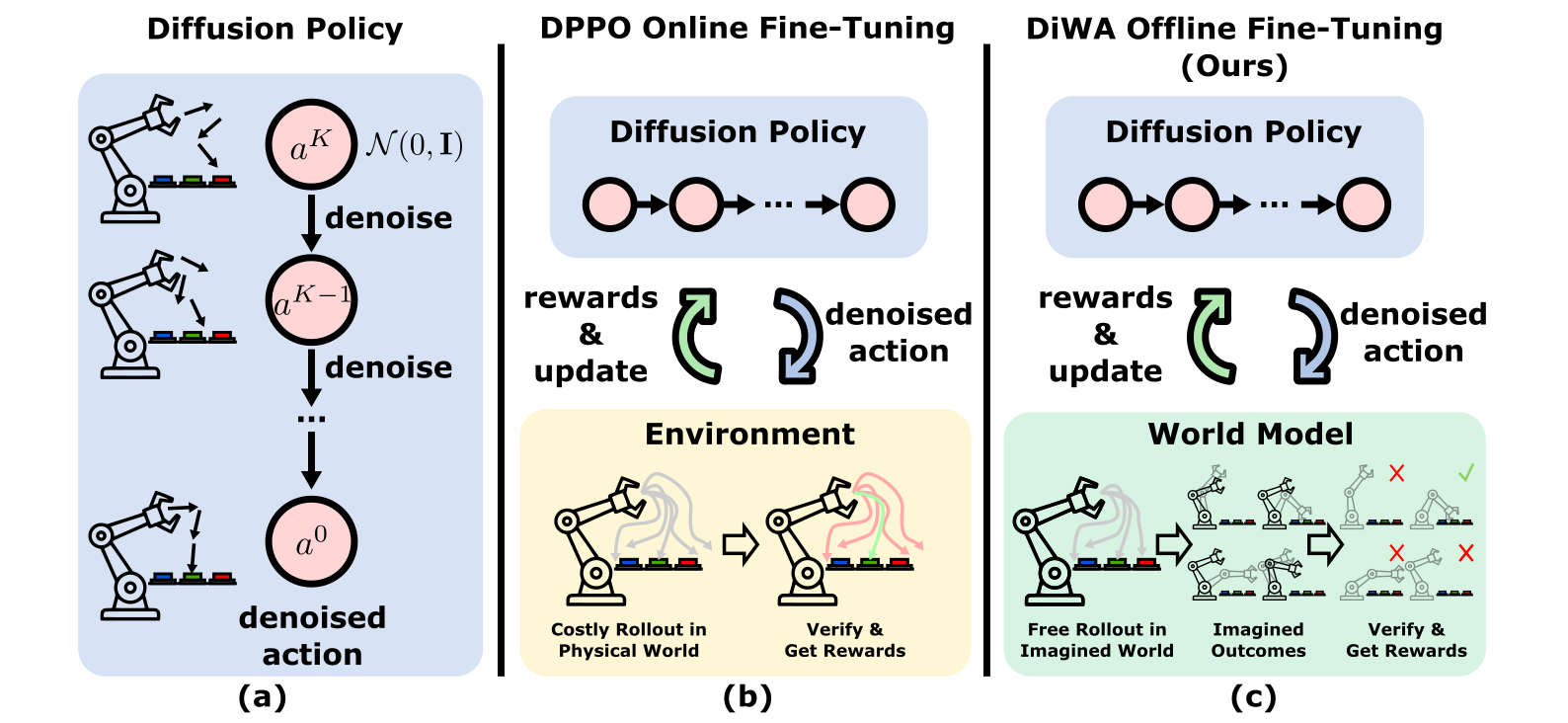
Diffusion Policy captures multimodal actions but inherits demonstration coverage limits. DPPO applies policy gradients across denoising steps, at the cost of online environment rollouts. DiWA replaces those rollouts with a learned latent simulator. This shifts the bottleneck from repeated task-specific interaction toward world-model coverage, reward accuracy, and simulation exploitation; imagined rollouts are computational work, not cost-free data.
2 Related Work
The approach combines imitation initialization, reusable play-trained dynamics, and PPO-style diffusion adaptation. Unlike online model-based methods that continually refresh their dynamics, DiWA freezes its model before policy optimization. Its contribution is the integration of denoising-step optimization with offline imagination, rather than a guarantee that a frozen model predicts every improved policy’s behavior.
3 Problem Formulation
Two datasets are required: task-agnostic play for dynamics and a small task-specific expert set for policy and reward learning. Gaussian noise is progressively denoised into an action or action chunk. The desired objective is real-environment return, but optimization occurs in a latent Markov model with learned dynamics and rewards. Improvement in that surrogate therefore depends on its fidelity along the adapted policy’s trajectories.
Equations 1–2
| (1) |
| (2) |
4 Offline Adaptation of Diffusion Policy with DiWA
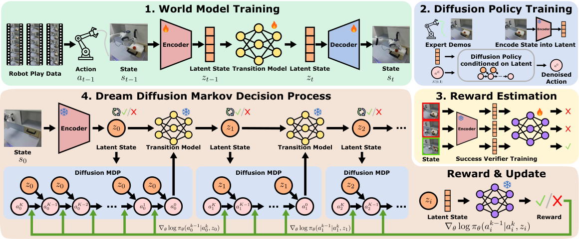
The four stages are world-model training, latent-conditioned behavior cloning, success-classifier training, and policy optimization in imagination. Dynamics, reward estimation, and the pretrained reference policy are fixed during adaptation. Deployment conditions the adapted policy on latents inferred from real observations.
4.1 World Model Learning
A recurrent state-space model combines a deterministic hidden state with categorical stochastic variables. An observation-conditioned posterior trains against a dynamics prior through reconstruction and KL terms, using straight-through gradients. During imagination, the prior advances without new images. Static and wrist-camera encoders follow the LUMOS design. Temporal state helps prediction but does not make long imagined trajectories ground truth.
Equations 3–4
| (3) | ||||||||
| (4) |
4.2 Pre-training Diffusion Policies
Fifty demonstrations per skill are encoded with the frozen world model. The diffusion policy learns demonstrated action sequences in that representation, aligning the interface used for imitation, imagination, and deployment. Separate policies are trained for each skill; this is not a single language-conditioned generalist policy.
4.3 Latent Reward Estimation from Expert Demonstrations
Annotated successful demonstration frames train a binary latent classifier. Its success probability supplies the reward during imagined action execution. Play is unlabeled, but the entire method is not reward-supervision-free. The main section evaluates the classifier on the next latent state, whereas the appendix writes a current-latent expression; both original conventions are retained and should be checked in implementation.
4.4 Dream Diffusion MDP
The Dream Diffusion MDP nests action denoising within world-model time. Intermediate denoising steps keep the same environment latent and receive zero reward. The final denoised action advances the latent dynamics, yields a classifier reward, and restarts from fresh Gaussian noise. Each Gaussian denoising transition has an explicit likelihood, enabling policy-gradient updates without needing the full marginal action-distribution likelihood.
Equations 5–8
| (5) |
| (6) |
| (7) |
| (8) |
4.5 Fine-tuning within Dream Diffusion MDP
PPO clips likelihood-ratio updates and discounts earlier, noisier denoising steps. A pretrained-policy regularizer is intended to reduce departures that exploit model errors. This restriction trades adaptation against fidelity to demonstrated behavior; it cannot certify correctness outside the model’s support. The published objectives and appendix algorithm are preserved rather than rewritten into a different regularizer.
Equations 9–11
| (9) |
| (10) |
| (11) |
5 Experimental Evaluation
Experiments separate simulated skill adaptation, latent-model/reward ablations, and physical execution of adapted policies. Online-baseline environment steps, offline play collection, imagined steps, and evaluation rollouts are different costs.
5.1 Simulation Results
CALVIN environment D supplies six hours of play, approximately five hundred thousand transitions, plus fifty demonstrations for each of eight skills. After five million imagined adaptation steps, drawer closing rises from 59.14% to 91.95%, lightbulb switching off from 35.63% to 77.01%, and LED switching on from 48.43% to 86.21%. Table 1 reports three-seed averages and deviations.
The matched latent-input DPPO baseline starts from the same policy and uses ground-truth rewards, while DiWA uses a learned classifier. Matching DiWA takes roughly 118,000–495,000 additional environment steps per skill for latent DPPO, and 134,000–2.25 million for pixel DPPO. These measurements are CALVIN simulator interactions despite the table’s “physical” label; DiWA’s zero excludes shared offline collection and evaluation. Pixel DPPO is faster than latent DPPO on the LED-off row, so the modality advantage is not uniform.
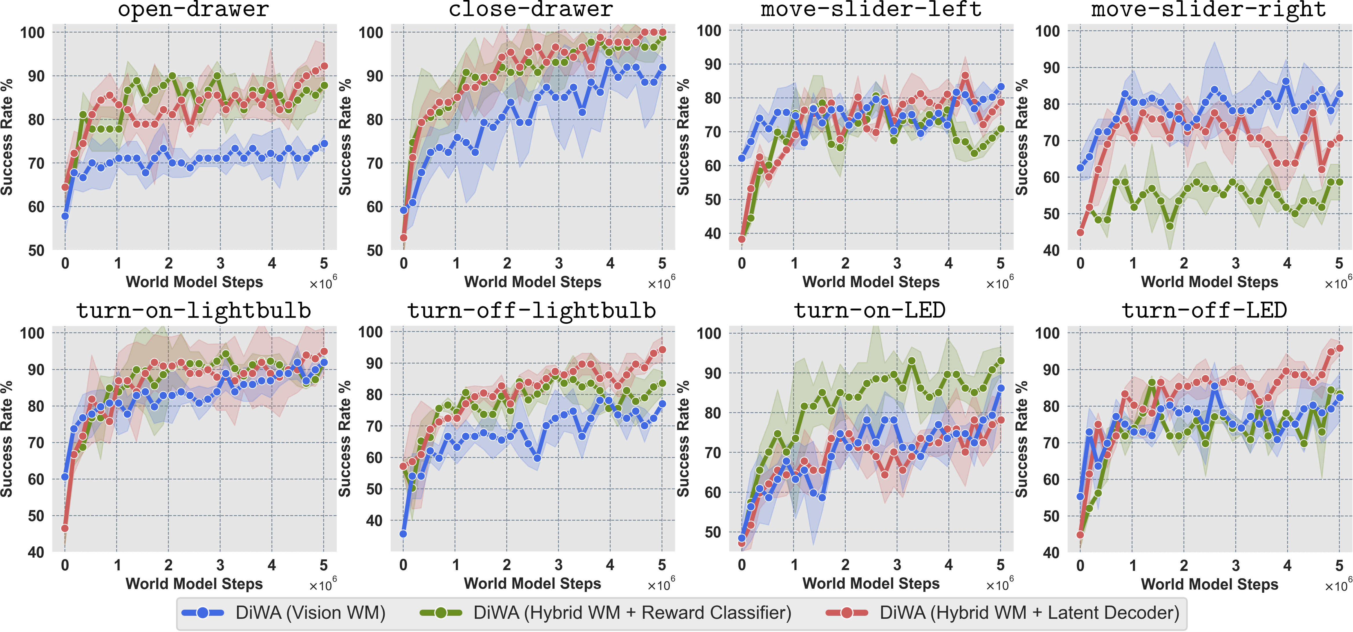
Hybrid models with privileged scene-state supervision adapt faster/more stably, and decoding state for reward can further improve results. These are diagnostic simulator variants; the main physical-compatible variant relies on vision. The comparisons support the importance of representation and reward quality without proving every gain comes from one component.
| Task | Base | DiWA (Ours) |
|
| ||||
| Diffusion Policy | Offline Fine-Tuning | Online Fine-Tuning | ||||||
| Success Rate | Success Rate | Env Steps to Match DiWA | ||||||
| open-drawer | ||||||||
| close-drawer | ||||||||
| move-slider-left | ||||||||
| move-slider-right | ||||||||
| turn-on-lightbulb | ||||||||
| turn-off-lightbulb | ||||||||
| turn-on-LED | ||||||||
| turn-off-LED | ||||||||
| Total Physical Interactions: | 0 | 2.5M | 8M | |||||
5.2 Real-World Results
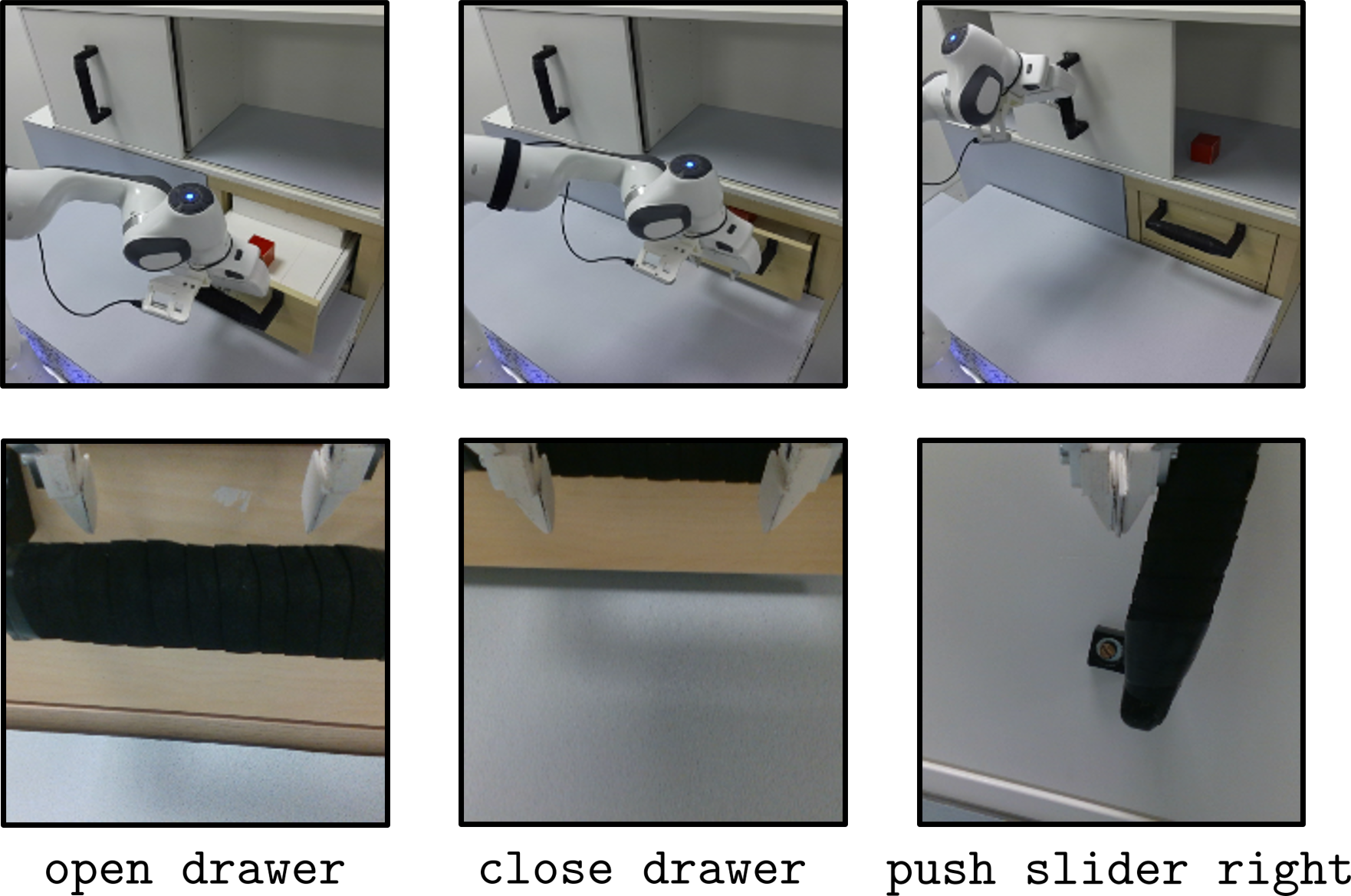
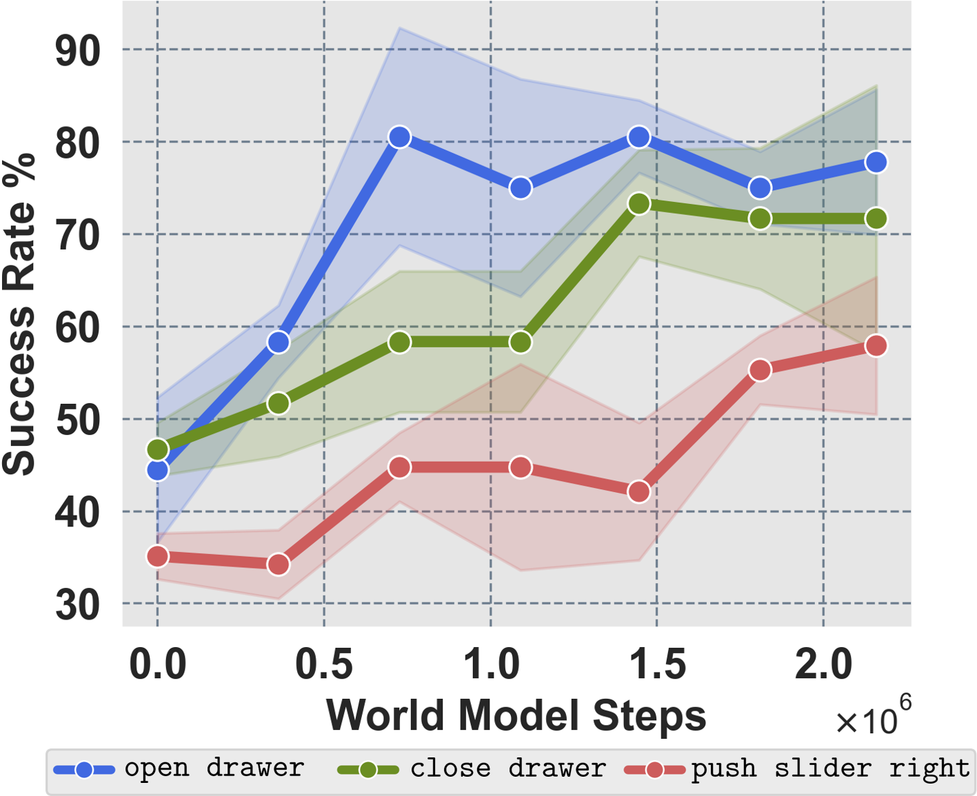
Four hours of physical Panda teleoperation, reported as about 450,000 recorded transitions, train the model; fifty extra expert demonstrations per skill initialize drawer opening, drawer closing, and slider-right pushing. Roughly two million imagined steps improve all three learning curves. Evaluation uses twenty rollouts per skill and three seeds with fixed initial configurations and robot poses. “No interaction” applies to gradient-update data collection, not those demonstrations or physical checkpoint evaluations. The study tests these three local skills rather than broad environment or object generalization.
6 Conclusion
A reusable offline world model can support diffusion-policy improvement with no new environment rollouts used for the adaptation updates. The physical results demonstrate imagination-to-robot transfer in a trained tabletop setting. Savings are best understood as avoiding additional task-specific online training interaction after collecting play and expert data.
7 Limitations
Frozen dynamics errors persist and may be exploited by the policy; high imagined reward can fail to transfer. The authors explicitly say intermediate checkpoints must be evaluated on the real system to assess true performance. This limits a strict interpretation of evaluation-free offline adaptation. Limited online model correction is proposed as future work, while adequate data coverage, reliable rewards, and checkpoint/regularization choices remain practical dependencies.
Acknowledgments
The authors acknowledge support from the University of Freiburg’s BrainWorlds initiative at the BrainLinks-BrainTools center.
Appendix S.1 Hyperparameters and Training Details
The supplementary settings specify the latent model, diffusion-policy training, reward classifier, and fine-tuning process. The complete original algorithm and every hyperparameter table are retained.
S.1.1 World Model
Two visual encoders feed a DreamerV2-style recurrent model. Thirty-two categorical variables with thirty-two classes form a 1,024-dimensional one-hot stochastic state; another 1,024 deterministic features give a 2,048-dimensional policy input. Training uses fifty-step sequences, batch fifty, recurrent reset probability 0.01, learning rate 3×10⁻⁴, and KL balancing 0.8. KL scale is 0.3 in simulation and 1.0 physically. Random subsequences stay within original episode boundaries.
| Name | Symbol | Value |
| Batch size | 50 | |
| Sequence length | 50 | |
| Deterministic latent state dimensions | — | 1024 |
| Discrete latent state dimensions | — | 32 |
| Discrete latent state classes | — | 32 |
| Latent dimensions | 2048 | |
| KL loss scale | 0.3 | |
| KL balancing coefficient | 0.8 | |
| RSSM reset probability | 0.01 | |
| World model learning rate | — | |
| Gradient clipping | — | 100 |
| Adam epsilon | ||
| Weight decay (decoupled) | — |
Equations 12–13
| (12) |
| (13) |
S.1.2 Diffusion Policy
The DDPM policy uses twenty denoising steps, one observation, and four predicted/executed actions per chunk. A three-layer 512-unit MLP trains for five thousand epochs on fifty demonstrations per skill, batch 256, with learning rate decaying from 10⁻⁴ to 10⁻⁵. EMA starts at epoch twenty. Baseline interfaces include 51-dimensional simulator state, two 64×64 RGB images stacked as six channels, or the same 2,048-dimensional world-model representation.
Equation 14
| (14) |
| Parameter | Symbol | Value |
| Common Training Parameters (All Skills) | ||
| Observation Horizon | — | 1 |
| Number of Demonstrations | 50 | |
| Planning Horizon | 4 | |
| Action Horizon | 4 | |
| Training Epochs | — | 5000 |
| Diffusion Denoising Steps | 20 | |
| Initial Learning Rate | — | |
| Final Learning Rate | — | |
| Weight Decay | — | |
| MLP Dimensions | — | [512, 512, 512] |
| EMA Decay | — | 0.995 |
| EMA Start Epoch | — | 20 |
| EMA Update Frequency | — | 10 |
| Batch Size | — | 256 |
| Observation Dimensions | ||
| DiWA | — | 2048 |
| DPPO (Vision WM Encoder) | — | 2048 |
| DPPO (Vision) | — | |
| DPPO (State) | — | 51 |
S.1.3 Latent Reward Estimator
Two 512/512 MLPs produce a contrastive embedding and success logits, trained with NT-Xent plus cross-entropy for one hundred epochs. Positives are annotated success frames; negatives sample fifteen percent of remaining frames. The retained validation table gives mean latent-classifier precision/recall 0.89/0.98 versus image ResNet-18’s 0.41/0.98. High recall alone does not prevent false-positive reward exploitation, and validation accuracy does not guarantee calibration on policy-generated imagined states.
Equations 15–16
| (15) |
| (16) |
| Parameter | Value |
|---|---|
| Embedding MLP | [512, 512] |
| Classification MLP | [512, 512] |
| Activation | ReLU |
| Output | Softmax |
| Epochs | 100 |
| Batch Size | 32 |
| Learning Rate | |
| Temperature | 0.5 |
| Loss | Contrastive+CE |
| Positives | Success frames |
| Negatives | 15% other frames |
| Task | Latents | Vision | ||
|---|---|---|---|---|
| Prec. | Rec. | Prec. | Rec. | |
| open-drawer | 0.92 | 0.99 | 0.41 | 0.99 |
| close-drawer | 0.89 | 0.99 | 0.52 | 0.99 |
| move-slider-left | 0.87 | 0.96 | 0.33 | 0.97 |
| move-slider-right | 0.83 | 0.98 | 0.41 | 0.99 |
| turn-on-lightbulb | 0.89 | 0.96 | 0.45 | 0.99 |
| turn-off-lightbulb | 0.88 | 0.99 | 0.36 | 1.00 |
| turn-on-LED | 0.94 | 1.00 | 0.36 | 0.92 |
| turn-off-LED | 0.88 | 0.99 | 0.41 | 0.99 |
| Avg. | 0.89 | 0.98 | 0.41 | 0.98 |
S.1.4 Fine-tuning with DiWA
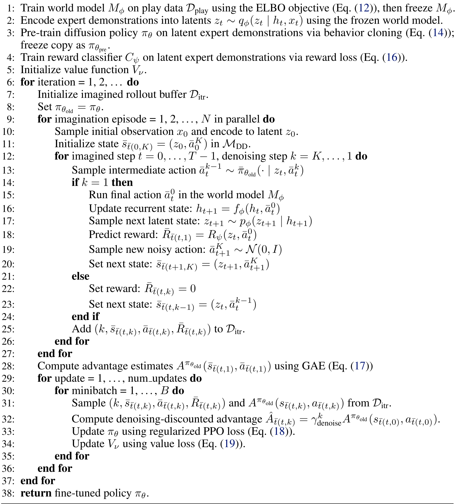
Algorithm S.1 preserves all thirty-eight lines, including nested imagination/update loops and their indentation. GAE is computed at action-completion steps, then denoising-discounted for policy updates. Only the last ten of twenty denoising steps are finetuned. Actor/critic learning rates are 10⁻⁵/10⁻³, world-model discount 0.999, diffusion discount 0.99, and GAE smoothing 0.95. Default cloning coefficient is 0.05, with task-specific 0.10/0.025/0.025 for opening/closing the drawer and turning on the LED. These selected coefficients are part of the experimental recipe, not a universally fixed setting.
Equations 17–19
| (17) |
| (18) |
| (19) |
| Parameter | Symbol | Value |
| Planning Horizon (Environment) | 4 | |
| Planning Horizon (Actor) | 4 | |
| Denoising Steps | 20 | |
| Fine-tuned Denoising Steps | 10 | |
| Actor Learning Rate | — | |
| Critic Learning Rate | — | |
| Actor MLP Dimensions | — | [512, 512, 512] |
| Critic MLP Dimensions | — | [256, 256, 256] |
| Discount Factor (Env /World Model) | / | 0.999 |
| Discount Factor (Diffusion Policy) | 0.99 | |
| GAE Smoothing Parameter | 0.95 | |
| Behavior Cloning Coefficient (default) | 0.05 | |
| Batch Size | — | 7500 |
Appendix S.2 Experimental Setup Details
Physical and simulation experiments share a seven-dimensional end-effector action interface. The physical observation/data pipeline is documented separately from the simulator’s privileged-state diagnostic variants.
S.2.1 7-DoF Action Framework
Actions contain three translation deltas, three Euler-angle deltas, and a gripper command, each normalized within ±1. The text says the environment uses +1 to close and −1 to open, but then says nonnegative policy outputs trigger opening and negative outputs closing. This apparent sign-convention mismatch is retained and flagged; deployment must verify the actual threshold mapping rather than copy a silently reconciled version.
Equation
S.2.2 Real-World Data Collection
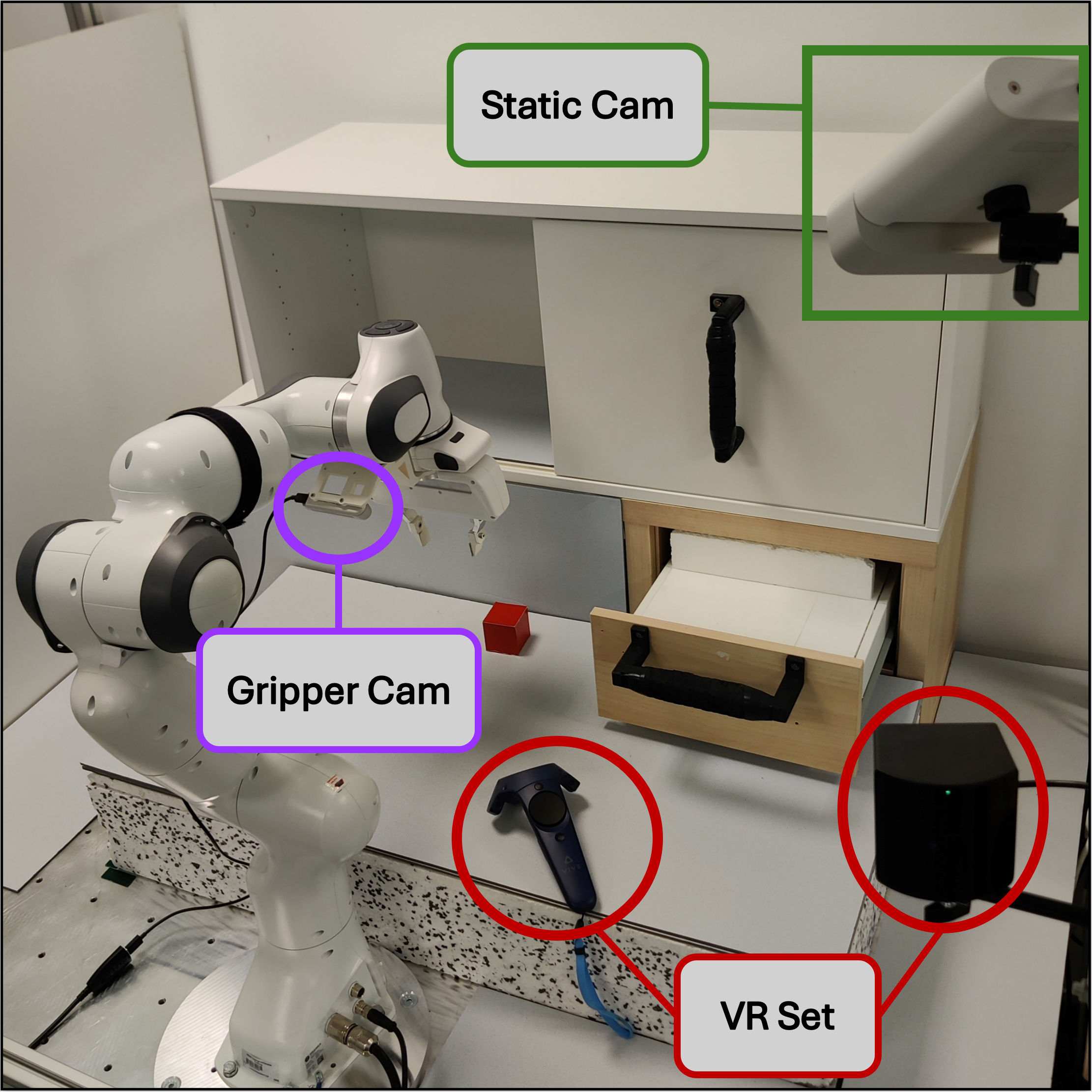
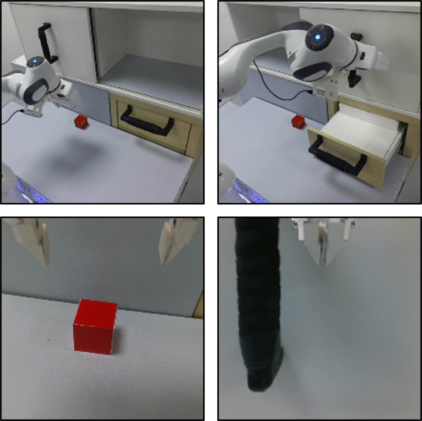
Panda teleoperation uses HTC VIVE with a tabletop cabinet/drawer and red cube. An Azure Kinect records static 200×200 views and a wrist RealSense D415 records close-ups, alongside robot state and absolute commands. Relative actions are consecutive command differences. Recording at thirty hertz is reduced to 7.5 hertz for training, so the approximately 450,000 transition headline should not be interpreted as a specified post-downsampling training count.
Appendix S.3 Data Preprocessing
Both cameras are resized to 64×64, converted to floating-point intensity, and normalized. Robot orientation preprocessing converts Euler angles to a continuous six-dimensional representation. These preprocessing details coexist with the paper’s vision-only main-model claim and privileged-state ablations; they do not imply every model receives the same state information.
Appendix S.4 Additional Experiments
Additional experiments examine online-input modalities, regularization, a Gaussian-policy variant, four LIBERO tasks, a failed offline-RL baseline, and qualitative physical-world predictions.
S.4.1 Comparing DPPO Input Modalities
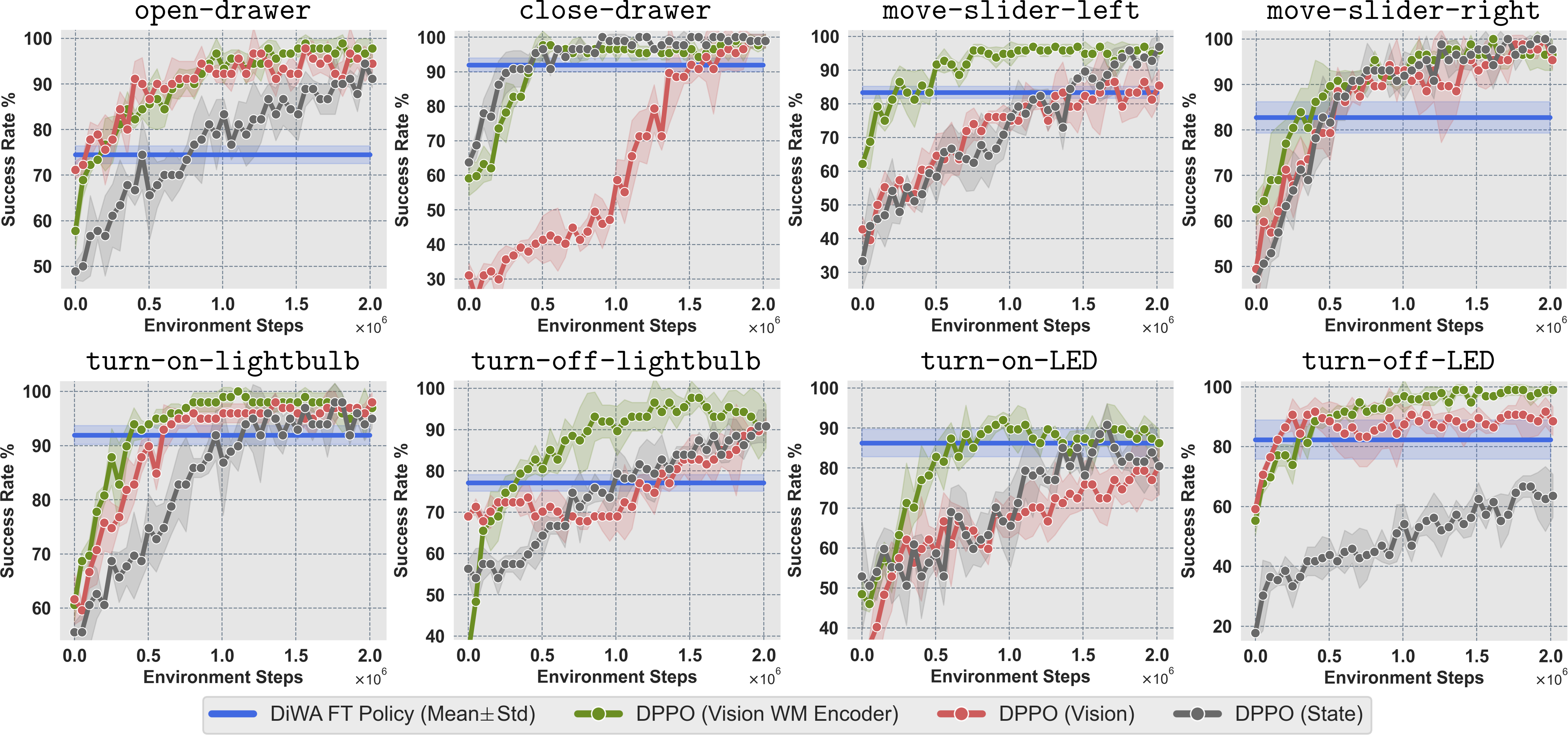
The frozen world-model representation often improves online DPPO over raw pixels or simulator-state inputs. Online variants can eventually match or exceed DiWA with additional ground-truth dynamics/reward interaction. DiWA’s horizontal band compares its offline-adapted result against that interaction axis; it does not imply no original data or no imagination computation. These are simulated baseline comparisons, not millions of measured hardware training steps.
S.4.2 Impact of Behavior Cloning Regularization
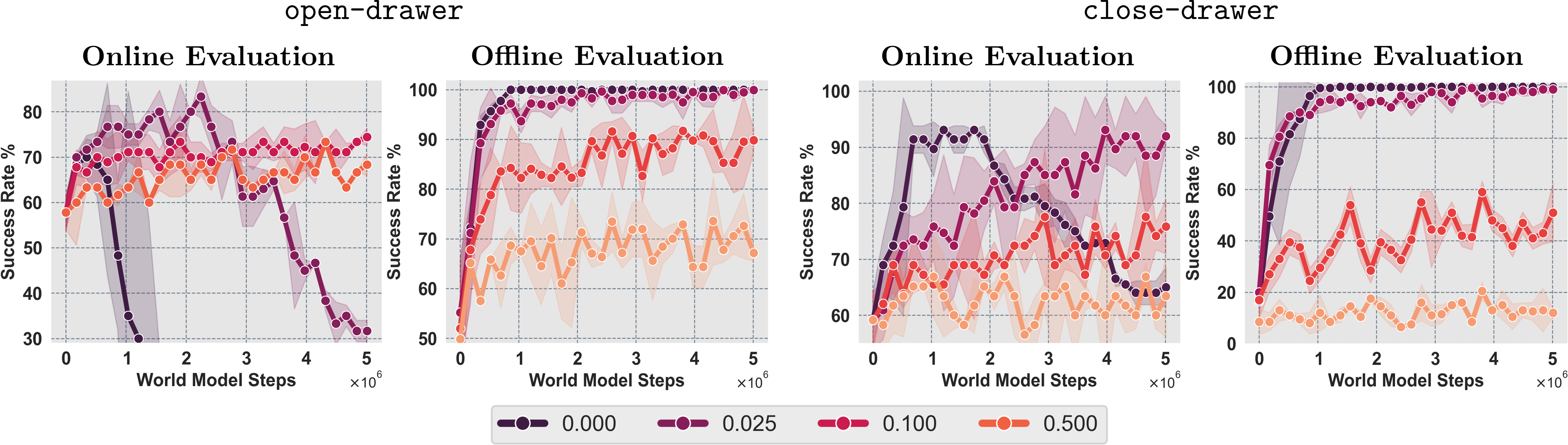
Without cloning regularization, imagined success rises while true-environment success deteriorates, consistent with model exploitation. A large coefficient such as 0.5 prevents useful adaptation; intermediate values perform better. Figure S.3 therefore demonstrates a substantive dependency on regularization and evaluation outside the model, not an automatic transfer guarantee. Future online model correction could reduce persistent errors.
S.4.3 Fine-tuning a Unimodal Gaussian Policy
Replacing diffusion with a diagonal-covariance Gaussian policy still improves all eight CALVIN tasks. Drawer closing rises from 55.17% to 98.28%, and slider-right from 55.52% to 87.93%. The benefit is therefore not exclusive to diffusion; imagination and reward learning can adapt a simpler policy too. The table is a separate policy-class experiment, not evidence that diffusion uniformly outperforms Gaussian policies.
| Task | Gaussian Policy | |
|---|---|---|
| Pre-Trained | Offline Fine-Tuned | |
| open-drawer | ||
| close-drawer | ||
| move-slider-left | ||
| move-slider-right | ||
| turn-on-lightbulb | ||
| turn-off-lightbulb | ||
| turn-on-LED | ||
| turn-off-LED | ||
| Total Physical Interactions: | 0 | |
S.4.4 Results on LIBERO-90
A model trained on LIBERO-90 demonstrations is evaluated on four kitchen skills across four scenes. Three-seed mean success improves from 40.67% to 77.33% for opening a top drawer, 54% to 91.33% for turning on a stove, 27.33% to 78% for closing a bottom drawer, and 75.33% to 100% for closing a top drawer. Imagined horizons are task-selected at three, two, one, and three million steps to avoid exploitation. This supports transfer across selected scene/task cases, not evaluation of all ninety tasks.
S.4.5 Offline RL Limitations in Our Setting
The attempted CQL baseline used play relabeled by the lower-precision image reward classifier and heuristic pseudo-episodes, then diverged. Reward noise, coverage, and value extrapolation are offered as explanations. This does not establish that all critic-based offline RL is inherently incompatible: the reward representation differs from DiWA’s stronger latent classifier, and no matched successful baseline is reported. DiWA itself also trains a value critic and remains vulnerable to model/reward error.
S.4.6 World Model Rollouts in the Real World
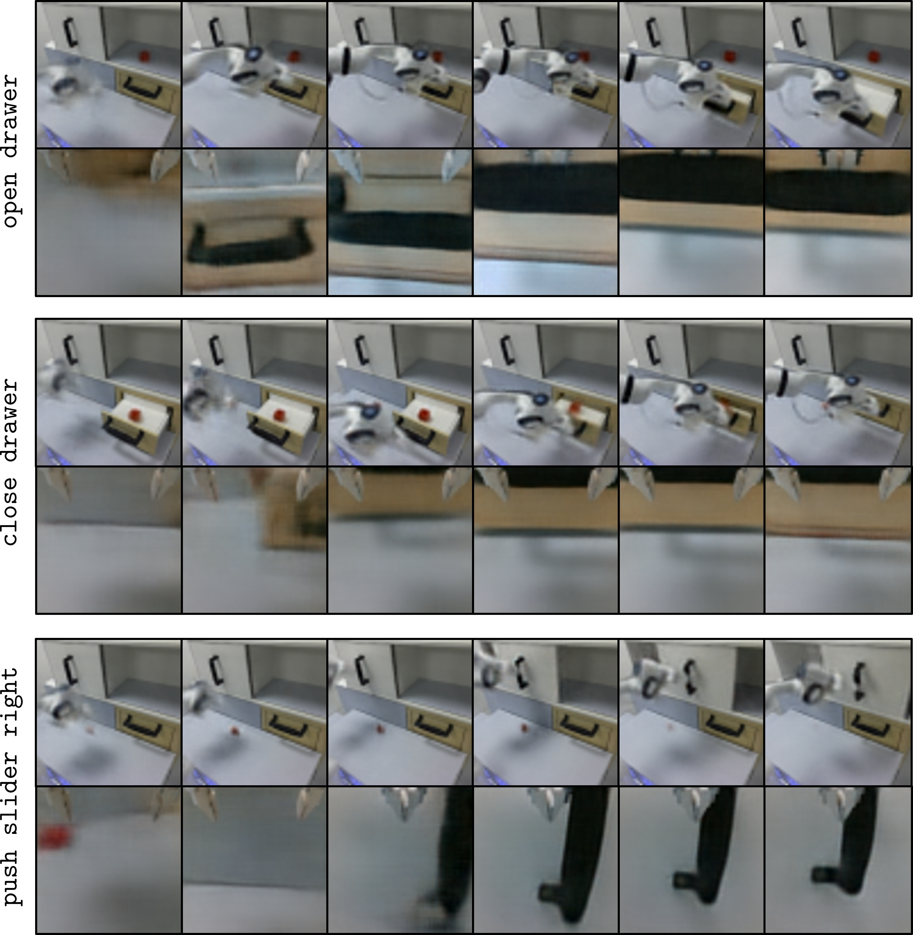
Two held-out frames initialize the model, which predicts eighty latent steps despite training on fifty-step sequences. Decoded static/wrist views qualitatively preserve robot and object structure. These examples illustrate temporal coherence; no quantitative eighty-step dynamics-error bound or guarantee of contact/control fidelity is supplied.