Overview
This edition follows the 35-page ICLR 2026 paper, arXiv version 3 dated 20 April 2026. It retains the complete method, experiments, tool interfaces, prompts, qualitative examples, and failure analysis. The central evidence concerns offline behavioral prediction and open-loop trajectory evaluation.
At a glance
DriveAgent-R1 is a 3B-parameter driving model that chooses between reasoning from its initial image and using visual tools for additional evidence. Domain alignment, dual-mode supervised training, and two reinforcement-learning stages teach tool execution and mode selection. It improves the reported offline planning scores with lower latency than supplying all camera views, but those comparisons do not establish human-level driving safety or closed-loop reliability.
1 Introduction
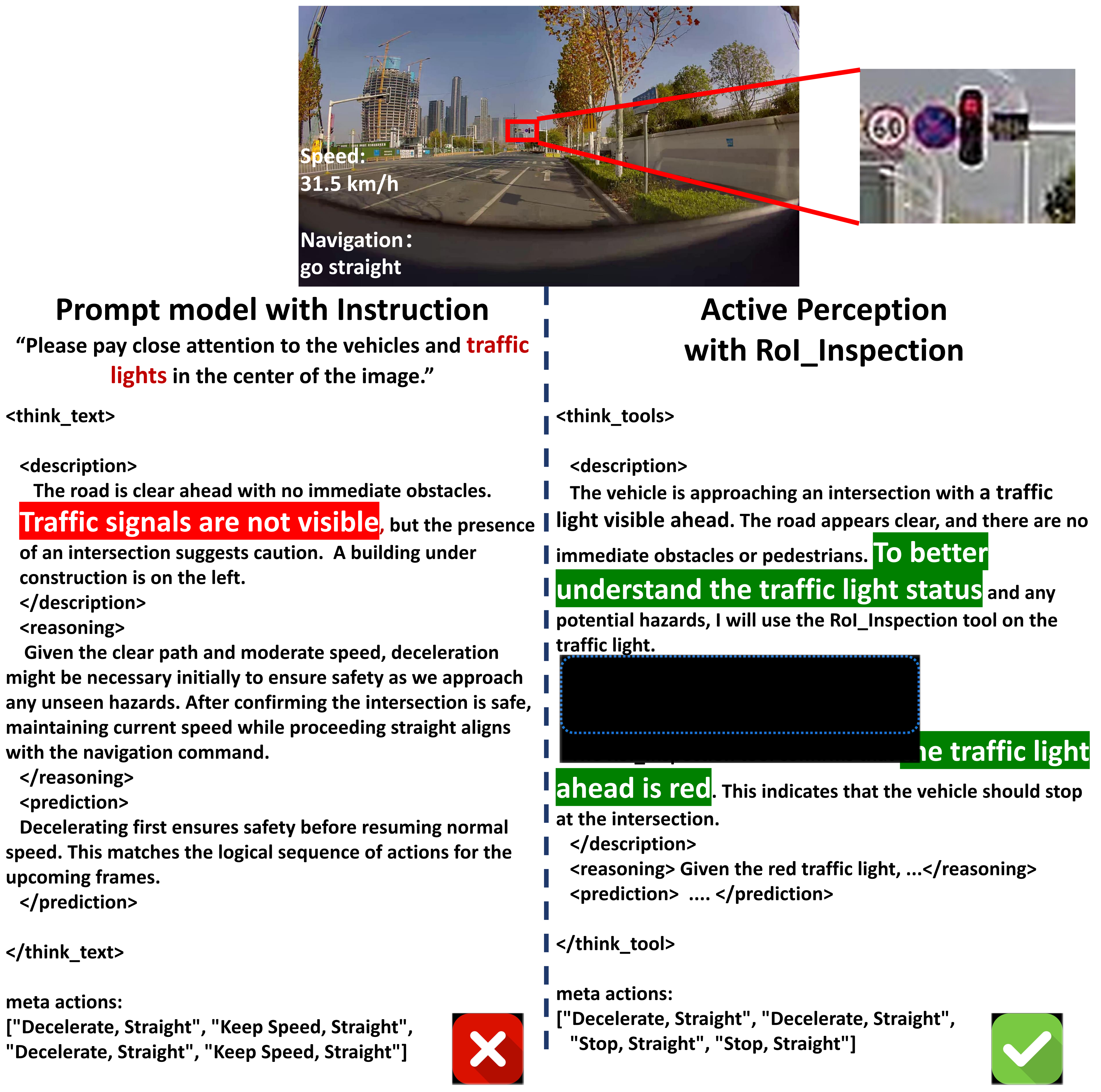
A fixed camera view may hide a distant signal or hazard, while always processing every view adds irrelevant information and cost. The proposed response is selective perception: decide whether extra evidence is needed, then request a camera view, crop, depth map, or object detector. This extends VLM driving approaches such as DriveVLM toward adaptive information acquisition. Here “text mode” still receives the initial image; it means reasoning without subsequent visual tool calls.
2 DriveAgent-R1
The system predicts coarse driving intentions, aligns its base model to driving scenes, and progressively learns both reasoning modes before learning when to choose each one.
2.1 Problem Formulation and Hybrid Thinking
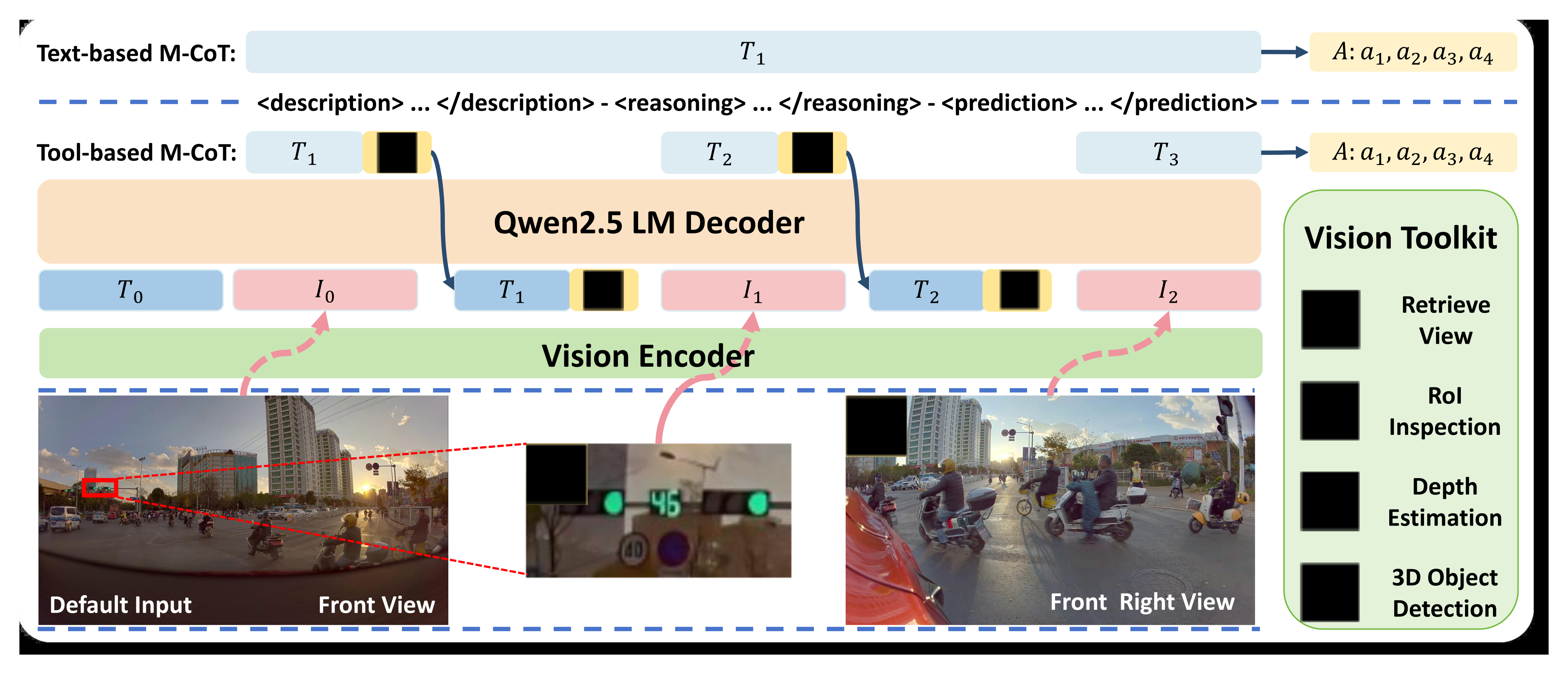
From the front camera, speed, and navigation instruction, the model predicts four speed–direction pairs at two-second intervals, described as an eight-second horizon. Speed choices are accelerate, maintain, decelerate, and stop; direction choices are straight, left, and right. Text mode reasons from the initial context. Tool mode interleaves scene description, reasoning, and prediction with new visual evidence until it outputs actions or reaches the interaction limit. The toolkit provides view/history retrieval, high-resolution region inspection, monocular depth, and open-vocabulary 3D detection.
Equation
2.2 Autonomous Driving Domain Alignment
All parameters of Qwen2.5-VL-3B are first fine-tuned on 530K driving visual question–answer pairs spanning scene description, traffic-entity recognition, target localization, and rules. The resulting DriveAlign-3B initializes every later stage. The motivation, also raised in Drive-R1, is to reduce reliance on speed/navigation shortcuts when images contain crucial evidence.
2.3 Progressive Training via SFT and Cascaded RL
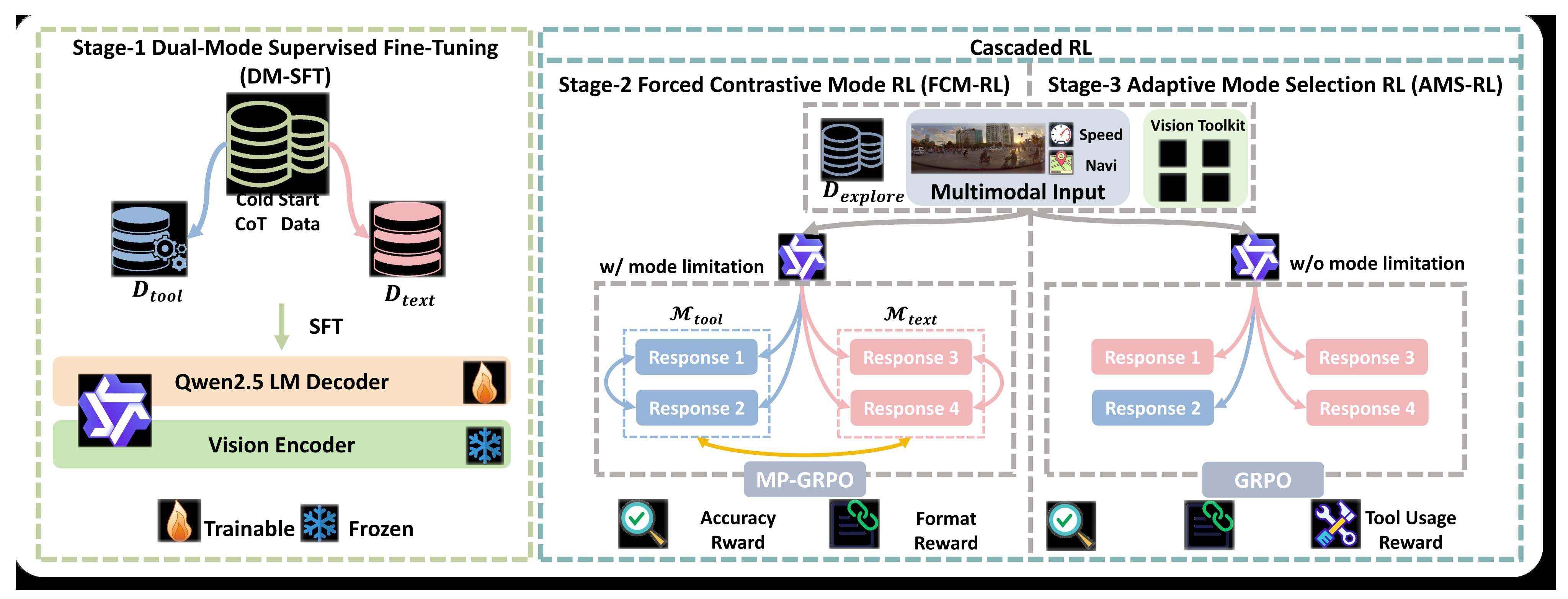
The three stages establish a common output format, strengthen both forced modes, then optimize adaptive mode selection. Figure 3 distinguishes this planning training from the earlier all-parameter domain alignment: its vision encoder is frozen during the depicted stages.
2.3.1 Stage 1: Dual-Mode Supervised Fine-Tuning
The supervised cold start uses balanced tool-needed and tool-unneeded examples. A small model identifies easy no-tool cases; a 72B teacher identifies cases improved by tools, generates mode-specific reasoning conditioned on known actions, and regenerates examples rejected by a judge. Rule-based cleaning checks format, final actions, and tool usage. This teaches a reasoning format from synthetic, label-conditioned demonstrations.
2.3.2 Stage 2: Forced Contrastive Mode Reinforcement Learning
Mode-partitioned GRPO extends the group-relative optimization used by DeepSeek-R1. Each query forces half its sampled responses into each mode, then normalizes rewards over the combined group. Thus weaker modes remain explored while responses compete both within and across modes. Rewards combine weighted action-sequence similarity and format consistency; incorrect mode/tool structure is penalized. This is distinct from normalizing each mode independently.
Equations
2.3.3 Stage 3: Adaptive Mode Selection Reinforcement Learning
The final GRPO stage lets the policy generate its own mode token. Tool responses receive an additional reward based on improvement over the group’s average no-tool response, minus a per-call cost. This encourages evidence that changes action quality rather than tool use for its own sake. If no text-mode response occurs in the group, the appendix sets this additional reward to zero.
Equation
3 Experiments
Experiments evaluate offline intention prediction, DriveBench, an added motion head, ablations, and latency. The comparisons use discrete labels inferred from recorded trajectories; they do not run an autonomous vehicle in a closed feedback loop.
3.1 Setup
The setup separates an internal long-tail training/test source from a public cross-dataset test, uses relaxed joint-action scores, and measures whether adaptive selection matches the better forced mode.
3.1.1 Dataset
Drive-Internal supplies the planning training data and the in-distribution test. nuScenes supplies a separately evaluated intention-prediction test; the motion-head extension later trains on nuScenes as a different experiment.
Automated Label Generation for Meta-actions.
Kinematic rules convert three-second trajectory windows into four meta-actions. Thresholds are adjusted using VLM consistency judgments and human spot-checks; GPT-4.1 then refines difficult cases from bird’s-eye trajectory visualizations. These are recorded-behavior labels, not independently established optimal actions for every scene.
Training Data.
Drive-Internal contains 35K clips across more than 40 complex or rare situations. One or two event-focused frames per clip are sampled. Supervised training uses 4K reasoning examples, equally divided by mode; cascaded RL uses a distinct 15K-instance exploratory set with balanced action distributions across sequence positions.
Test Data.
Evaluation uses 1,500 internal instances and 2,000 middle-of-clip nuScenes validation instances. The same trajectory-to-action labeling pipeline is applied to both sources. The paper describes random instance sampling; it does not provide a detailed clip-level leakage audit or geographic split analysis.
3.1.2 Evaluation Metrics
First-frame and sequence-average joint scores require matching speed and direction, but conservative speed errors can receive partial credit of 0.5 or 0.2. Sequence accuracy therefore means an average over the four steps, not exact correctness of the entire sequence. Mode-selection accuracy compares the selected mode with whichever forced mode scores better on that sample; tie handling and repeated-sampling uncertainty are not detailed.
Equation
3.1.3 Implementation Details
Training uses eight H20 GPUs and caps each image at 259,200 pixels. The default input is front-view only. RL samples four responses per query at temperature 1.0 and permits at most three tool calls; evaluation uses temperature 0.7. The reported stochastic evaluations should be read as this particular configuration.
| Model | Drive-Internal | nuScenes | ||||||
| First-Frame Joint Acc. (%) | Seq. Avg. Joint Acc. (%) | First-Frame Joint Acc. (%) | Seq. Avg. Joint Acc. (%) | |||||
| w/o Tools | w/ Tools | w/o Tools | w/ Tools | w/o Tools | w/ Tools | w/o Tools | w/ Tools | |
| Human | 49.59 | 49.29 | 50.48 | 48.24 | ||||
| Qwen2.5-VL-3B | 24.06 | 23.64 (-0.42) | 24.98 | 22.63 (-2.35) | 30.18 | 28.17 (-2.01) | 23.48 | 21.58 (-1.90) |
| Qwen2.5-VL-7B | 27.58 | 24.01 (-3.57) | 29.84 | 24.98 (-4.86) | 33.11 | 32.84 (-0.27) | 27.60 | 28.82 (+1.22) |
| Qwen2.5-VL-72B | 32.76 | 32.97 (+0.21) | 38.80 | 39.61 (+0.81) | 43.26 | 43.87 (+0.61) | 39.13 | 40.47 (+1.34) |
| Doubao-Seed-1.6 | 34.92 | 38.98 (+4.06) | 40.22 | 41.37 (+1.15) | 45.63 | 46.29 (+0.66) | 41.91 | 43.10 (+1.19) |
| Gemini-2.5-Flash | 41.83 | 43.38 (+1.55) | 42.14 | 43.42 (+1.28) | 45.46 | 46.60 (+1.14) | 42.69 | 44.07 (+1.38) |
| GPT-4.1 | 39.99 | 43.18 (+3.19) | 42.14 | 43.43 (+1.29) | 46.84 | 48.25 (+1.41) | 43.63 | 44.72 (+1.09) |
| GPT-5 | 56.30 | 56.48 (+0.18) | 47.19 | 47.97 (+0.78) | 48.75 | 49.11 (+0.36) | 44.85 | 45.14 (+0.29) |
| DriveAgent-R1 | 45.27 | 51.34 (+6.07) | 43.29 | 45.42 (+2.13) | 52.58 | 52.96 (+0.38) | 44.43 | 47.10 (+2.67) |
3.2 Main results
Main comparisons cover general VLMs, three human annotators, and specialized driving models. Toolkit access can help or hurt depending on model capability and training.
3.2.1 Comparison with SOTA VLMs and Human Drivers
With toolkit access, DriveAgent-R1 scores 51.34/45.42 on internal first-frame/sequence metrics and 52.96/47.10 on nuScenes. Its nuScenes sequence score exceeds GPT-5’s 45.14, but its internal sequence score is below GPT-5’s 47.97 and the human 49.29; human nuScenes sequence accuracy is 48.24. Tool access adds 6.07 internal first-frame points but only 2.13 sequence points. Smaller unadapted Qwen models often worsen with tools. Closed models use official APIs in the paper’s “no-thinking” setting with one-shot structured prompting, so this is a configured benchmark comparison.
3.2.2 Performence on DriveBench
On DriveBench, DriveAgent-R1 leads the three compared models in perception (34.07) and behavior (43.69). It does not lead every task: DriveLM has higher prediction (44.33 versus 32.85) and planning (68.71 versus 61.89). These task scores support better performance in some scene-understanding and decision categories, not an unqualified advantage across driving capabilities.
3.3 Performence of Motion Planing
A lightweight MLP consumes frozen-model visual tokens, one-hot meta-actions, and ego status to predict three-second waypoints at 2 Hz. On nuScenes, average displacement error is 0.28 m, versus 0.31 m for DriveVLM-Dual. Average collision rate is 0.14%, versus 0.10% for DriveVLM-Dual and 0.12% for UniAD. The extension is open-loop, and the presented comparison does not separately ablate meta-actions to establish that they alone cause the gain.
| Model | ADE (m) | Collision Rate (%) | ||||||
| 1s | 2s | 3s | avg | 1s | 2s | 3s | avg | |
| UniAD | 0.44 | 0.67 | 0.96 | 0.69 | 0.04 | 0.08 | 0.23 | 0.12 |
| VAD-Base | 0.17 | 0.34 | 0.60 | 0.37 | 0.07 | 0.10 | 0.24 | 0.14 |
| EMMA | 0.14 | 0.29 | 0.54 | 0.32 | - | - | - | - |
| DriveVLM-Dual | 0.15 | 0.29 | 0.48 | 0.31 | 0.05 | 0.08 | 0.17 | 0.1 |
| OmniDrive | 0.14 | 0.29 | 0.55 | 0.33 | 0.00 | 0.13 | 0.78 | 0.3 |
| OpenDriveVLA (3B) | 0.14 | 0.30 | 0.55 | 0.33 | 0.02 | 0.07 | 0.22 | 0.1 |
| DriveAgent-R1 (Ours) | 0.13 | 0.24 | 0.47 | 0.28 | 0.01 | 0.12 | 0.30 | 0.14 |
| Model | DriveAlign-VQA | General Benchmarks |
| Qwen2.5-VL-3B | 72.9 | 64.4 |
| Qwen2.5-VL-7B | 77.0 | 68.9 |
| DriveAlign-3B | 84.6 (+11.7) | 66.4 (+2.0) |
| Base Model | Model | Seq. Avg. Joint Acc. (%) | |
| w/ image | w/o image (rel. drop) | ||
| Qwen2.5-VL-3B | DriveAgent-R1-Variant | 43.56 | 38.79 () |
| DriveAlign-3B | DriveAgent-R1 | 45.42 | 38.24 () |
3.4 Ablation on Domain Alignment
Domain alignment raises the driving VQA score from 72.9 to 84.6 and the aggregate general-benchmark score from 64.4 to 66.4. Downstream internal sequence score improves from 43.56 to 45.42. Removing images causes a larger relative decline after alignment, 15.8% versus 11.0%, consistent with increased visual reliance; this sensitivity is not proof that every visual inference is correct.
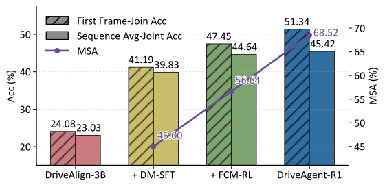
| Variant | Training Stage | Seq. Avg. Joint Acc. (%) | MSA (%) | ||||
| DM-SFT | FCM-RL | AMS-RL | |||||
| Variant-1 (SFT Only) | 1 epoch | - | - | 42.02 | 40.65 | 40.88 | 45.00 |
| Variant-2 (+FCM) | 1 epoch | 1 epoch | - | 44.30 | 42.20 | 44.64 | 56.64 |
| Variant-3 (+FCM x2) | 1 epoch | 2 epochs | - | 43.89 | 42.81 | 44.91 | 57.32 |
| Variant-4 (+AMS) | 1 epoch | - | 1 epoch | 43.78 | 41.64 | 43.43 | 57.55 |
| Variant-5 (+AMS x2) | 1 epoch | - | 2 epochs | 44.76 | 42.56 | 44.13 | 61.61 |
| DriveAgent-R1 (FCMAMS) | 1 epoch | 1 epoch | 1 epoch | 44.97 | 43.29 | 45.42 | 68.52 |
3.5 Ablation on Progressive Training Strategy
The complete cascade reaches 45.42 internal adaptive sequence accuracy and 68.52 mode-selection accuracy. It outperforms repeated single-stage alternatives with matched RL epoch counts. Forced-mode strengthening improves execution, while adaptive training improves selection; the combined schedule performs best in the reported table. Ablation differences are not accompanied by uncertainty intervals over training seeds. Figure 4 labels the supervised sequence score as 39.83, while Table 6 gives 40.88 for its adaptive SFT-only row; both original displays are retained.
| Model | Seq. Avg. Joint Acc. (%) | |
| w/ image | w/o image (rel. drop) | |
| Passive-FV | 42.70 | 39.64 (-7.2%) |
| Passive-SV | 43.10 | 39.01 (-9.5%) |
| DriveAgent-R1 (Retrieve View Only) | 44.39 | 38.78 (-12.6%) |
| DriveAgent-R1 (Full Toolkit) | 45.42 | 38.24 (-15.8%) |
3.6 Ablation on Active versus Passive Perception
Restricting the agent to view retrieval gives 44.39 internal sequence accuracy, above front-only passive input (42.70) and passive six-view input (43.10). The full toolkit reaches 45.42. Larger relative losses when images are removed indicate stronger dependence on vision. Selecting information from the same six-view pool helps here, but erroneous interpretation of selected evidence remains possible.
3.7 Efficiency Analysis
On one H20 GPU with batch size one and vLLM, adaptive inference averages 6.74 seconds and 265.57 output tokens, compared with 7.91 seconds/314.45 tokens in forced-tool mode and 8.50 seconds/210.77 tokens for passive surrounding views. Timings average 100 samples over five runs. Adaptive inference is about 20.7% faster than the passive baseline, but this seconds-scale benchmark is not evidence of meeting a real-time driving control deadline.
4 Related Work
Related work connects VLM scene understanding and planning, textual chain-of-thought, and tool-interleaved visual reasoning. The proposed distinction is the learned choice between initial-context reasoning and additional visual evidence, rather than a new low-level vehicle-control formulation.
5 Conclusion and Limitations
The results support adaptive tool use for the tested offline planning tasks. A documented failure shows that new evidence can override a correct initial judgment when the agent confuses road topology or signal ownership. The authors propose stronger traffic-rule alignment and conflict-aware reasoning. Closed-loop safety, robust real-time operation, and broad generalization beyond the evaluated data remain unestablished.
Acknowledgments
The work acknowledges sponsorship by the Beijing Nova Program.
Appendix A Appendix
The appendix provides exact tool interfaces and prompts, dataset generation, reward definitions, labeling rules, human-evaluation protocol, detailed ablations, successful examples, and a failure analysis.
A.1 Usage of LLM
The authors disclose using language models for manuscript polishing, grammar, and brainstorming component names; they attribute the methodology and experimental findings to the authors.
A.2 Vision Toolkit: Detailed Descriptions and Call Formats
The four retained call examples specify the serialized requests used for active perception. Their original code text and indentation are preserved.
Retrieve View.
View retrieval selects a camera and can access a five-second history sampled at 1 Hz. This lets the policy inspect another viewpoint or earlier observation without encoding every full video sequence. The example requests the front-left image one second earlier.
<tool_call>
    <tool_name>Retrieve View</tool_name>
    <params>{"frame_index": "-1s", "view_index": "front_left"}</params>
</tool_call>
RoI Inspection.
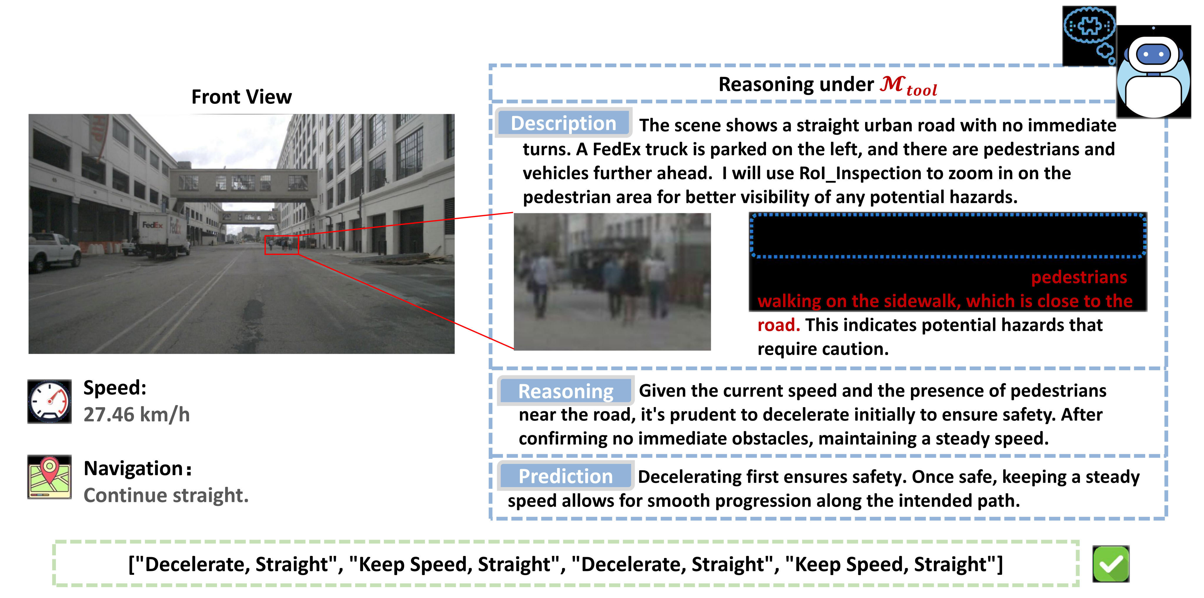
Region inspection uses absolute pixel bounding-box coordinates on a higher-resolution source image. Cropping and re-encoding adds visual detail that may be absent from compressed whole-image tokens; the agent must still localize the relevant region correctly.
<tool_call>
    <tool_name>RoI Inspection</tool_name>
    <params>{"view_index": "front_left", "bbox": [x_min, y_min, x_max, y_max], "description": "the traffic lights"}</params>
</tool_call>
Depth Estimation.
Depth maps come from Depth Anything V2. They offer monocular geometric cues for interpreting obstacles and scene layout, rather than independently verified metric measurements or safety guarantees.
<tool_call>
    <tool_name>Depth Estimation</tool_name>
    <params>{"view_index": "front"}</params>
</tool_call>
3D Object Detection.
The open-vocabulary monocular detector follows Detect Anything 3D and accepts a camera view plus an object description. It supplies location, size, and orientation cues for requested object classes; useful decisions still depend on correct detector outputs and interpretation.
<tool_call>
    <tool_name>3D Object Detection</tool_name>
    <params>{"view_index": "front", "object_text": "barrier"}</params>
</tool_call>
A.3 Dataset Construction
Two data pipelines serve different purposes: broad visual question answering establishes domain familiarity, while event-focused driving clips supply planning examples and action labels.
A.3.1 DriveAlign-VQA Dataset Construction
Starting from one million driving frames, CLIP clustering supports diverse image sampling. Qwen2.5-VL-72B generates questions using a 70% template/30% free-form mix, with either front-only or six-view images. Doubao-Seed-1.6 judges each pair, retains perfect-scoring examples, paraphrases questions, and filters trivial items. The result is 530K synthetic QA pairs; automated acceptance is not equivalent to comprehensive human verification.
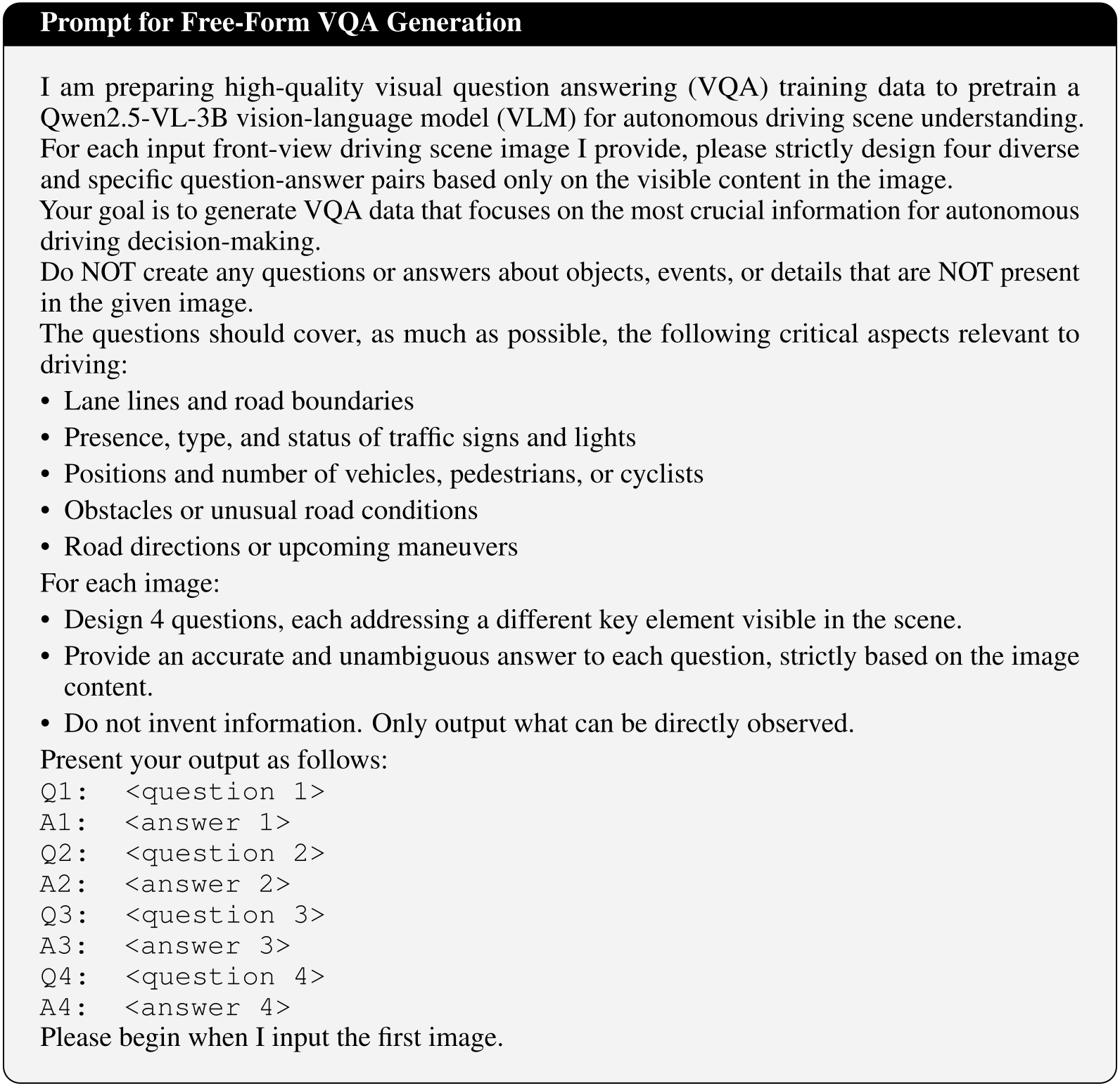
A.3.2 Construction Pipeline of Drive-Internal Dataset
CLIP retrieval and human inspection find unusual objects and corner cases; variability in driving maneuvers identifies difficult interactions. Keyframes for changing speed or direction precede the event by roughly 0.5–1.0 seconds, while steady scenes use an informative representative frame. This deliberately emphasizes decision-critical events rather than natural driving frequencies.
A.4 DM-SFT CoT Data Construction Pipeline
The supervised-reasoning pipeline separates easy and tool-benefiting cases, creates teacher reasoning from known action labels, and cleans the resulting demonstrations before equal sampling by mode.
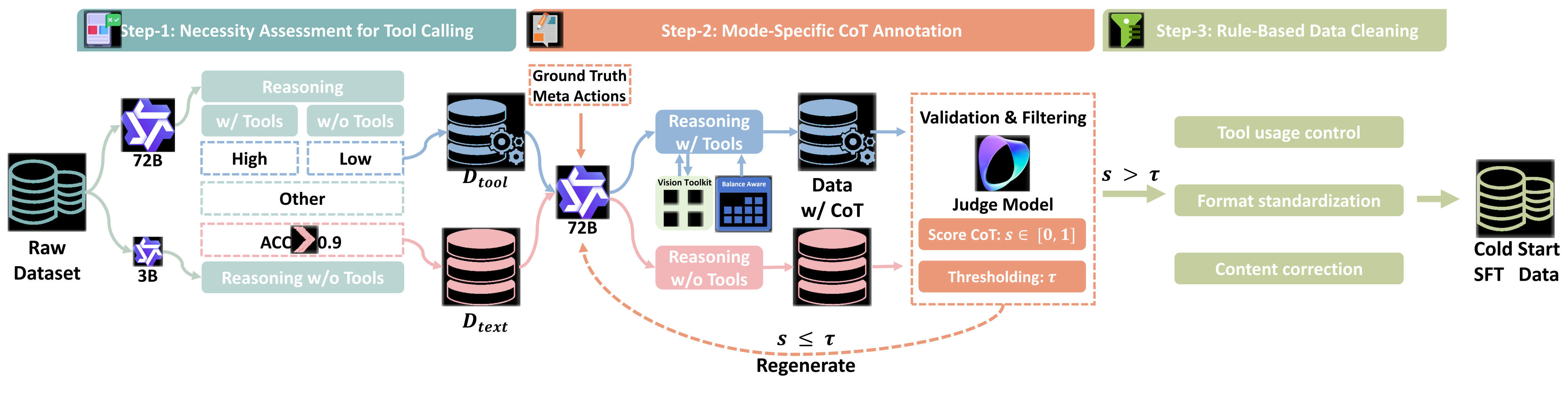
Step 1: Necessity Assessment for Tool Calling.
A small model’s high no-tool accuracy, with 0.9 given as an example threshold, identifies easy cases. The 72B oracle then identifies remaining examples that improve with tools; ambiguous cases are reserved for RL exploration. Thus “tool necessity” is operationally defined by these models’ performance, not a universal property of a scene.
Step 2: Mode-Specific CoT Annotation and Validation.
The teacher constructs reasoning backward from ground-truth meta-actions. A separate judge scores coherence and rejects low-scoring responses for regeneration; dynamic guidance balances tool preferences. These are synthetic rationales conditioned on the target answer, so their plausibility does not demonstrate faithful explanations of an independently reached decision.
Step 3: Rule-Based Data Cleaning.
Cleaning standardizes reasoning structure and call syntax, corrects artifacts or action-label mismatches, and limits redundant or illogical calls. Equal numbers from both mode categories form the 4K-example cold start.
A.5 Reward Design Details
Rewards combine position-weighted sequence similarity, output-format consistency, and conditional benefit from tools. The displayed formulas are retained because their weighting and missing-baseline behavior matter for interpreting the training objective.
Accuracy Reward ( R acc ).
Action reward weights speed similarity by 0.7 and direction similarity by 0.3. Each uses weighted Levenshtein distance normalized by sequence length, with insertion/deletion cost 0.6. Position-specific class weights derive from inverse frequencies with exponent 0.5, are clipped to a suggested 0.7–1.3 range, then normalized to mean one. Since exact-match weights can exceed one, this weighted reward is not simply a bounded raw accuracy probability.
Equations
Tool Usage Reward ( R tool ).
Tool reward subtracts the group’s mean no-tool accuracy and 0.125 per call from a tool trajectory’s accuracy, with an example clipping range of −0.2 to 0.2. If no no-tool trajectory is sampled, the term is zero. The cost is motivated by spreading a nominal 0.25 gain over two calls; that is a design heuristic, since actual accuracy reward is weighted and uses sequence alignment.
Equation
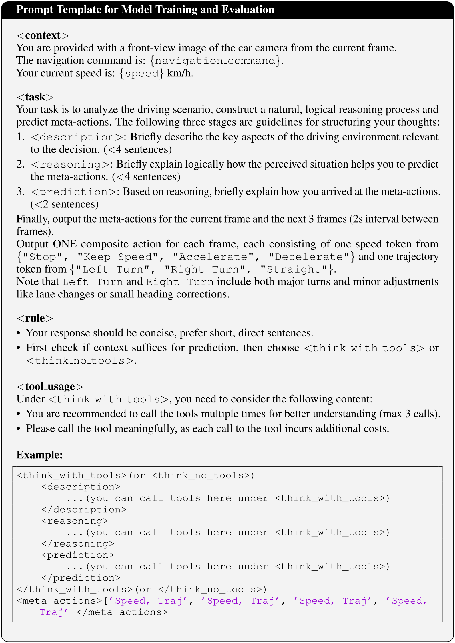
A.6 Training and Evaluation Prompt Template
The complete training/evaluation prompt constrains brief description, reasoning, prediction, four meta-actions, and at most three meaningful tool calls. It treats left/right actions as including small heading adjustments. Its example uses “think_with_tools” and “think_no_tools” tags, whereas the method text uses “think_tool” and “think_text”; the original template is retained without silently harmonizing this discrepancy.
A.7 Automated Meta-Action Labeling Pipeline
Recorded trajectories are discretized by kinematic rules, whose thresholds are iteratively adjusted against visual consistency judgments and human spot-checks. A final VLM pass refines ambiguous labels.
A.7.1 Rule-Based Generation
Rules operate on longitudinal motion and heading change within sliding windows, producing the speed–direction labels used for planning supervision and evaluation.
Sliding Window Mechanism.
Each three-second window includes one second of history and two seconds of future motion. Four windows advance in two-second increments from the current frame, producing the four-step behavioral sequence.
Trajectory-to-Action Mapping.
Speed below 0.5 m/s is labeled stop; acceleration magnitude beyond 0.3 m/s² distinguishes acceleration/deceleration from maintaining speed. Heading change below 15° is straight, otherwise its sign determines left or right. The authors report these as thresholds converged through feedback tuning; they are labeling conventions rather than universal vehicle-control thresholds.
A.7.2 Iterative Threshold Optimization and VLM-Based Refinement
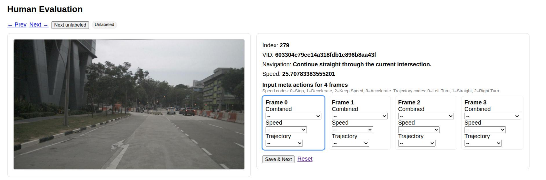
GPT-4.1 checks a bird’s-eye visualization against provisional labels while human spot-checks track errors. Thresholds are adjusted for agreement, then difficult residual examples receive final refinement. The preserved prompt restricts output to four legal action strings, disallows invented trajectory points, and handles stationary segments; detailed iteration histories and final label-error rates are not supplied.
A.8 Human Evaluation Details
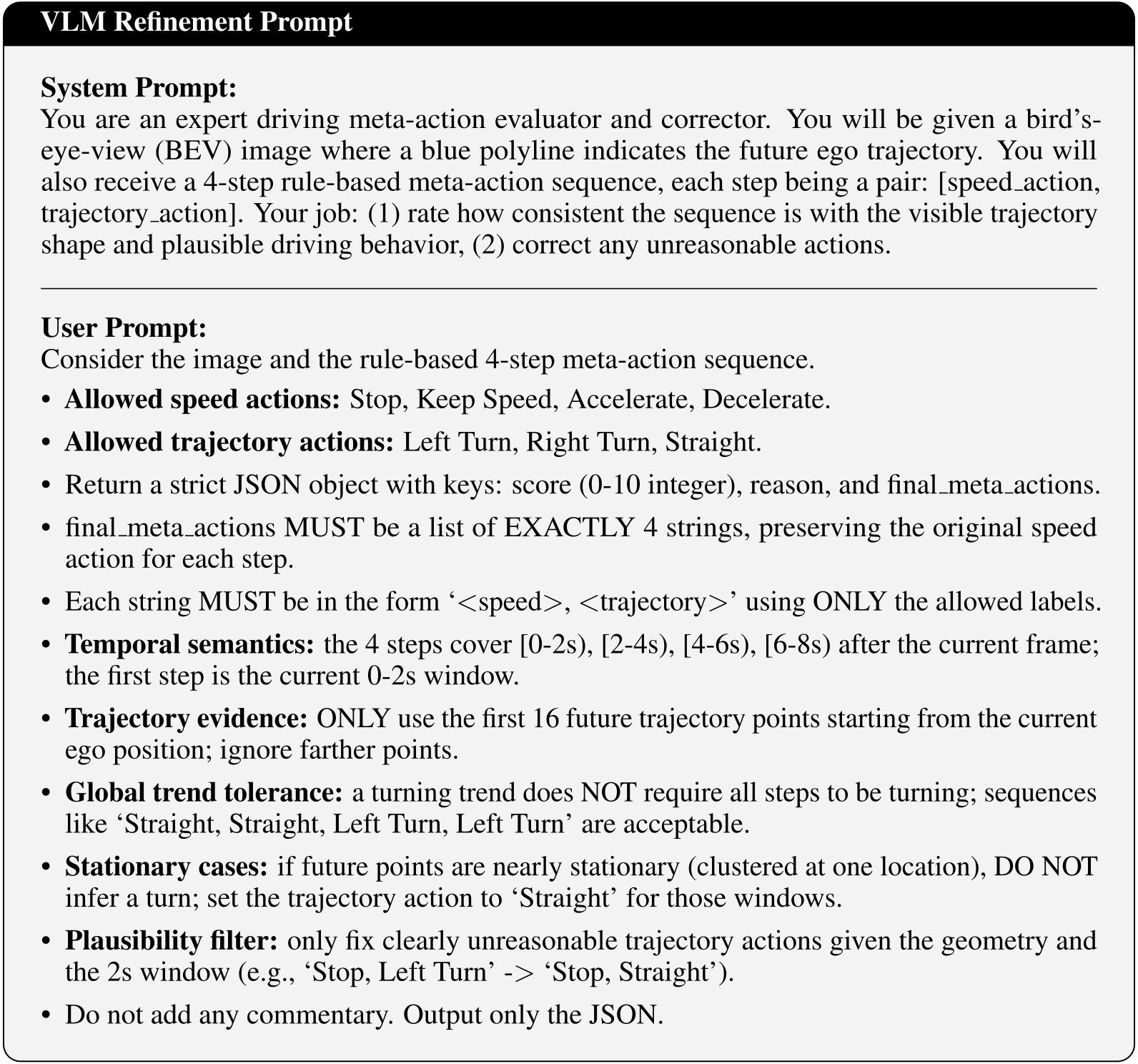
Three licensed drivers with over two years’ experience each label disjoint thirds of both test sets using front-view images, speed, and navigation. Their scores are averaged. They do not receive the agent’s interactive toolkit, and there is no repeated multi-rater labeling per item, so this measures the specified annotation task rather than real-world human driving proficiency.
A.9 Extended Experimental Results
Additional tables separate driving-VQA categories and general benchmarks, and repeat training ablations on nuScenes.
A.9.1 Detailed Results for Domain Alignment
The driving VQA test has 200 samples in each of four topics and uses Doubao-Seed-1.6 as judge. Alignment improves all four domain categories, with +11.7 aggregate points. General performance rises by two points on average, but individual results are mixed: MMVet and OCRBench decrease. Evaluation uses the listed VLMEvalKit defaults.
| Task | Benchmark | DriveAlign-3B (ours) | Qwen2.5-VL-3B | Qwen2.5-VL-7B |
| DriveAlign-VQA | scene description | 87.8 (+5.5) | 82.3 | 82.2 |
| recognition of traffic entities | 91.5 (+11.4) | 80.1 | 86.4 | |
| localization of critical targets | 85.1 (+12.9) | 72.2 | 67.9 | |
| traffic commonsense and rules | 74.0 (+17.1) | 56.9 | 71.5 | |
| overall | 84.6 (+11.7) | 72.9 | 77.0 | |
| General | MMStar | 56.7 (+2.9) | 53.8 | 60.6 |
| MMVet | 60.6 (-0.6) | 61.2 | 69.0 | |
| MMBench_EN (val) | 80.4 (+1.1) | 79.3 | 79.7 | |
| MMBench_EN_V11 (val) | 77.4 (+1.0) | 76.4 | 80.3 | |
| MME-Realworld-lite | 48.3 (+6.2) | 42.1 | 44.6 | |
| OCRBench | 81.4 (-1.2) | 82.6 | 88.1 | |
| MMMU (val) | 46.0 (+4.4) | 41.6 | 48.4 | |
| AI2D | 80.1 (+1.9) | 78.2 | 80.7 | |
| overall | 66.4(+2.0) | 64.4 | 68.9 |
Notes. For DriveAlign-VQA, each of the four topics contains 200 samples; the judge model is Doubao Seed 1.6. The general benchmarks suite includes MMStar (Chen et al., 2024), MMVet (Yu et al., 2024), MMBench (Liu et al., 2024a), MME-Realworld-lite (Zhang et al., 2024), OCRBench (Liu et al., 2024b), MMMU (Yue et al., 2024), and AI2D (Kembhavi et al., 2016). The general evaluation was performed using VLMEvalKit (Duan et al., 2024) with the default configuration.
A.9.2 Extended Ablation Results for Progressive Training Strategy
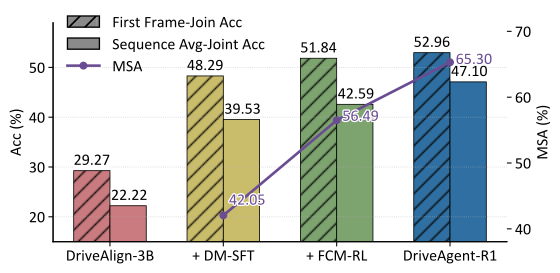
The complete cascade achieves 47.10 adaptive sequence accuracy and 65.30 mode-selection accuracy on nuScenes, compared with 39.53 and 42.05 after supervised training alone. Matched-epoch repeated-stage variants remain below the cascade in adaptive sequence score. These are cross-dataset intention results, distinct from the nuScenes-trained motion-head experiment.
| Variant | Training Stage | Sequence Avg-Joint Acc (%) | MSA (%) | ||||
| DM-SFT | FCM-RL | AMS-RL | |||||
| Variant-1 (SFT Only) | 1 epoch | - | - | 41.04 | 39.17 | 39.53 | 42.05 |
| Variant-2 (+FCM) | 1 epoch | 1 epoch | - | 42.92 | 40.58 | 42.59 | 56.49 |
| Variant-3 (+FCM x2) | 1 epoch | 2 epochs | - | 45.15 | 41.07 | 44.60 | 58.30 |
| Variant-4 (+AMS) | 1 epoch | - | 1 epoch | 41.18 | 40.58 | 40.92 | 57.76 |
| Variant-5 (+AMS x2) | 1 epoch | - | 2 epochs | 44.19 | 41.47 | 43.57 | 60.30 |
| DriveAgent-R1 (FCMAMS) | 1 epoch | 1 epoch | 1 epoch | 46.38 | 44.43 | 47.10 | 65.30 |
A.10 Qualitative Results
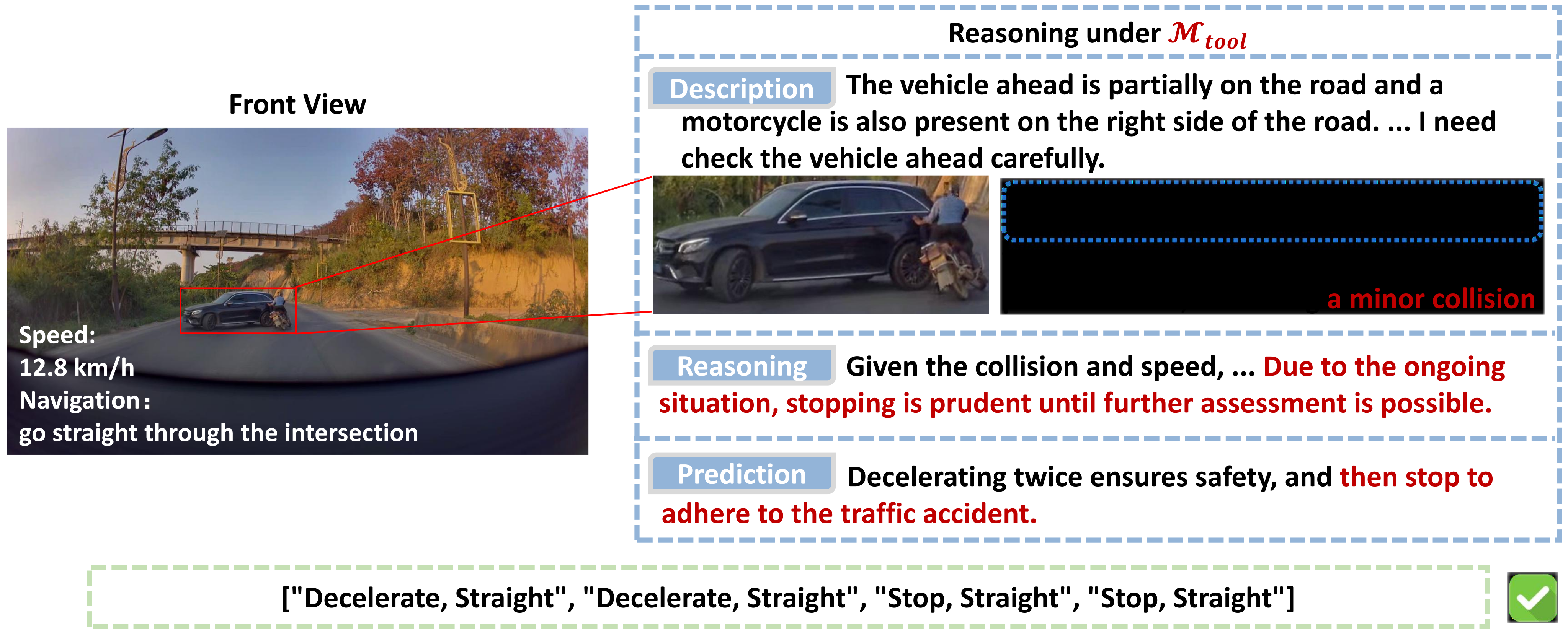
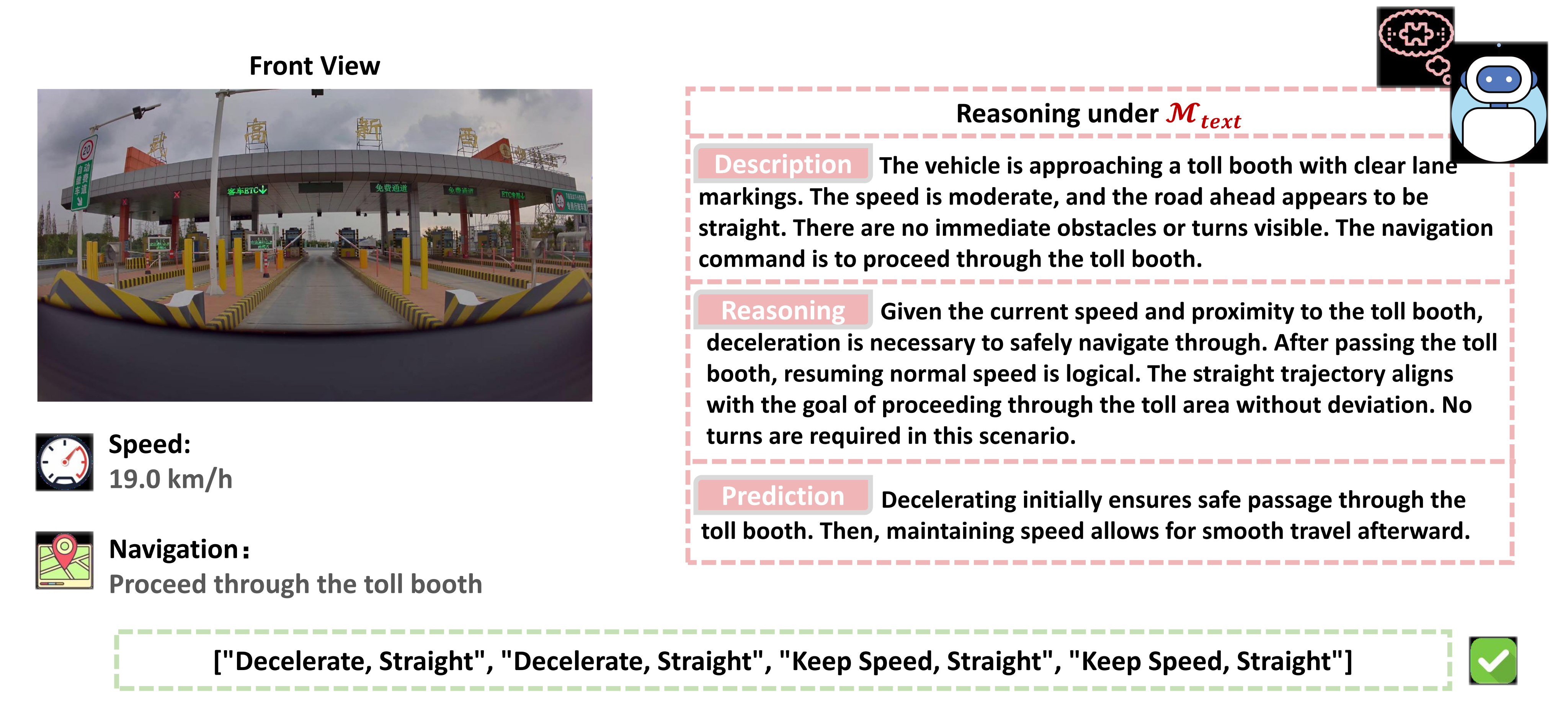
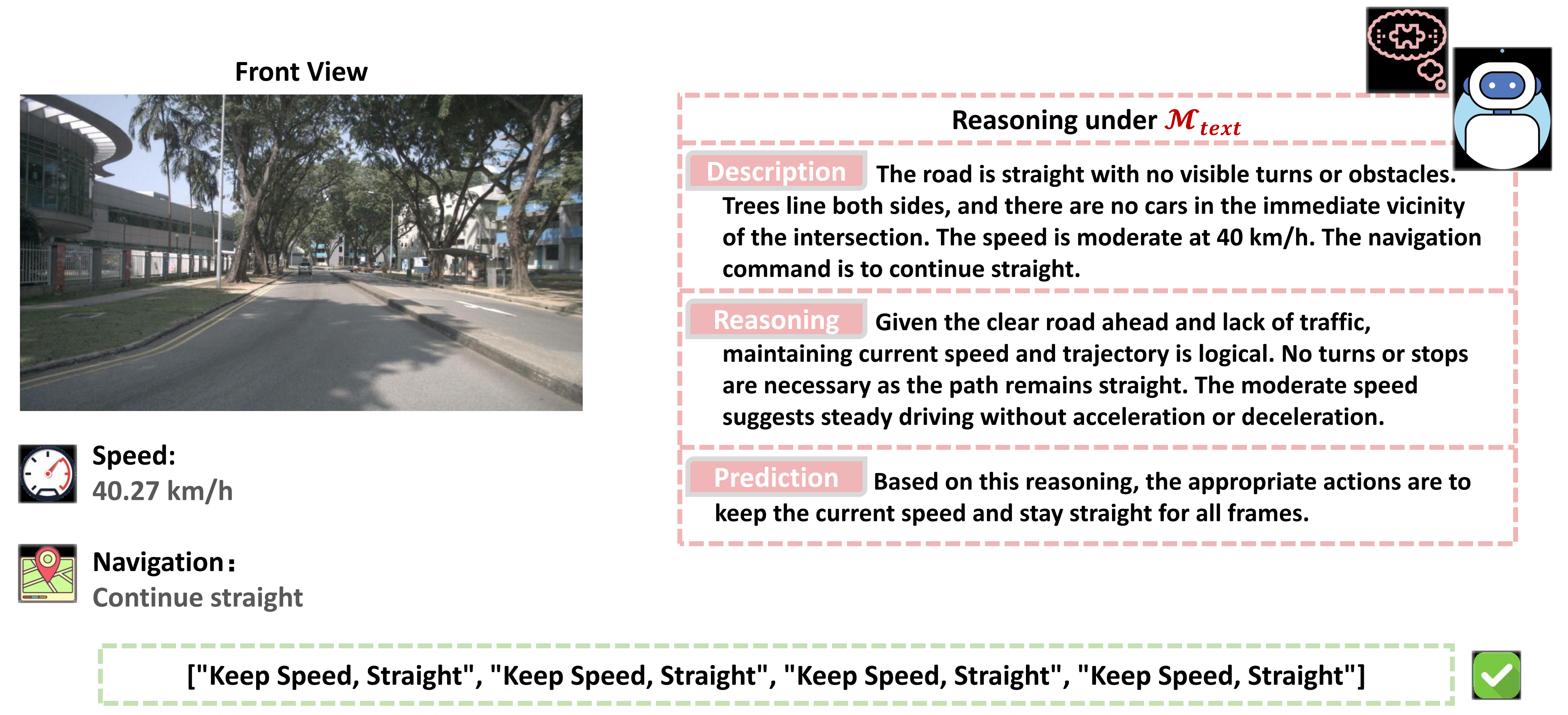
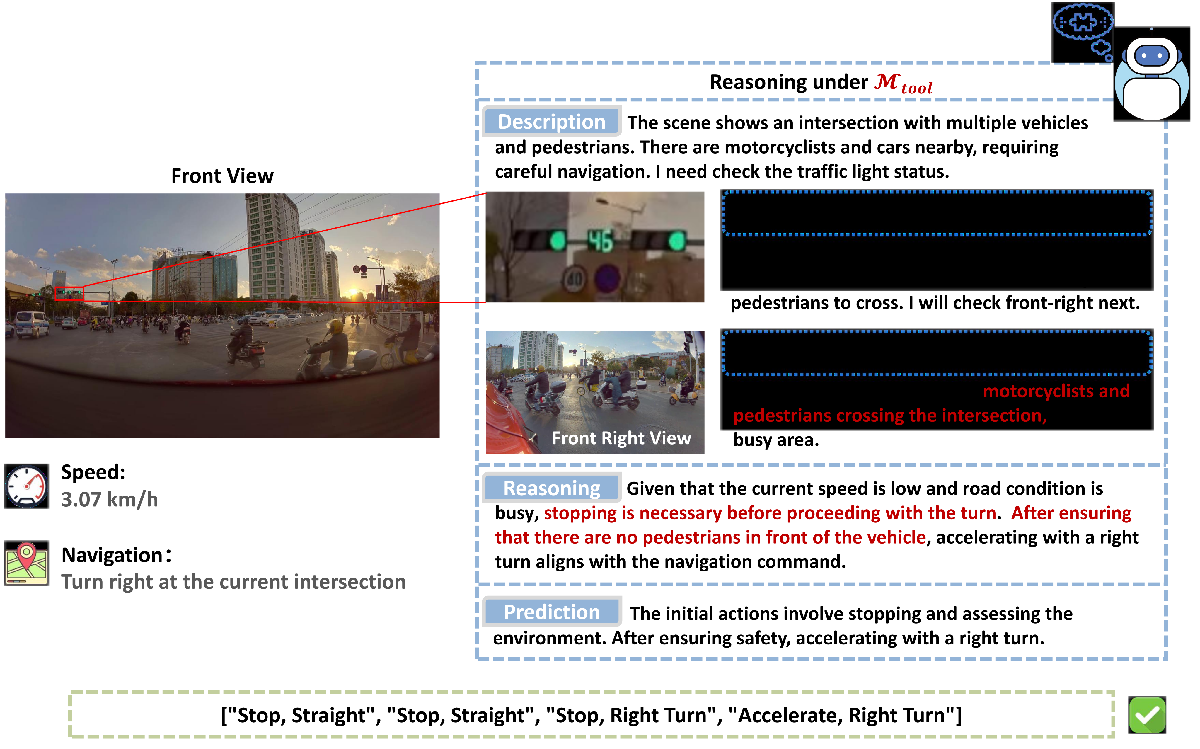
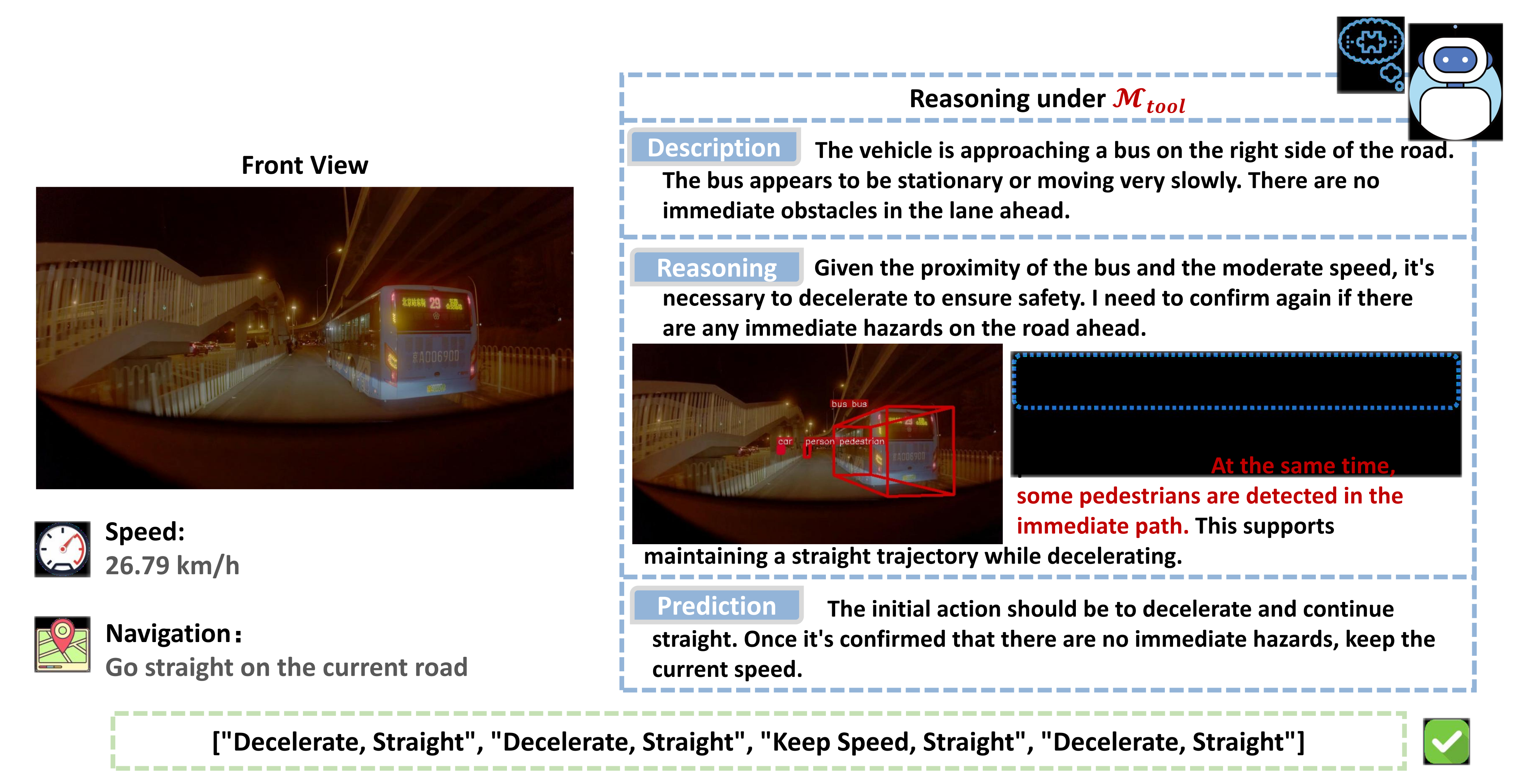
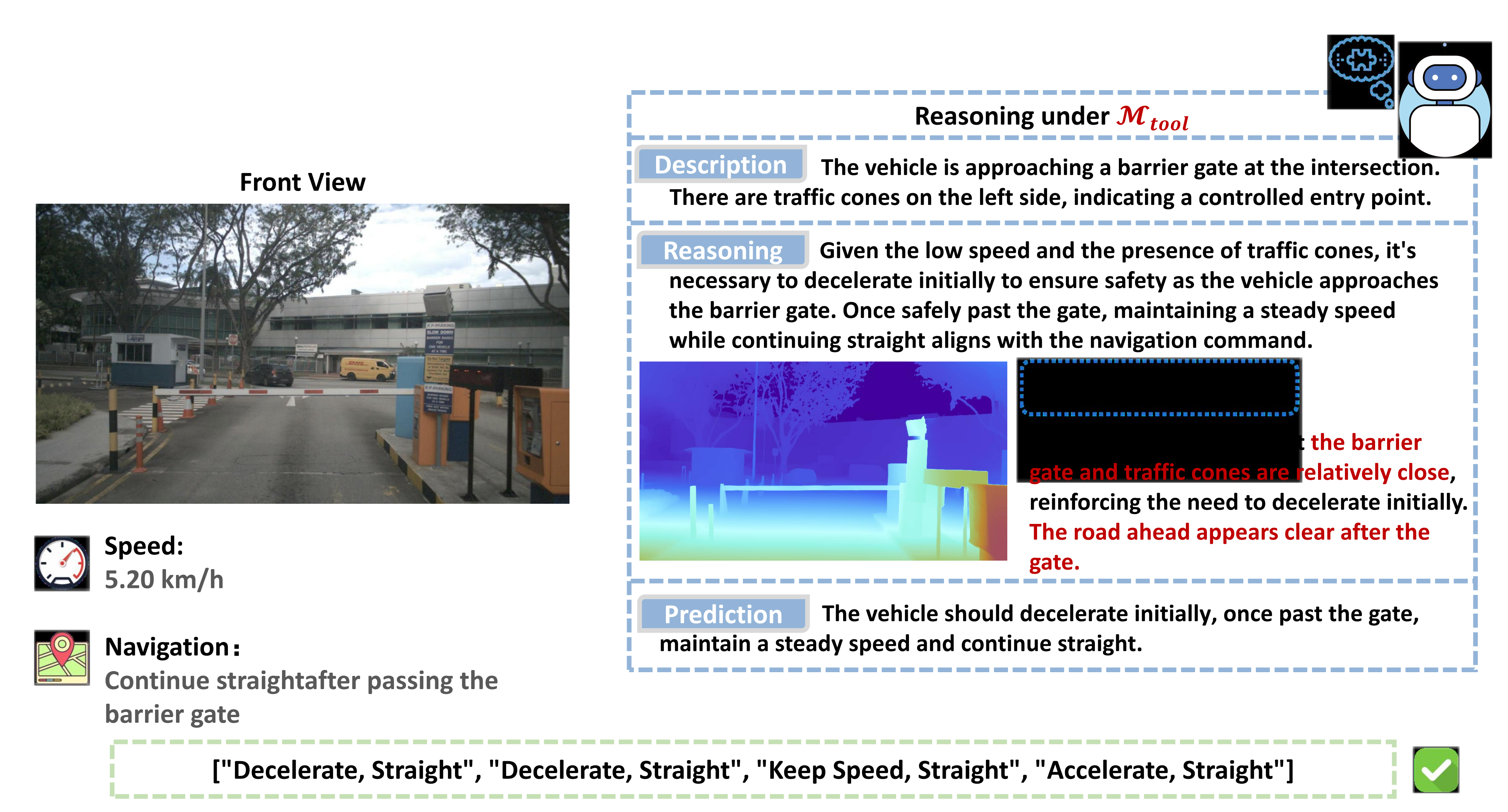
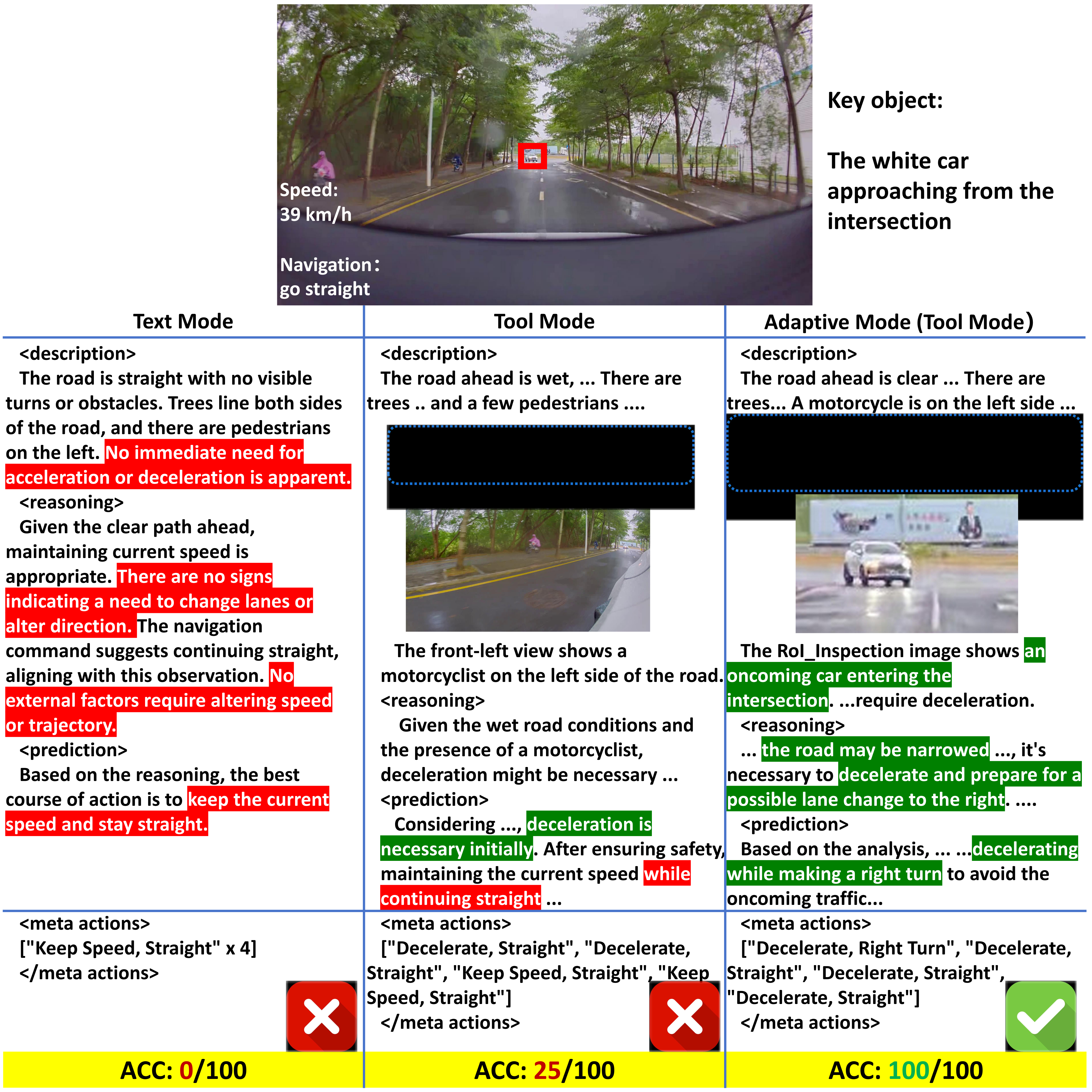
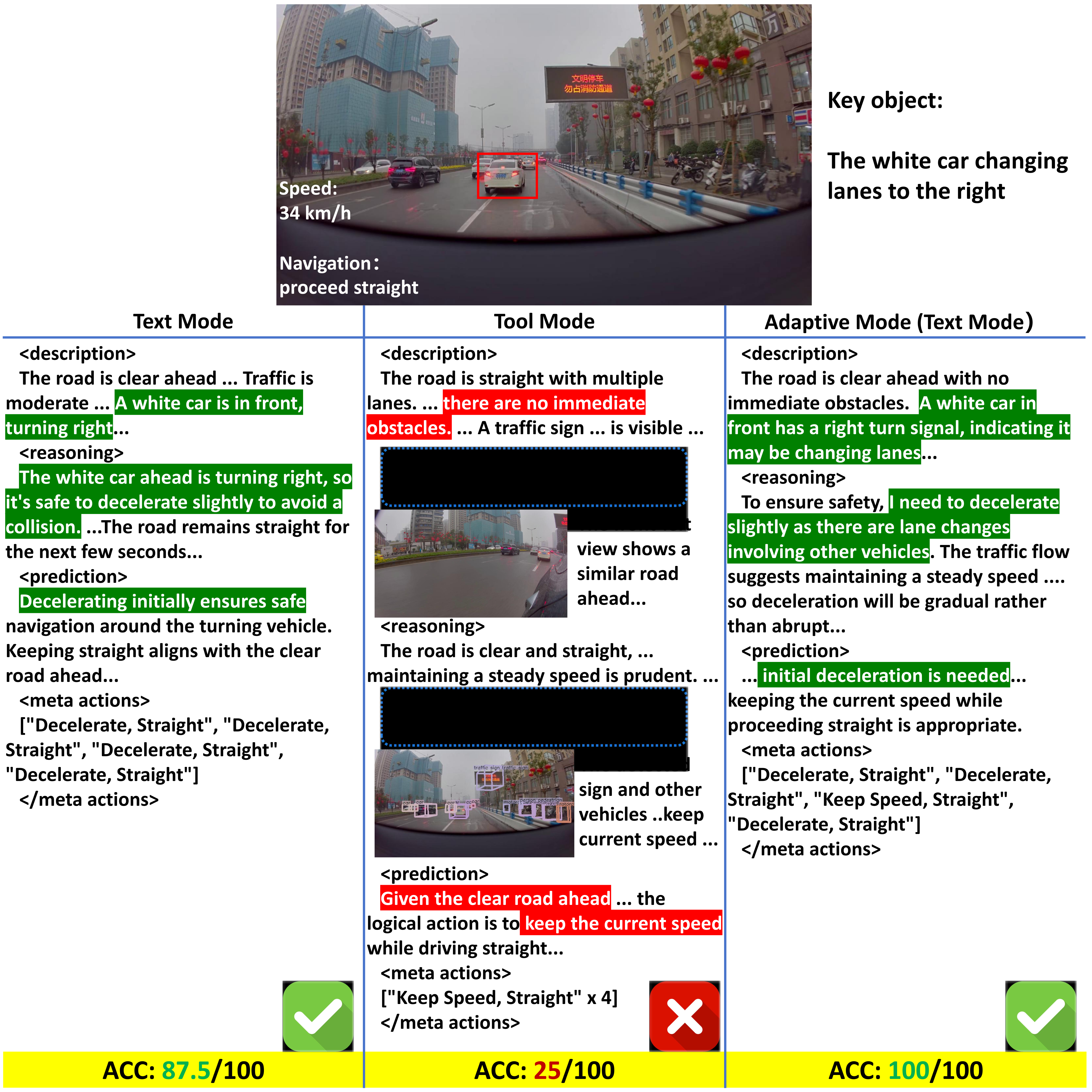
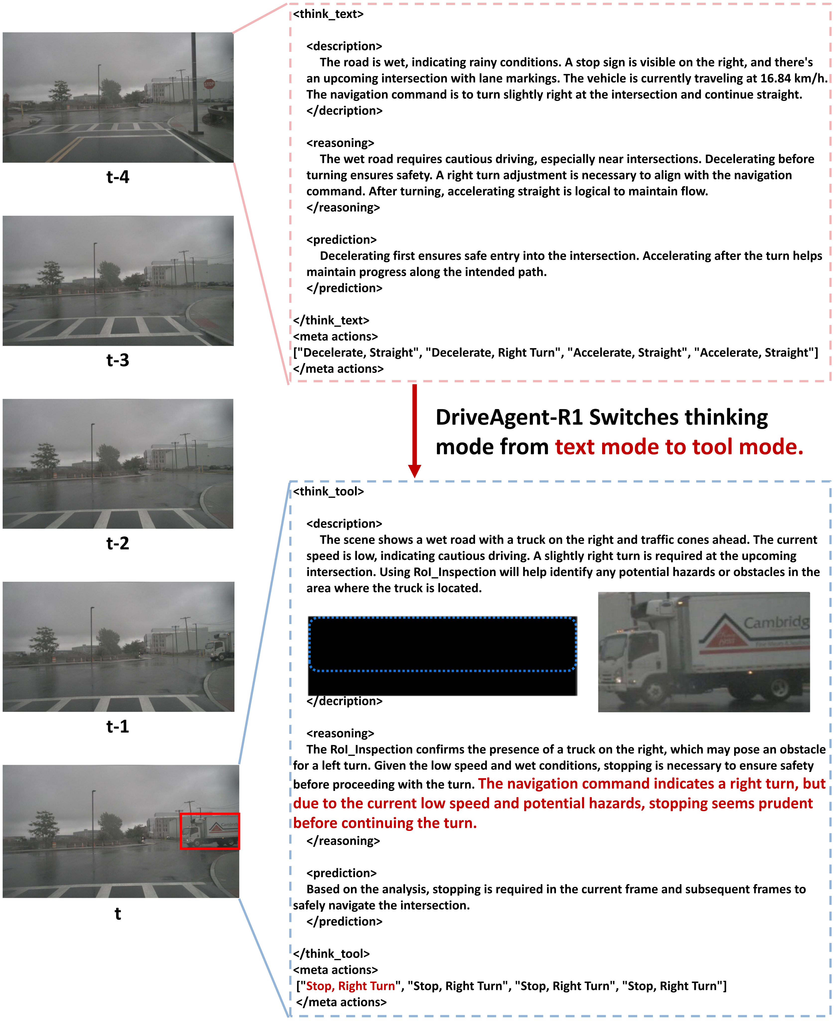
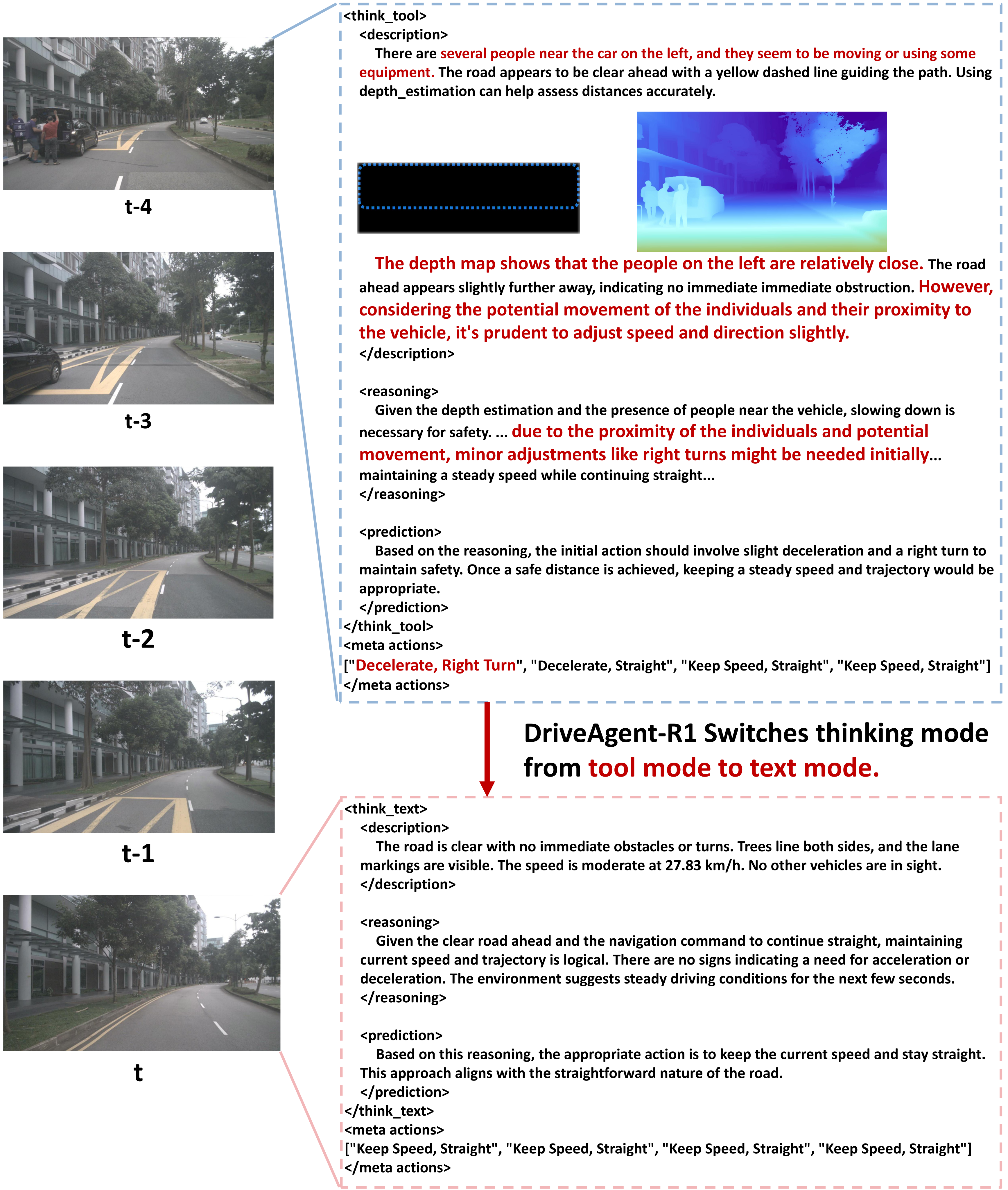
The complete example series illustrates no-tool reasoning for simple roads and toll booths, crop/view inspection for crossing traffic, detection in darkness, depth near barriers, and zooming toward distant pedestrians. Comparative cases show both unfocused tool use and unnecessary tools causing errors. These selected traces explain intended behavior; they do not establish its frequency or causal faithfulness across the test set.
A.11 Analysis of a Failure Case in Complex Intersections
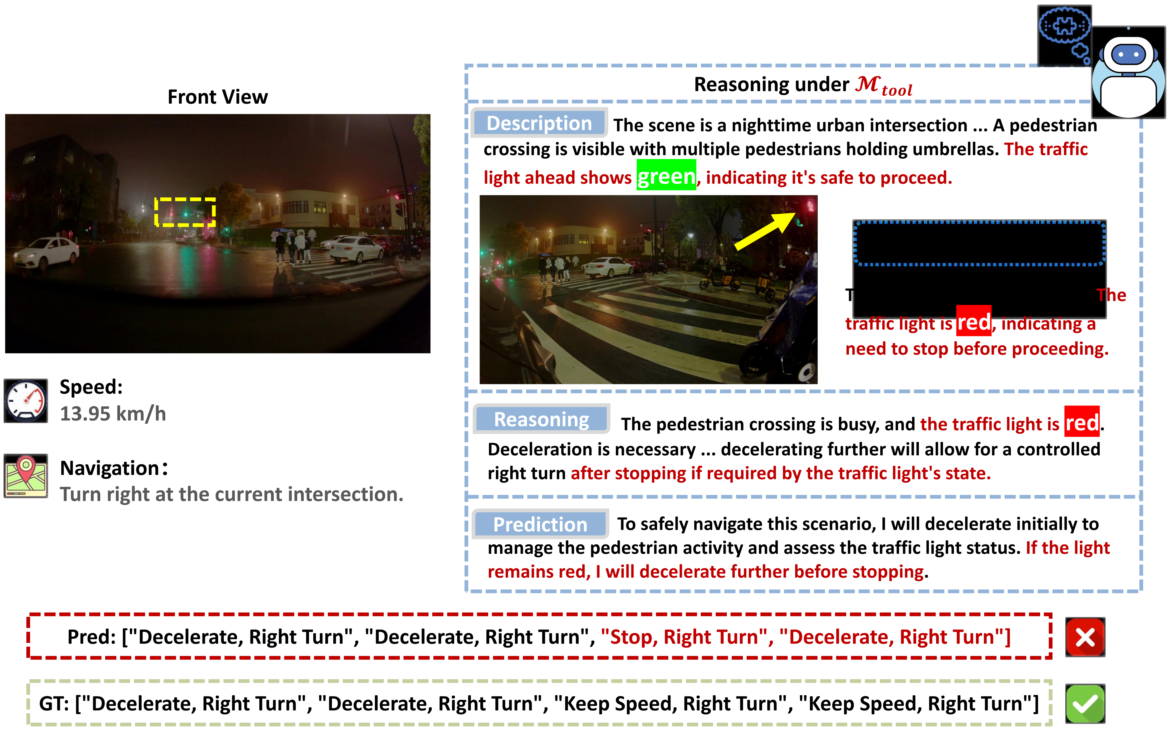
In the failure example, the initial front view correctly shows a green vehicle signal. After requesting another view, the model mistakes a red pedestrian signal for its own and plans an unnecessary stop. Extra evidence can therefore reduce correctness. Proposed remedies include topology/rule knowledge and training on conflicting or ambiguous observations.
A.12 Dynamic Mode Switching Analysis
Two sequences illustrate mode changes as observations evolve: approaching a truck triggers tool use and a more cautious plan, while passing nearby pedestrians lets the model return to no-tool reasoning. The figures show decisions at successive observations, not evidence that a single reasoning rollout arbitrarily changes its initial mode contract.
A.13 Comparision with Instruction-Guide Attention
A generic instruction to attend to a region can reweight existing visual tokens, whereas cropping a high-resolution buffer supplies newly encoded detail. The distinction is meaningful when global encoding loses small-object information; its practical value also depends on correctly selecting the crop.
A.13.1 Quantitative Analysis
In the restricted crop comparison, baseline first-frame/sequence scores are 45.27/43.29; generic textual attention gives 46.72/43.83, and active region inspection gives 48.81/44.65. The reported +3.54/+1.36 gains are over the baseline. Relative to textual attention, the gains are +2.09/+0.82. This single generic-prompt comparison does not exhaust possible attention prompting strategies.
| Inference Setting | First-Frame Joint Acc. | Seq. Avg. Joint Acc. |
| Baseline () | 45.27 | 43.29 |
| Instruction-Guided Attention | 46.72 | 43.83 |
| Active Perception (RoI) | 48.81 | 44.65 |
A.13.2 Qualitative Analysis
The retained example contrasts a missed distant red signal under generic prompting with its recognition after a high-resolution crop, changing the predicted actions toward stopping. It illustrates the information-gain mechanism and remains a selected qualitative case.