At a glance
Intuition: pretrain a model to forecast the meaningful visual features of ordinary videos, then add action inputs when using it as a controller. DINO-world freezes DINOv2 and learns a causal predictor of future patch features on roughly 66 million unlabeled videos. It accepts explicit timestamps, so prediction intervals can vary. Dense forecasting and intuitive-physics tests probe the learned dynamics, while action-conditioned fine-tuning supports planning in three simulated environments. This is a direct frozen-feature companion to JEPA, not a jointly learned JEPA encoder. Its deterministic predictions become inaccurate at longer horizons, and physics plausibility scores are not proof of general physical reasoning. The large private training corpus and simulation-only planning limit reproduction and deployment claims.
1 Introduction
Predicting every pixel spends capacity on details that may not matter for decisions. This work instead starts from an image representation already trained to capture semantics and geometry, then uses video to learn temporal evolution. Large-scale video pretraining and small action-conditioned adaptation are separate stages. That separation reduces the need for action-labeled videos but does not remove it for control.
2 Related work
The paper uses world model broadly for temporal prediction, with or without action inputs. It distinguishes predicting observations, predicting features and using those predictions to select behavior. These capabilities should be evaluated separately.
2.1 Applications
A world model can train a policy in imagined experience, search actions online, generate videos or forecast labels such as segmentation and depth. Strong performance on one use does not guarantee another. Here forecasting and physics provide representation diagnostics, while the final experiments explicitly test action-conditioned planning.
2.2 Design choices
Frozen foundation features avoid jointly learning perception and dynamics from scratch. Unconditional video pretraining uses plentiful videos, while later action blocks adapt the predictor to limited labeled trajectories. The tradeoff is dependence on what the original encoder retains. Comparisons with generative systems involve different training data, objectives and compute.
3 Method
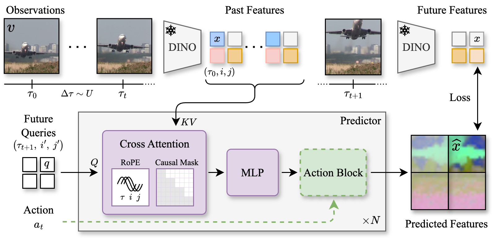
A frozen frame encoder supplies spatial patch tokens. A timestamp-conditioned cross-attention predictor forecasts future tokens from past tokens. Added action blocks adapt that same predictive architecture to controlled trajectories. No pixel decoder is required by this model.
3.1 Observations and state space
Each observation has both an image and a time in seconds. DINOv2 converts it to a feature grid. A prediction query specifies the desired future time and patch position, allowing the model to request one part of a future feature map. Explicit timestamps distinguish, for example, the same visual motion sampled at different frame rates. Architectural flexibility does not guarantee accurate extrapolation to arbitrary times.
Equation 1
| (1) |
3.2 Predictor architecture and training
A learned query attends to past patch features through successive transformer blocks. Three-axis rotary encodings carry time, horizontal position and vertical position. A causal mask prevents future observations leaking into a prediction. Smooth L 1 loss matches every next-frame patch to its frozen target, and teacher forcing permits parallel training. Random time gaps expose the predictor to different forecast intervals; rollout still feeds back its own imperfect predictions.
Equations 2–4
| (2) | ||||
| (3) |
| (4) |
3.3 Action-conditioned fine-tuning
Each new residual action block combines an action embedding with a prediction query. Zero initialization initially leaves the pretrained computation unchanged. Fine-tuning can update only these blocks or the full predictor. This provides a way to reuse video knowledge without requiring the original unlabeled videos to contain action annotations.
4 Experiments
The main setup uses a frozen DINOv2 base encoder, a 1.1-billion-parameter predictor and a large private collection of uncurated videos. Forecasting probes use trained linear output heads; planning uses separate per-environment action fine-tuning. Smaller open video datasets are studied as controls but do not reproduce the scale or diversity of the main corpus.
4.1 Dense feature forecasting and intuitive physics
Forecasting predicts segmentation or depth roughly 0.2 or 0.5 seconds ahead. DINO-world performs strongly on VSPW, while domain-specialized DINO-Foresight is better on some Cityscapes and KITTI settings. Physics tests rank plausible versus implausible videos by prediction surprise. The authors treat those noisy scores as sanity checks, not comprehensive evidence of physical understanding. Encoder quality, head training and prediction quality all affect the measurements.
| VSPW mIoU () | Cityscapes mIoU () | KITTI RMSE () | ||||||||
| Encoder | Present | Short | Mid | Present | Short | Mid | Present | Short | Mid | |
| Copy Last | ViT-B | 52.8 | 47.9 | 42.1 | 68.6 | 53.2 | 39.7 | 2.963 | 3.778 | 4.745 |
| COSMOS-4B | ViT-B | 52.8 | 46.6 | 40.2 | 68.6 | 55.4 | 46.2 | 2.963 | 4.178 | 4.742 |
| COSMOS-12B | ViT-B | 52.8 | 46.6 | 40.7 | 68.6 | 55.6 | 45.9 | 2.963 | 4.157 | 4.617 |
| V-JEPA | ViT-L | 29.1 | 08.2 | 07.7 | 48.8 | 15.5 | 14.0 | 3.502 | 7.217 | 7.491 |
| V-JEPA | ViT-H | 28.0 | 04.9 | 04.6 | 49.7 | 13.3 | 12.2 | 3.402 | 5.458 | 5.785 |
| DINO-Foresight | ViT-B | 50.6 | 44.7 | 37.7 | 66.9 | 64.5 | 57.2 | 2.882 | 3.562 | 3.740 |
| DINO-world | ViT-B | 52.8 | 51.6 | 47.0 | 68.6 | 64.7 | 55.1 | 2.963 | 3.214 | 4.268 |
| Encoder | Predictor | IntPhys | GRASP | InfLevel | |
|---|---|---|---|---|---|
| COSMOS-4B | VAE | 4B | 99.5 | 60.1 | 44.8 |
| V-JEPA | ViT-L | 022M | 92.2 | 67.0 | 58.9 |
| V-JEPA | ViT-H | 022M | 89.4 | 73.0 | 59.9 |
| DINO-Foresight | ViT-B | 193M | 87.8 | 64.9 | 62.8 |
| DINO-world | ViT-B | 1.1B | 91.3 | 76.0 | 63.7 |
4.2 Ablation studies
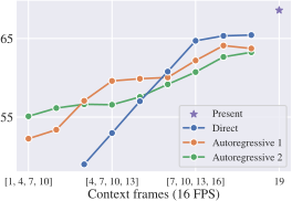
Larger predictors and the broad video corpus improve the tested metrics. Alternative encoders perform worse in the reported configurations, but these comparisons also vary representation geometry and capacity requirements. Direct prediction is better at short intervals; intermediate autoregressive steps help farther ahead, yet forecasting becomes inaccurate near one second. The deterministic model tends to blur uncertain futures rather than explicitly representing multiple possibilities.





| Model | PushT | Wall | PointMaze |
|---|---|---|---|
| Scratch | 46.9 | 87.1 | 59.4 |
| Action-only | 49.4 | 91.1 | 61.6 |
| Fine-tuned | 59.4 | 93.8 | 68.7 |
4.3 Action-conditioned fine-tuning and planning evaluations
Action adaptation improves planning relative to training a predictor from scratch. These experiments use the smaller base predictor, RGB images and actions in Push-T, Wall and PointMaze, evaluated over 512 episodes each. Full fine-tuning outperforms training action blocks alone. The evaluation executes an entire 25-action plan without replanning, so these scores are not interchangeable with closed-loop MPC results from other papers.
5 Conclusion
The study supports reusable latent video prediction followed by action adaptation. It also exposes the remaining gap between short-term feature forecasting and dependable long-horizon control. Stochastic futures, curated data, real-world planning and language conditioning are future work.
Appendix A Implementation and training
A.1 Architecture
Video encoder.
The main encoder produces a grid of 768-dimensional patch tokens; its global classification token and register tokens are discarded. Alternative SigLIP and VAE encoders need representation adjustments. The predictor therefore learns in a particular pretrained feature space rather than a shared universal state space.
Unconditional predictor.
Input and output projections connect encoder dimensions to the cross-attention stack. Rotary position encoding uses separate groups of dimensions for time and two spatial axes, leaving four dimensions unchanged in each head. Relative spatial coordinates support changing resolution, while timestamps retain real temporal units.
Equation 5
| (5) |
Action blocks.
Action embeddings enter residual MLP blocks after each transformer block. Their initial zero layer scales preserve the pretrained model, then learning gives actions an effect. Adding these blocks increases base-model parameters by about 22 million.
A.2 Optimization
Training objective.
Smooth L 1 behaves quadratically for small errors and linearly for larger ones. It is applied elementwise to predicted and target patch features with transition parameter 0.1. This is feature regression, not a probability distribution over possible next frames.
Equation 6
| (6) |
Hyperparameters.
Training uses AdamW, a warmup to a constant learning rate and fixed weight decay. The appendix reports little benefit from the tested schedule alternatives. These are implementation choices, not required properties of frozen-feature prediction.
Compute resources.
The base, large and giant predictors contain 86 million,304 million and 1.1 billion parameters. Training uses multi-node H100 systems; the table distinguishes nodes from GPUs, with eight GPUs per node. Resource efficiency is relative to the compared large generative models, not a claim that the main training is inexpensive.
| Embedding | Blocks | Heads | MLP ratio | Params. | Num. nodes | Training hours | |
|---|---|---|---|---|---|---|---|
| Base | 0768 | 12 | 12 | 4.0 | 086M | 04 | 45.3 |
| Large | 1024 | 24 | 16 | 4.0 | 304M | 08 | 70.2 |
| Giant | 1536 | 40 | 24 | 4.0 | 01.1B | 16 | 95.6 |
Appendix B Datasets
Pre-training datasets.
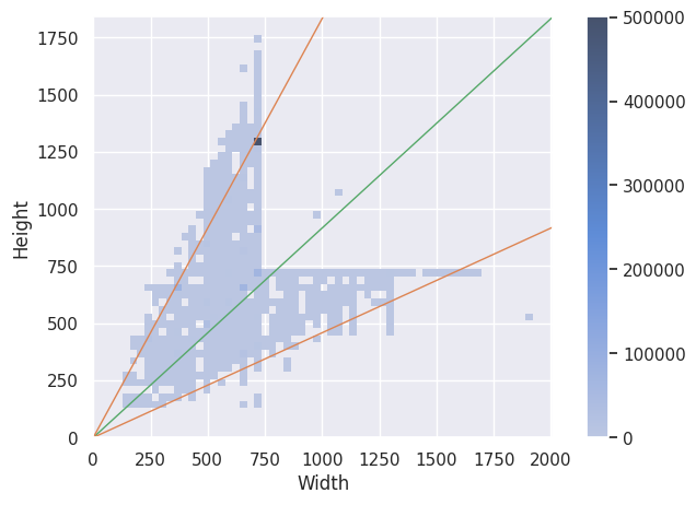
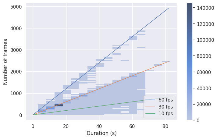
The main dataset contains roughly 66 million videos across varied activities, durations, resolutions and frame rates. Its private status limits exact reproduction. Cityscapes and Something-Something V 2 provide smaller public comparisons, but size and content diversity change together, so their results do not isolate either factor alone.
| Domain | Num. videos | Duration (s) | FPS | Resolution () | |
|---|---|---|---|---|---|
| Cityscapes | Driving | 002,975 | 2 | 16 | |
| SSv2 | Object manipulation | 168,913 | 2–6 | 12 | – |
| Ours | General | 00066M | 5–60 | 10–60 | Misc. |
Figures and assets.
The paper identifies the provenance of displayed videos and states that none of the illustrated clips are in the pretraining dataset. Those figures are retained as source evidence rather than substituted with newly generated examples.
Appendix C Unconditional world model evaluations
C.1 Evaluation datasets
Cityscapes.
Cityscapes has one annotated frame per sequence. The evaluation selects earlier context frames and forecasts that fixed target at short or mid-range intervals. Consequently, each sequence supplies one labeled evaluation case rather than labels for every generated frame.
VSPW.
VSPW annotates every frame, allowing multiple overlapping subsequences per video. Its short and mid-range intervals are 200 and 600 milliseconds in this protocol. Different sampling and class sets matter when comparing its scores with Cityscapes.
KITTI.
KITTI evaluates monocular depth at 200- and 600-millisecond prediction intervals after specified cropping and resizing. A lower depth RMSE is better. It measures future depth estimation, not direct downstream vehicle-control performance.
C.2 Baseline models
COSMOS.
COSMOS has fixed image size, restricted context lengths and a fixed output frame rate. Its evaluation must select suitable generated frames rather than querying an arbitrary timestamp. Those constraints introduce a protocol difference from DINO-world.
DINO-Foresight.
DINO-Foresight predicts compressed features from several intermediate encoder layers at a trained image shape. The protocol reverses its PCA projection and selects compatible features before applying a task head. This differs from predicting only DINOv2’s final-layer features.
V-JEPA.
V-JEPA’s online and target encoders play different roles: present-time heads use normalized target features, while future prediction uses the online encoder and predictor. Tubelet grouping and position interpolation require additional handling. Its predictor was trained as a representation-learning head, so this forecasting adaptation should not be treated as its original training objective.
Equation 7
| (7) | ||||
C.3 Evaluation protocols
DINOv2 dense prediction heads.
Linear segmentation and depth heads are trained on actual present-time encoder features, then applied to predicted future features. Sliding windows and upsampling handle dense outputs. This tests whether predicted features remain useful for a downstream head, separating feature prediction from training a specialized future-label decoder.
DINO-Foresight on Cityscapes.
For DINO-Foresight, the head is trained on features processed through its PCA compression and inverse. This yields better results than using untouched final-layer features. The paper therefore uses a baseline-compatible head protocol rather than assuming all feature spaces are identical.
COSMOS on Cityscapes.
COSMOS receives selected context frames, generates a sequence, and the corresponding future frame is encoded with DINOv2 before segmentation. Resizing, padding and frame selection align it with the labeled target. Its short and mid-range predictions are both generated autoregressively.
COSMOS on VSPW.
The VSPW protocol uses overlapping valid subsequences and resizes generated frames to the segmentation head’s expected scale. This follows its denser annotation structure rather than copying Cityscapes sampling unchanged.
COSMOS on KITTI.
KITTI similarly removes padding and resizes COSMOS output to match the depth head. The reported result includes this generation-to-encoding evaluation pipeline.
DINO-Foresight on KITTI.
DINO-Foresight’s positional encoding is interpolated for KITTI’s wide frame shape, and the head uses PCA-processed features. These adaptations are necessary to compare a fixed-shape predictor on the depth benchmark.
V-JEPA on Cityscapes.
Using target-encoder features for head training improves V-JEPA forecasting scores relative to online-encoder features. The protocol assumes the predictor is aligned with those target features. Head choice materially affects a comparison of world-model representations.
Appendix D Action-conditioned fine-tuning and planning
D.1 Environments
Action fine-tuning reuses DINO-WM’s released simulated trajectories. This study ignores proprioception and uses only RGB observations and recorded actions. Its control input is therefore narrower than some later world-model comparisons.
Push-T.
Push-T uses noisy replays of expert-derived trajectories. Both the pusher and object must match the target configuration. The presence of action-labeled, expert-derived data should remain visible when interpreting the training requirements.
Point Maze.
PointMaze uses random trajectories but retains inertia and acceleration, so temporal evidence is necessary for predicting motion. It is simulated image-based navigation.
Wall.
Wall has two rooms and a doorway, with random movement trajectories. The retained dataset table records trajectory counts and lengths separately for all three tasks.
| Resolution | Num. trajectories | Traj. length | |
|---|---|---|---|
| PointMaze | 224 | 02000 | 100 |
| Push-T | 224 | 18500 | 100-300 |
| Wall | 224 | 01920 | 50 |
D.2 Action-conditioned fine-tuning.
A 90/10 trajectory split separates fine-tuning from planning evaluation. One prediction consumes a chunk of five actions and skips intermediate image observations. Skipping frames is not stacking them as additional evidence. The comparison tests from-scratch training, frozen-predictor action blocks and full predictor fine-tuning.
D.3 Planning algorithm
Planning evaluation.
A plan minimizes the final predicted feature distance to a supplied goal image. The horizon is 25 physical actions but only five predictor calls because actions are chunked in groups of five. Goals are selected to be reachable within that horizon. All actions execute without feedback replanning in the reported evaluation.
Equation 8
| (8) |
Cross-Entropy Method.
CEM samples 300 candidate sequences per iteration and fits its Gaussian proposal to the ten best, repeating for thirty iterations. All 25 actions are then executed. Although the generic procedure permits executing a shorter prefix, the actual hyperparameters choose the full horizon; this is open-loop planning, not repeated MPC feedback.
Equation 9
| (9) |
| Push-T | 300 | 25 | 5 | 5 | 25 | 10 | 30 |
|---|---|---|---|---|---|---|---|
| PointMaze | 300 | 25 | 5 | 5 | 25 | 10 | 30 |
| Wall | 300 | 25 | 5 | 5 | 25 | 10 | 30 |
Appendix E Results
E.1 Qualitative visualizations
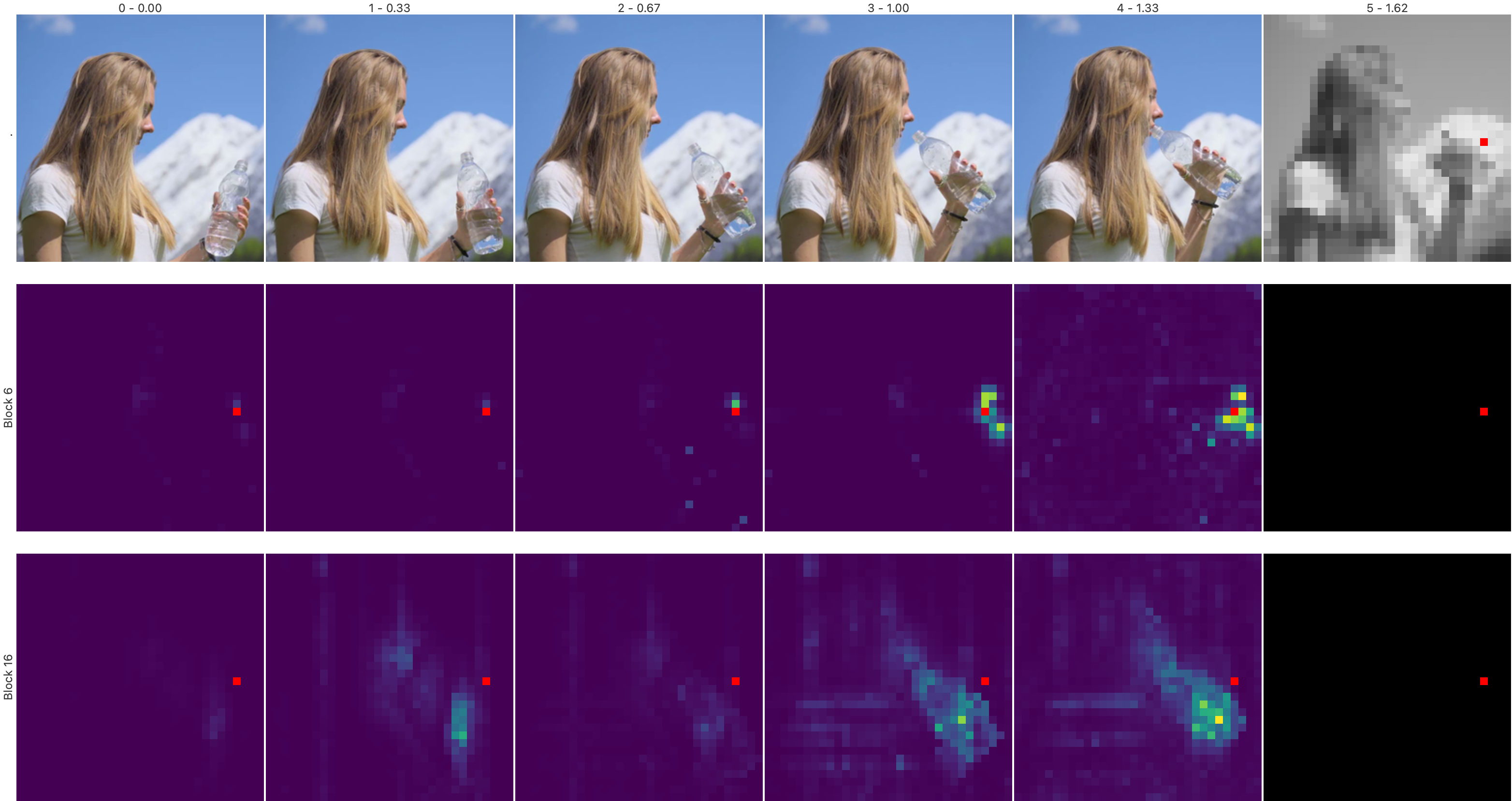
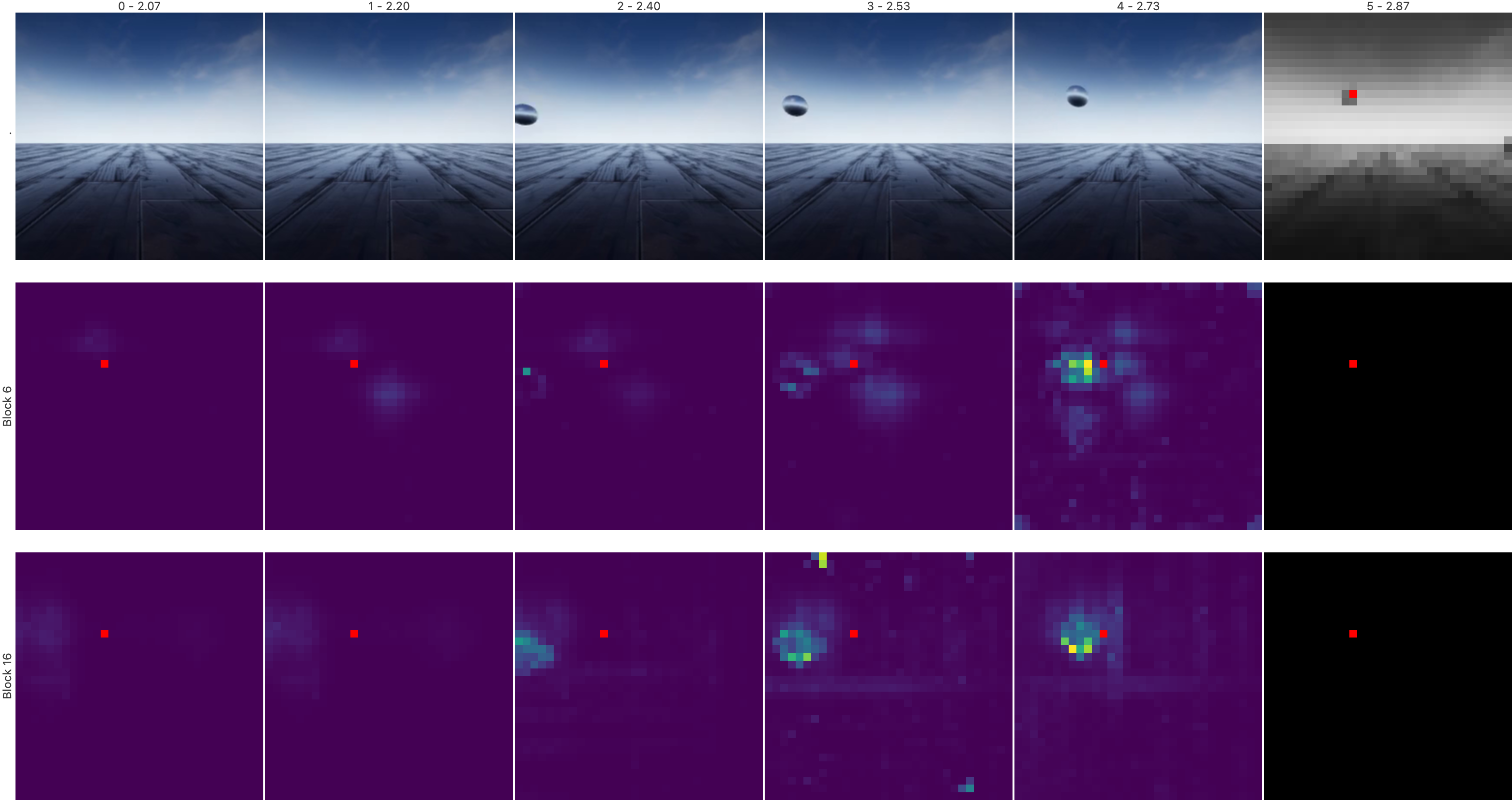
Feature-color visualizations use a PCA projection fitted to encoder features. They show plausible local motions and increasing blur as rollout uncertainty grows. Selected attention maps suggest tracking of previous object locations, but attention inspection alone does not establish an object-centric causal mechanism.




E.2 Intuitive physics
The category tables reveal uneven intuitive-physics performance beneath average scores. Some categories are near perfect while others remain near chance or worse. These diagnostics support a limited plausibility capability, not universal understanding of permanence, gravity or solidity.
| Encoder | Collision | Continuity | Gravity | Gravity | Gravity | Gravity | Gravity | Inertia | Inertia2 | |
|---|---|---|---|---|---|---|---|---|---|---|
| Continuity | Inertia | Inertia2 | Support | |||||||
| DINO-Foresight | ViT-B | 00.0 | 71.1 | 73.4 | 46.1 | 14.8 | 53.1 | 100.0 | 44.5 | 60.2 |
| V-JEPA | ViT-L | 54.7 | 47.7 | 55.5 | 64.1 | 75.0 | 53.1 | 100.0 | 47.7 | 53.9 |
| V-JEPA | ViT-H | 28.9 | 53.9 | 58.6 | 71.9 | 78.9 | 56.2 | 100.0 | 52.3 | 68.0 |
| COSMOS | 4B | 56.3 | 51.6 | 56.3 | 57.0 | 89.8 | 51.6 | 100.0 | 48.4 | 46.1 |
| DINO-world | ViT-B | 00.0 | 79.7 | 89.1 | 28.9 | 59.4 | 59.4 | 100.0 | 57.8 | 71.1 |
| Object | Object | Object | Solidity | Solidity | Unchangeableness | Unchangeableness2 |
|---|---|---|---|---|---|---|
| Permanence | Permanence2 | Permanence3 | Continuity | Continuity2 | ||
| 100.0 | 46.9 | 99.2 | 71.9 | 83.6 | 100.0 | 73.4 |
| 027.3 | 82.0 | 99.2 | 87.5 | 60.9 | 091.4 | 71.9 |
| 075.8 | 94.5 | 99.2 | 88.3 | 81.2 | 093.0 | 67.2 |
| 000.0 | 53.9 | 96.9 | 79.7 | 23.4 | 088.3 | 61.7 |
| 100.0 | 83.6 | 99.2 | 96.9 | 93.0 | 100.0 | 98.4 |