At a glance
Online maps can help motion prediction, but adding their uncertainty is not uniformly useful. This method models correlated errors in each map vertex and learns to blend forecasts from predictors with and without uncertainty, using the predicted trajectories themselves as gating input.
Across four map estimators and two predictors on nuScenes, the combined model improves all tabulated accuracy metrics relative to the previous uncertainty method. The headline 23.6% is a relative miss-rate reduction for one pairing, not a universal prediction gain. Code, data and model resources are linked by the authors.
I INTRODUCTION
“Mapless” means constructing local map elements online from sensor data rather than relying on a maintained offline HD map. The downstream predictor must still contend with errors caused by occlusion, distance and imperfect geometry.
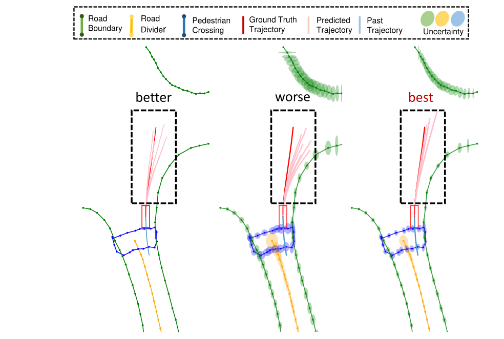
The paper observes that uncertainty helps most when driving kinematics change; steady straight travel or steady turning can favor the baseline. It therefore combines a correlated map-error representation with a learned gate between two prediction streams, rather than always using uncertainty.
II Related Works
The study connects online vector-map estimation with map-informed trajectory prediction, focusing on how uncertainty passes between these modules.
II-A Online Map Estimation
Online mapping has moved from rasterized bird’s-eye semantic maps to learned polylines and polygons, with improvements in geometry, temporal consistency and robustness. Downstream reliability remains a separate concern.
Gu et al. model each vertex with independent horizontal and vertical Laplace errors. This paper introduces within-vertex correlation so the uncertainty ellipse can align with a road element’s orientation.
II-B Map-Informed Trajectory Prediction
Vectorized maps avoid some raster discretization and encode road structure for graph- or transformer-based predictors. HiVT and DenseTNT provide the representative downstream models here.
Previous uncertainty integration concatenates uncertainty with map coordinates. The proposed contribution adds a learned decision about how much to rely on that enriched stream.
III Method
The method first diagnoses uncertainty’s scenario-dependent effect, then combines correlated vertex distributions, dual-stream prediction and trajectory-based gating.
III-A Analysis of Map Uncertainty for Trajectory Prediction
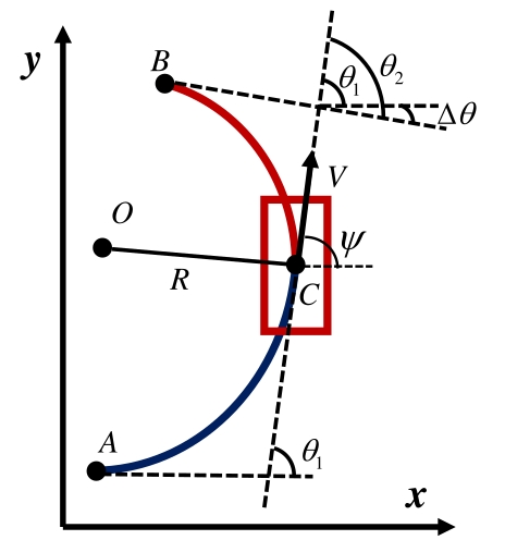
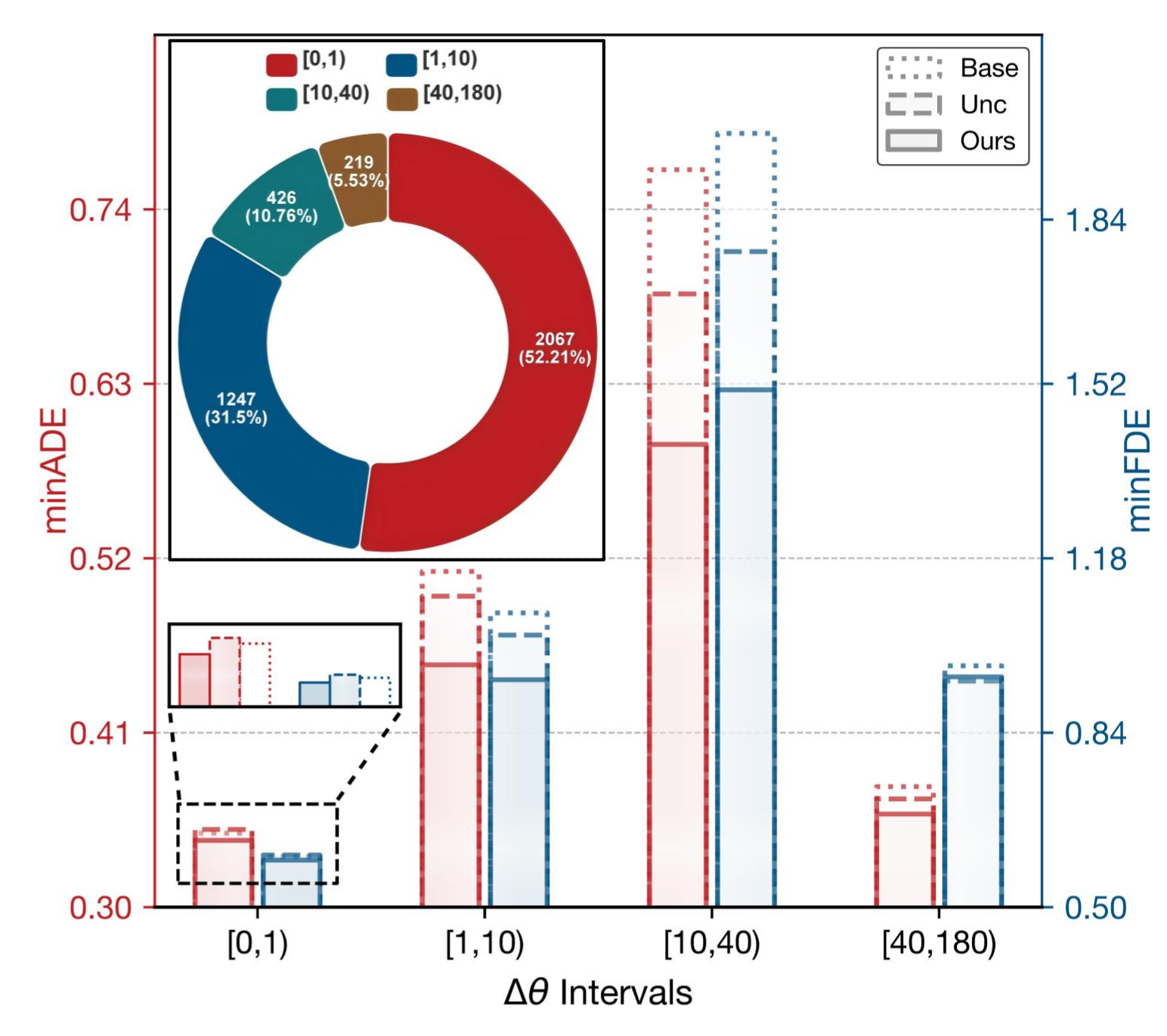
The diagnostic compares average ego heading changes over the past and future two-second windows. Their absolute difference, Δθ, is small for steady straight motion or steady turning; it measures a change in turning behavior, not simply road curvature.
In the [0,1) interval, comprising 52.21% of the analyzed scenes, the baseline slightly outperforms previous uncertainty integration: minADE 0.3466 versus 0.3490 and minFDE 0.5980 versus 0.6016. Larger-change intervals favor uncertainty. This is a dataset association; the future-based diagnostic is not an available ground-truth input at inference.
Equations 1–2
| (1) |
| (2) |
III-B Architecture Overview
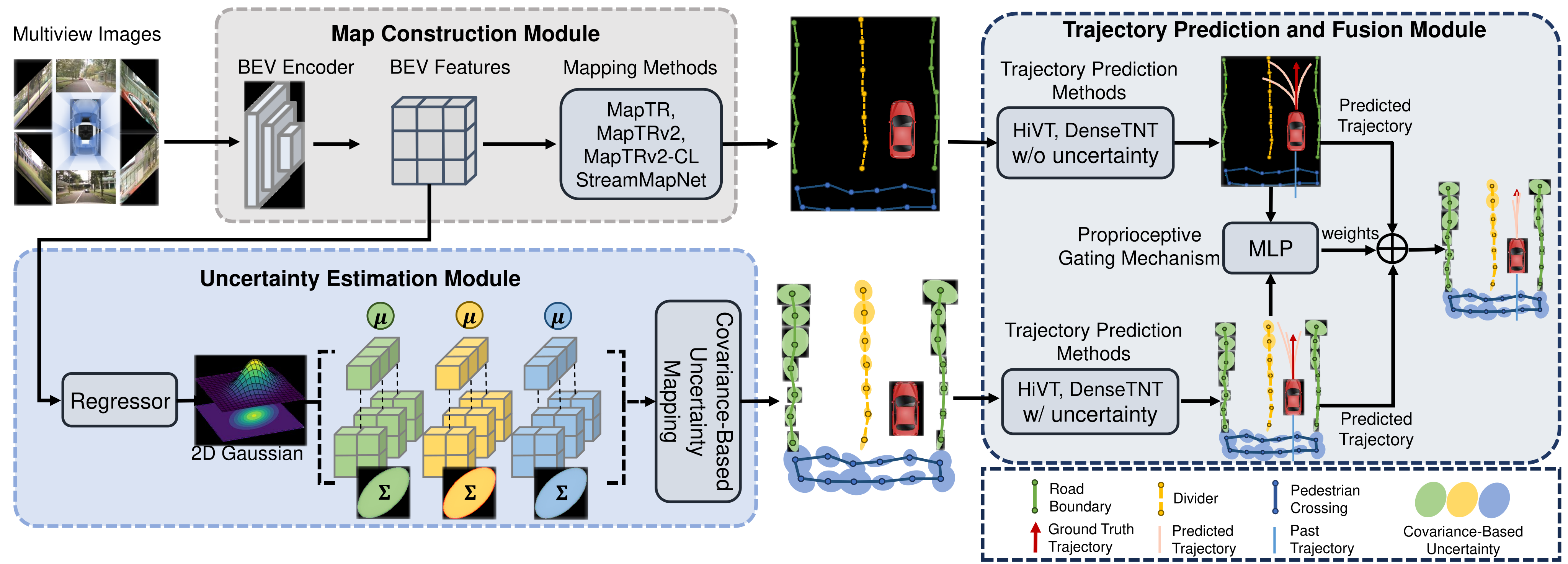
A map estimator predicts vertices and their uncertainty. The baseline stream encodes mean coordinates through an MLP; the enriched stream encodes coordinates concatenated with covariance. Each feeds a trajectory predictor, producing two candidate forecast sets.
A further MLP consumes the predicted trajectories and outputs weights for their combination. The gate operates on predictions carrying implicit kinematic information; it does not receive an extra image or an oracle future trajectory.
III-C Covariance-Based Uncertainty Modeling
Each vertex has a two-dimensional Gaussian with predicted mean, horizontal and vertical variances, and correlation coefficient. The covariance permits tilted error ellipses rather than axis-aligned independent errors. The product likelihood in Equation 3 still factorizes across vertices; it does not model correlations among different map vertices.
The paper argues that Gaussian uncertainty is preferable to Laplace uncertainty, but supplies no general proof of superior outlier robustness. Its distribution ablation supports lower displacement errors for the correlated Gaussian in this setup, with a different miss-rate tradeoff.
Equation 3
| (3) |
III-D Proprioceptive Scenario Gating
Flatten and pad the two streams’ predicted trajectories, concatenate them, and feed an MLP with stated layer sizes 512, 256, 128, 64, 32 and 2. A temperature-scaled softmax produces nonnegative weights summing to one, which blend the streams.
The manuscript’s tensor dimensions are inconsistent: it calls each stream 1×512, the concatenated input 1×2, and describes a 512-to-2 reduction. It also calls the output weights training labels without fully deriving their targets. These details require implementation checks; the original equation is preserved.
Equation 4
| (4) |
III-E Loss Functions
The map regressor minimizes a bivariate Gaussian negative log-likelihood: a covariance log-determinant term plus a Mahalanobis position error, summed over vertices. An additional regularizer is mentioned for stability without a complete formula or coefficient.
The gate uses mean squared error against target mixing weights intended to reflect the better trajectory selection. Although called self-supervised, target construction and covariance-validity parameterization are not fully specified in the text.
Equation 5
| (5) |
IV Experienments
Evaluation combines four online mappers with two trajectory predictors, then separately ablates covariance, gating, visual-input alternatives and a stronger baseline stream.
| Prediction Method | HiVT [2] | DenseTNT [13] | ||||||
|---|---|---|---|---|---|---|---|---|
| Online HD Map Method | minADE | minFDE | MR | FPS | minADE | minFDE | MR | FPS |
| MapTR [4] | 0.4015 | 0.8404 | 0.0960 | 17.91 | 1.1228 | 2.2151 | 0.3726 | 7.36 |
| MapTR [4] + Unc [3] | 0.3910 | 0.8049 | 0.0818 | 16.65 | 1.1946 | 2.2666 | 0.3848 | 7.75 |
| MapTR [4] + Ours | 0.3672 () | 0.7395 () | 0.0756 () | 15.08 | 1.0865 () | 2.0969 () | 0.3728 () | 6.96 |
| MapTRv2 [1] | 0.4017 | 0.8406 | 0.0959 | 15.66 | 1.3262 | 2.5687 | 0.4301 | 7.57 |
| MapTRv2 [1] + Unc [3] | 0.3913 | 0.8054 | 0.0819 | 14.98 | 1.3256 | 2.6390 | 0.4435 | 7.38 |
| MapTRv2 [1] + Ours | 0.3670 () | 0.7538 () | 0.0708 () | 13.65 | 1.1585 () | 2.4566 () | 0.3891 () | 6.89 |
| MapTRv2-CL [1] | 0.3789 | 0.7859 | 0.0865 | 14.02 | 0.8333 | 1.4752 | 0.1719 | 7.62 |
| MapTRv2-CL [1] + Unc [3] | 0.3674 | 0.7418 | 0.0739 | 14.03 | 0.9666 | 1.6439 | 0.2082 | 7.29 |
| MapTRv2-CL [1] + Ours | 0.3659 () | 0.7404 () | 0.0721 () | 13.47 | 0.7787 () | 1.4662 () | 0.1590 () | 6.73 |
| StreamMapNet [5] | 0.3963 | 0.8223 | 0.0923 | 14.17 | 1.0639 | 2.1430 | 0.3412 | 7.42 |
| StreamMapNet [5] + Unc [3] | 0.3899 | 0.8101 | 0.0861 | 13.69 | 1.0902 | 2.1412 | 0.3261 | 6.91 |
| StreamMapNet [5] + Ours | 0.3828 () | 0.7981 () | 0.0834 () | 13.26 | 0.9675 () | 1.6883 () | 0.2628 () | 6.32 |
IV-A Experiment Setup
The stated nuScenes split contains 500 training, 200 validation and 150 test scenes. Each 20-second scene has 2-Hz annotations and six cameras. Models predict three future seconds from two historical seconds and output six candidate trajectories per agent.
minADE and minFDE select the best candidate’s average or final Euclidean error; miss rate counts examples whose best endpoint is more than two meters from ground truth. These oracle-best-of-six metrics do not evaluate selecting a single safe plan or closed-loop driving.
Training uses one RTX 3090. Mapping learning rate is 1.5×10⁻⁴, regression weight 0.03 and gradient-norm clipping 3. Prediction learning rate is 5×10⁻⁴, with HiVT batch size/temperature 32/0.6 and DenseTNT 16/0.5; dropout is 0.1.
IV-B Main Results
Against the previous uncertainty method, MapTRv2–HiVT improves minADE 0.3913→0.3670, minFDE 0.8054→0.7538 and miss rate 0.0819→0.0708. MapTRv2-Centerline–DenseTNT achieves the largest miss-rate reduction, 0.2082→0.1590 (23.6% relative), with 19.4% and 10.8% displacement-error reductions.
Benefits depend on the reference: MapTR–DenseTNT’s miss rate is 0.3728, slightly worse than the no-uncertainty baseline’s 0.3726. Some source percentage annotations are inaccurate—for example StreamMapNet–HiVT’s 0.0861→0.0834 miss-rate change is about 3.1%, not the printed 0.3%. Original table values and annotations remain unchanged.
The full model is slower than the corresponding baseline in Table I, running 13.26–15.08 FPS with HiVT and 6.32–6.96 FPS with DenseTNT on an RTX 3090. The later much higher gating-specific throughput should not be substituted for these system measurements.
IV-C Visualizations
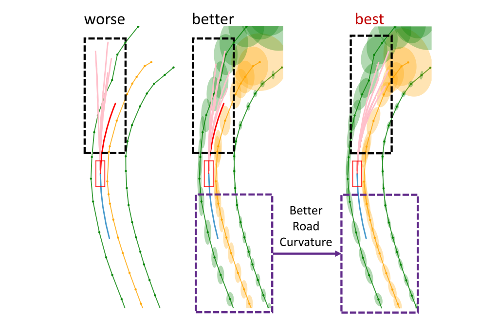
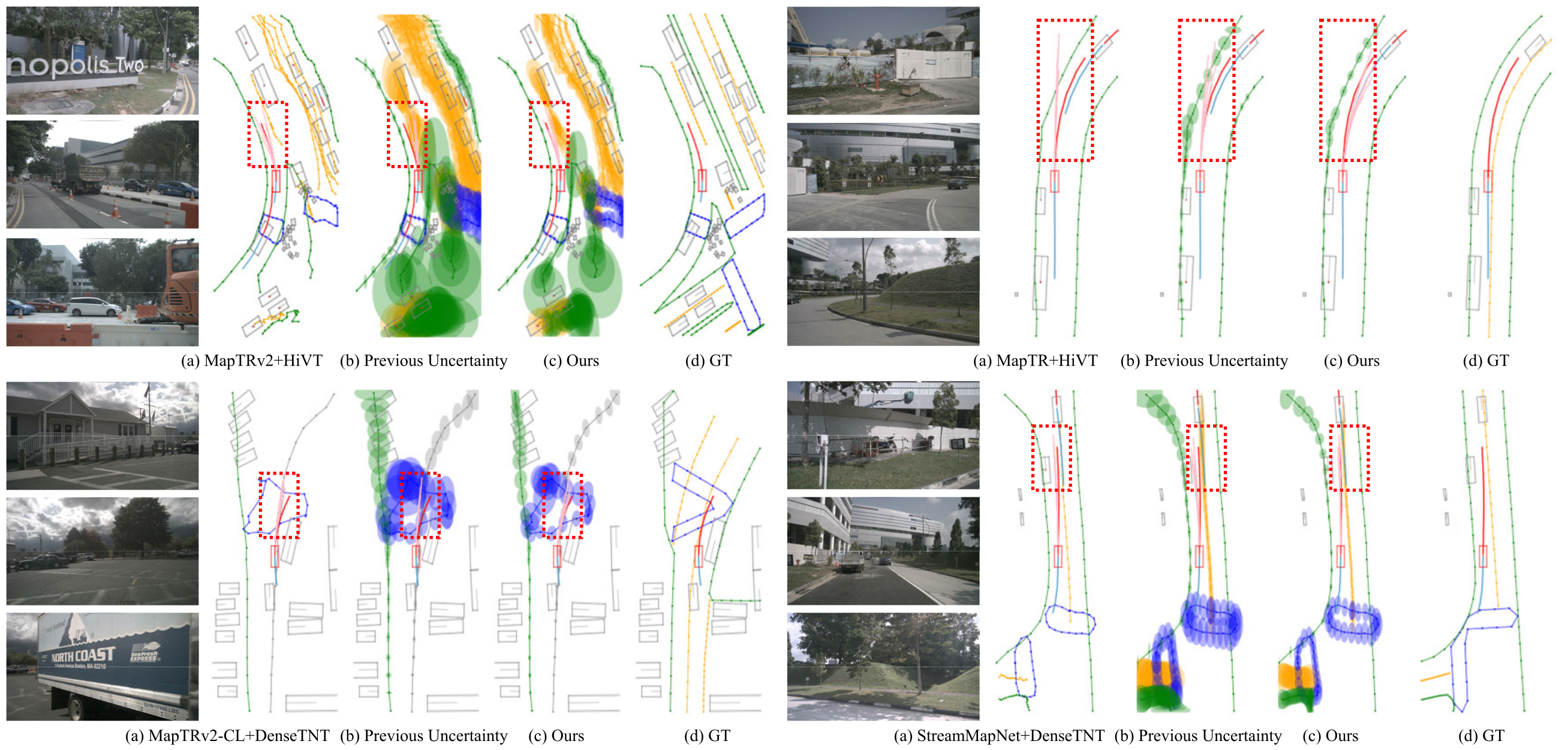
Four selected examples cover a steady turn, approaching a gentle curve, passing a truck and transitioning from turning to straight motion. The combined predictions follow the ground-truth path more closely than the illustrated alternatives, sometimes avoiding their excursions beyond lane boundaries.
These are offline forecast visualizations, not demonstrations that a controlled vehicle safely avoided an obstacle. They complement the aggregate errors without establishing a collision-rate reduction.
IV-D Ablations
Separate ablations test each proposed component and alternative inputs to the gate. They also expose metric tradeoffs hidden by the main headline.
IV-D 1 Covariance-based Map Uncertainty
Covariance alone improves the HiVT results across all four mappers relative to previous uncertainty integration. The 4.3% minFDE reduction belongs to MapTRv2, not MapTRv2-Centerline as the prose states; StreamMapNet miss rate falls 0.0861→0.0805.
With MapTR, correlated Gaussian gives the lowest minADE/minFDE, 0.3851/0.7812, but its 0.0815 miss rate is worse than correlated Laplace’s 0.0803 and independent Laplace’s 0.0802. Table III’s independent-Laplace miss rate also differs from the 0.0818 in other tables. The experiment does not show Gaussian dominance on every metric.
| Prediction Method | HiVT [2] | ||
|---|---|---|---|
| Online HD Map Method | minADE | minFDE | MR |
| MapTR [4] | 0.4015 | 0.8404 | 0.0960 |
| MapTR [4] + Unc [3] | 0.3910 | 0.8049 | 0.0818 |
| MapTR [4] + CovMat | 0.3851 () | 0.7812 () | 0.0815 () |
| MapTRv2 [1] | 0.4017 | 0.8406 | 0.0959 |
| MapTRv2 [1] + Unc [3] | 0.3913 | 0.8054 | 0.0819 |
| MapTRv2 [1] + CovMat | 0.3776 () | 0.7707 () | 0.0789 () |
| MapTRv2-CL [1] | 0.3789 | 0.7859 | 0.0865 |
| MapTRv2-CL [1] + Unc [3] | 0.3674 | 0.7418 | 0.0739 |
| MapTRv2-CL [1] + CovMat | 0.3662 () | 0.7411 () | 0.0728 () |
| StreamMapNet [5] | 0.3963 | 0.8223 | 0.0923 |
| StreamMapNet [5] + Unc [3] | 0.3899 | 0.8101 | 0.0861 |
| StreamMapNet [5] + CovMat | 0.3843 () | 0.8035 () | 0.0805 () |
| Prediction Method | HiVT [2] | ||
|---|---|---|---|
| Online HD Map Method | minADE | minFDE | MR |
| MapTR [4] | 0.4015 | 0.8404 | 0.0960 |
| MapTR [4] + Bivariate Laplace w/o Covariance [3] | 0.3910 | 0.8049 | 0.0802 |
| MapTR [4] + Bivariate Gaussian w/o Covariance | 0.3931 | 0.8079 | 0.0839 |
| MapTR [4] + Bivariate Laplace w/ Covariance | 0.3853 | 0.7862 | 0.0803 |
| MapTR [4] + Bivariate Gaussian w/ Covariance (Ours) | 0.3851 | 0.7812 | 0.0815 |
IV-D 2 Proprioceptive Scenario Gating
Gating alone improves every listed HiVT metric over the previous uncertainty method. Average baseline-stream weight is 0.82 in stable scenarios and 0.37 elsewhere, consistent with the diagnostic motivation.
Combining both components is not uniformly better than gating alone: MapTRv2-Centerline–HiVT gating gives minADE/minFDE/MR 0.3650/0.7362/0.0685, compared with the combined model’s 0.3659/0.7404/0.0721. The components interact rather than yielding guaranteed additive gains.
| Prediction Method | HiVT [2] | ||
|---|---|---|---|
| Online HD Map Method | minADE | minFDE | MR |
| MapTR [4] | 0.4015 | 0.8404 | 0.0960 |
| MapTR [4] + Unc [3] | 0.3910 | 0.8049 | 0.0818 |
| MapTR [4] + Gating | 0.3829 () | 0.7855 () | 0.0805 () |
| MapTRv2 [1] | 0.4017 | 0.8406 | 0.0959 |
| MapTRv2 [1] + Unc [3] | 0.3913 | 0.8054 | 0.0819 |
| MapTRv2 [1] + Gating | 0.3815 () | 0.7914 () | 0.0807 () |
| MapTRv2-CL [1] | 0.3789 | 0.7859 | 0.0865 |
| MapTRv2-CL [1] + Unc [3] | 0.3674 | 0.7418 | 0.0739 |
| MapTRv2-CL [1] + Gating | 0.3650 () | 0.7362 () | 0.0685 () |
| StreamMapNet [5] | 0.3963 | 0.8223 | 0.0923 |
| StreamMapNet [5] + Unc [3] | 0.3899 | 0.8101 | 0.0861 |
| StreamMapNet [5] + Gating | 0.3858 () | 0.7981 () | 0.0847 () |
IV-D 3 Dynamic Proprioception vs. Exteroceptive Sensing
The visual alternatives encode a front-camera image with CLIP or ResNet50, then train an MLP using four semantic categories: low/high curvature, other agents and straight road. Both underperform the proposed method in Table V, sometimes falling below the baseline.
These particular semantic-label gates do not establish that every visual or multimodal gating design is inferior. Table VI reports 52.26–92.09 FPS for the proposed gate versus 2.15–2.42 for CLIP and 6.51–6.91 for ResNet50; its approximate 30×/10× caption does not match every table ratio. This is a separate gating comparison from Table I’s slower dual-stream pipeline.
| Prediction Method | HiVT [2] | ||
|---|---|---|---|
| Online HD Map Method | minADE | minFDE | MR |
| MapTR [4] | 0.4015 | 0.8404 | 0.0960 |
| MapTR [4] + CLIP [41] | 0.4200 | 0.8821 | 0.1040 |
| MapTR [4] + ResNet50 [42] | 0.4248 | 0.9008 | 0.1060 |
| MapTR [4] + Ours | 0.3672 | 0.7395 | 0.0756 |
| MapTRv2 [1] | 0.4017 | 0.8406 | 0.0959 |
| MapTRv2 [1] + CLIP [41] | 0.3988 | 0.8370 | 0.0969 |
| MapTRv2 [1] + ResNet50 [42] | 0.4191 | 0.8751 | 0.1041 |
| MapTRv2 [1] + Ours | 0.3670 | 0.7538 | 0.0708 |
| MapTRv2-CL [1] | 0.3789 | 0.7859 | 0.0865 |
| MapTRv2-CL [1] + CLIP [41] | 0.4433 | 0.9711 | 0.1124 |
| MapTRv2-CL [1] + ResNet50 [42] | 0.4211 | 0.9058 | 0.1052 |
| MapTRv2-CL [1] + Ours | 0.3659 | 0.7404 | 0.0721 |
| StreamMapNet [5] | 0.3963 | 0.8223 | 0.0923 |
| StreamMapNet [5] + CLIP [41] | 0.4191 | 0.9010 | 0.0926 |
| StreamMapNet [5] + ResNet50 [42] | 0.4199 | 0.9024 | 0.0988 |
| StreamMapNet [5] + Ours | 0.3828 | 0.7981 | 0.0834 |
| Gating Method | CLIP [41] | ResNet50 [42] | Ours |
|---|---|---|---|
| Online HD Map Method | FPS | FPS | FPS |
| MapTR [4] | 2.21 | 6.59 | 52.26 |
| MapTRv2 [1] | 2.15 | 6.51 | 92.09 |
| MapTRv2-CL [1] | 2.33 | 6.70 | 87.35 |
| StreamMapNet [5] | 2.42 | 6.91 | 84.57 |
IV-E Scalability
Replacing the baseline stream with direct BEV feature attention improves the MapTR–HiVT configuration further. The combined result is 0.3494 minADE, 0.7028 minFDE and 0.0653 miss rate versus 0.3617/0.7401/0.0720 for that stronger reference.
This is one additional architecture pairing on the same dataset, not evidence of generalization to new cities, sensors or driving distributions.
| Prediction Method | HiVT [2] | ||
|---|---|---|---|
| Online HD Map Method | minADE | minFDE | MR |
| MapTR [4] + Unc [3] | 0.3910 | 0.8049 | 0.0818 |
| MapTR [4] + BEV Feature Attention [19] | 0.3617 | 0.7401 | 0.0720 |
| MapTR [4] + CovMat | 0.3851 | 0.7812 | 0.0815 |
| MapTR [4] + Ours | 0.3494 () | 0.7028 () | 0.0653 () |
V Conclusion
The experiments support representing within-vertex map correlation and learning when to combine uncertainty-aware and baseline forecasts. Improvements are clearest against the previous uncertainty-integration method, with model-dependent tradeoffs and extra dual-stream inference cost.
The study reports no uncertainty-calibration analysis, confidence intervals, repeated-seed results, adverse-weather evaluation or closed-loop driving trial. The incomplete gating-target and regularization descriptions, plus several source numerical inconsistencies, limit reproduction and stronger reliability claims.