Overview
This edition follows the complete 12-page v1 source, retaining all seven numbered figures and their panels, six tables, nine numbered equations, the additional patch-distance formula and all 89 references.
At a glance
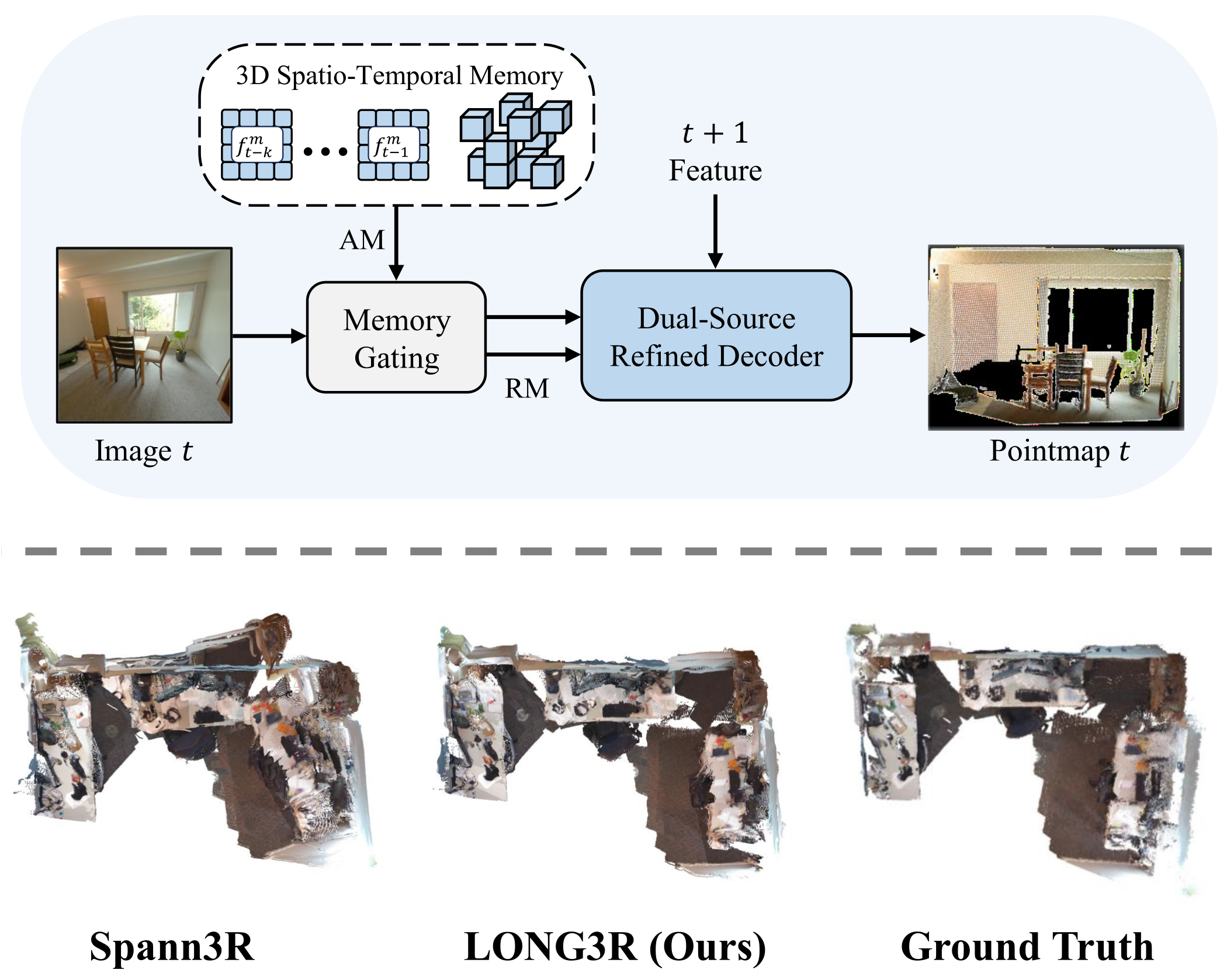
LONG3R reconstructs 3D pointmaps from image sequences using a recurrent network and bounded memory. Attention gating selects relevant history, a refined decoder alternates between that history and next-frame features, and voxel pruning limits spatial redundancy. Training progresses from five-frame to 10- and 32-frame sequences. At 224×224 resolution, it improves reconstruction over the tested streaming baselines on sequences of up to 200 sampled frames while running at roughly 21–22 frames per second on an RTX 3090. It still exhibits drift and viewpoint/dynamic-scene limitations.
1 Introduction
Pairwise pointmap models avoid much of the iterative geometry pipeline, but extending them to long sequences requires retaining useful context without accumulating redundant memory or errors. LONG3R builds on Spann3R’s recurrent reconstruction design [63] with selective memory access, repeated interaction with memory and adaptive 3D storage. “Long” means tens to hundreds of frames in this study, not indefinite error-free mapping.
The three proposed components are combined with a curriculum that expands training sequences. The decoder explicitly uses features from frame t+1 to predict frame t, so this streaming design includes one-frame look-ahead rather than strictly immediate prediction from present and past observations alone.
2 Related Work
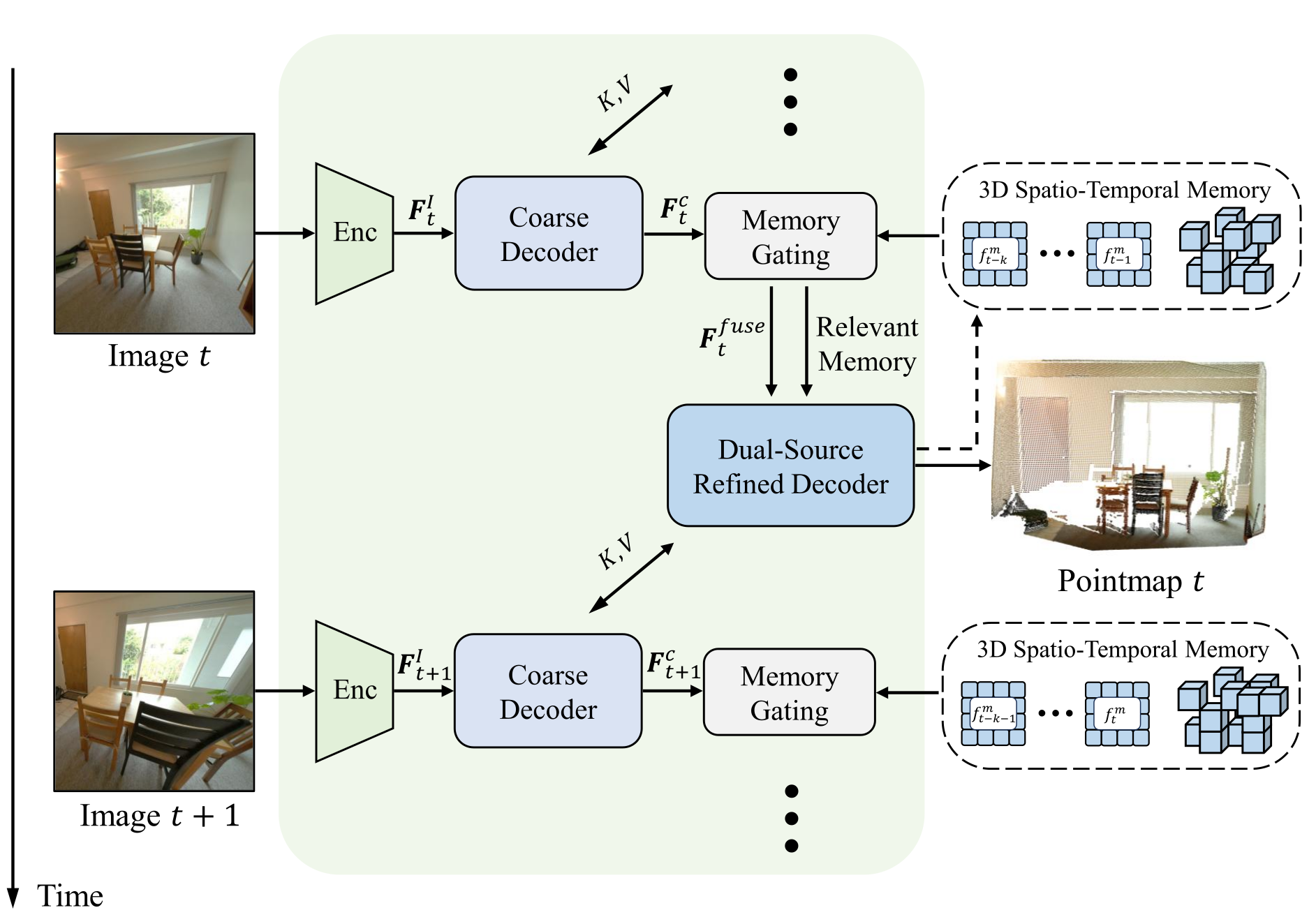
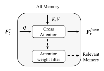
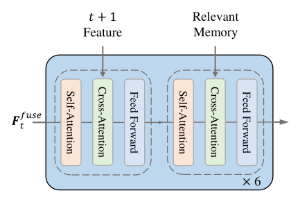
Figure 2 retains all three architecture panels, including the gating and alternating decoder blocks. The related work distinguishes geometric optimization, learned reconstruction and recurrent streaming models.
Traditional 3D Reconstruction.
Structure from motion and SLAM combine feature tracking, pose estimation and geometric optimization [49][61]. NeRFs and Gaussian splatting provide learned or optimized scene representations [37][27]. LONG3R instead regresses pointmaps using learned priors. This trades explicit global optimization for feedforward speed; it does not imply that every classical or optimized system requires the same calibration or has the same limitations.
Learning-Based 3D Reconstruction.
DUSt3R predicts geometry from image pairs, while MASt3R adds metric-scale geometry and matching [68][29]. Multi-view and recurrent models extend the representation to larger image sets [59][67]. LONG3R uses this pointmap foundation to improve how temporal and spatial history interact with each new view, rather than introducing a new renderer or globally optimized map representation.
Streaming Reconstruction.
Spann3R stores spatial features in memory, and CUT3R maintains a persistent recurrent state [63][67]. LONG3R reduces redundant spatial tokens and revisits relevant memory across decoder blocks. It has no explicit loop-closure or global post-optimization stage, so improved local/contextual consistency should not be confused with a guarantee against accumulated drift.
3 Method
Each frame is encoded and coarsely decoded, queries historical memory, and receives refined prediction using both relevant memory and the next frame. The pointmap supplies geometry for subsequent memory updates. All original mathematical definitions remain below.
3.1 Feature Encoding and Coarse Decoding
A Vision Transformer converts image patches into feature tokens. The coarse decoder applies self-attention, cross-attention and an MLP in each PairwiseBlock, interacting with the corresponding refined tokens from the preceding frame. Equation 2 specifies previous refined features; the architecture caption describes that input more loosely as previous image features.
Equations 1–2
| (1) |
| (2) |
3.2 Attention-based Memory Gating
Current coarse tokens attend to all stored keys and values, producing fused features and a P×S attention matrix. A memory token survives gating if any current patch assigns it attention above τ=5×10⁻⁴. The same mask selects keys and values for later refinement. This reduces downstream attention cost, but the initial gating operation still attends to the full memory bank. Relevance is measured by learned attention, not independently verified geometric usefulness.
Equations 3–6
| (3) |
| (4) |
| (5) |
| (6) |
3.3 Dual-Source Refined Decoder
Odd refined-decoder blocks interact with coarse tokens from frame t+1; even blocks attend to selected memory. A DPT prediction head converts the refined representation into a pointmap. Alternating sources is intended to avoid directly mixing mismatched feature spaces. That explanation is a design interpretation: the experiment compares decoder variants, without directly measuring feature-space alignment.
Equation 7
| (7) |
3.4 3D Spatio-Temporal Memory
Short-term memory stores patch keys and values from a recent time window. Long-term memory stores older features grouped by their predicted 3D positions. The experiments use ten recent frames and a 3,000-token long-term budget. These bounds concern feature memory, not storage of every predicted pointmap in the final accumulated reconstruction.
| Method | 7Scenes | NRGBD | FPS | ||||||||||
|---|---|---|---|---|---|---|---|---|---|---|---|---|---|
| Acc | Comp | NC | Acc | Comp | NC | ||||||||
| Mean | Med. | Mean | Med. | Mean | Med. | Mean | Med. | Mean | Med. | Mean | Med. | ||
| F-Recon [74] | 12.43 | 7.62 | 5.54 | 2.31 | 61.89 | 68.85 | 28.55 | 20.59 | 15.05 | 6.31 | 65.47 | 75.77 | 1 |
| Dust3R [68] | 3.01 | 1.47 | 5.11 | 2.79 | 58.83 | 63.73 | 3.94 | 2.48 | 5.31 | 3.58 | 62.62 | 72.29 | 3 |
| MASt3R [29] | 2.82 | 1.56 | 5.26 | 3.24 | 58.22 | 62.46 | 3.85 | 2.54 | 5.50 | 3.62 | 60.92 | 68.67 | 3 |
| MV-DUSt3R [59] | 2.92 | 1.24 | 2.49 | 0.78 | 66.42 | 76.07 | 3.76 | 1.99 | 2.55 | 0.92 | 81.16 | 95.39 | 15 |
| MV-DUSt3R+ [59] | 2.93 | 1.07 | 8.63 | 0.95 | 66.38 | 76.18 | 3.47 | 1.60 | 3.69 | 0.85 | 84.33 | 97.27 | 3 |
| CUT3R [67] | 7.73 | 3.57 | 7.75 | 1.83 | 65.74 | 73.98 | 12.48 | 5.57 | 6.34 | 2.35 | 75.84 | 90.05 | 23 |
| Spann3R[63] | 3.42 | 1.48 | 2.41 | 0.85 | 66.35 | 76.25 | 6.91 | 3.15 | 2.91 | 1.10 | 77.75 | 93.71 | 22 |
| Ours | 2.57 | 1.14 | 2.08 | 0.73 | 66.55 | 76.43 | 6.66 | 2.54 | 3.11 | 1.21 | 77.56 | 93.08 | 22 |
Adaptive Voxel Size.
A weighted average of predicted point coordinates gives each patch token a 3D location. Its local spacing is the mean Euclidean distance to eight neighboring image patches; this additional original formula is retained as a display. The smallest token spacing sets the image voxel size, and Equation 8 averages previous image voxel sizes to obtain the scene voxel size.
This adapts the discretization to relative scene scale without choosing a universal metric voxel width. Because spacing comes from predicted geometry and uses a minimum, it is not an independent geometric calibration. Initial-frame handling, boundary neighborhoods and the interaction between adaptive voxels and the hard capacity limit are not fully detailed in the paper.
Equations 8
| (8) |
3D Spatial Memory Pruning.
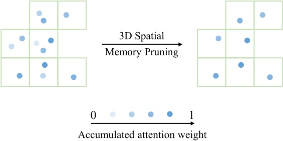
Tokens in the same voxel compete by accumulated attention, and only the highest-weight token is retained. Figure 3 preserves the before/after example. Pruning controls spatial redundancy, but discarded history can no longer be revisited through that token; the representation is an approximation to the observed scene.
| Method | Replica100 | Replica200 | FPS | ||||||||||
| Acc | Comp | NC | Acc | Comp | NC | ||||||||
| Mean | Med. | Mean | Med. | Mean | Med. | Mean | Med. | Mean | Med. | Mean | Med. | ||
| Dust3R [68] | 6.34 | 3.99 | 6.44 | 3.68 | 61.67 | 69.27 | 4.99 | 2.76 | 4.63 | 2.59 | 62.26 | 70.76 | 3 |
| MASt3R [29] | 5.10 | 2.96 | 6.00 | 3.43 | 61.81 | 69.52 | 5.26 | 3.23 | 7.31 | 3.75 | 58.03 | 62.81 | 3 |
| MV-DUSt3R [59] | 10.41 | 6.48 | 4.34 | 1.22 | 73.76 | 88.36 | 17.02 | 11.70 | 5.10 | 1.36 | 66.74 | 78.24 | 7 |
| MV-DUSt3R+ [59] | 5.28 | 3.26 | 2.56 | 0.89 | 79.07 | 93.63 | 11.79 | 8.37 | 5.64 | 1.53 | 70.66 | 83.86 | 1 |
| CUT3R [67] | 20.44 | 14.64 | 5.67 | 2.32 | 69.63 | 84.31 | 28.3 | 20.68 | 6.61 | 1.88 | 63.95 | 73.85 | 23 |
| Spann3R[63] | 14.08 | 8.88 | 4.67 | 1.61 | 72.46 | 88.98 | 16.29 | 10.17 | 4.02 | 1.16 | 68.56 | 82.80 | 21 |
| Ours | 11.46 | 7.55 | 3.68 | 1.24 | 73.29 | 89.86 | 11.93 | 7.42 | 2.73 | 0.87 | 68.67 | 82.92 | 21 |
3.5 Training
Training combines geometric regression with a sequence-length curriculum. The paper studies memory and decoder variants but does not report an isolated ablation of the entire curriculum.
Loss Function.
The total objective adds confidence-aware 3D regression and a scale penalty, following Spann3R and DUSt3R [63][68]. The scale term discourages predicted point clouds whose average distance exceeds the ground truth. Only the combined objective is written here; the complete definitions of its two inherited terms are referred to prior work. This objective does not establish globally consistent metric scale across arbitrary streams.
Equation 9
| (9) |
Two-stage Curriculum Training.
The first stage samples five frames per sequence and trains the network. The second freezes the ViT encoder and fine-tunes remaining modules first on ten-frame and then 32-frame sequences. The longer context encourages use of memory while reducing the cost of backpropagating through the encoder. Training length remains shorter than the 100/200-frame evaluation sequences.
4 Experiments
The evaluation covers dense reconstruction, camera pose and component ablations. The original tables preserve all mean/median metrics and speed columns, including cases where LONG3R is not best.
4.1 Setup
Training mixes six datasets; reconstruction evaluation uses three other datasets. Comparisons share the reported image resolution and evaluation GPU, but models still differ in architecture, pretrained weights, optimization and training exposure.
Training Datasets.
The mixture is Habitat, ARKitScenes, BlendedMVS, ScanNet++, Co3D-v2 and ScanNet [48][4][80][82][45][10]. It includes real and synthetic examples with metric and normalized scales. Training scenes are static, which limits conclusions about large moving objects.
Baselines.
Spann3R and CUT3R are the main streaming baselines. DUSt3R and MASt3R include post-processing, while MV-DUSt3R and its plus variant operate offline. All listed tests use 224×224 images on one 24GB RTX 3090. This makes the reported timing setting concrete without equating offline throughput, streaming latency and all end-to-end application costs.
Implementation details.
The encoder is ViT-Large initialized from DUSt3R [14][68]. Stage one uses AdamW, learning rate 1.12×10⁻⁴, batch ten per GPU and 120 epochs. Stage two uses learning rate 10⁻⁵ for twelve epochs each at ten and 32 views. Training takes about 28 plus 20 hours on sixteen A100s, approximately 768 GPU-hours, excluding DUSt3R pretraining. Repeated-seed confidence intervals are not reported.
| Method | 7Scenes | TUM | ScanNet | ||||||
|---|---|---|---|---|---|---|---|---|---|
| ATE | RPEt | RPEr | ATE | RPEt | RPEr | ATE | RPEt | RPEr | |
| Spann3R [63] | 12.64 | 6.15 | 1.88 | 5.66 | 2.13 | 0.59 | 9.83 | 2.30 | 0.66 |
| CUT3R [67] | 12.40 | 7.65 | 2.34 | 6.25 | 2.55 | 0.69 | 14.27 | 3.58 | 0.92 |
| Ours | 8.72 | 5.03 | 1.67 | 5.40 | 2.36 | 0.60 | 6.44 | 2.14 | 0.61 |
4.2 3D Reconstruction
Reconstruction is evaluated on 7Scenes, NRGBD and Replica with accuracy, completion and normal consistency [52][3][54]. Lower distance errors in centimeters and higher normal consistency are better. Replica samples 100 or 200 observations from the same scene; this changes observation density and processed frame count, not necessarily the physical path length or duration.
Quantitative comparisons.
On 7Scenes, LONG3R’s mean accuracy/completion are 2.57/2.08cm, compared with Spann3R’s 3.42/2.41cm and CUT3R’s 7.73/7.75cm, at approximately 22 FPS. On NRGBD, its mean accuracy 6.66cm improves on Spann3R’s 6.91cm, but completion 3.11cm is worse than 2.91cm and normal consistency is also slightly lower. Improvement is therefore not uniform across metrics.
On Replica, LONG3R’s mean accuracy changes from 11.46cm at 100 frames to 11.93cm at 200, whereas Spann3R worsens from 14.08 to 16.29cm and CUT3R from 20.44 to 28.30cm. LONG3R runs at roughly 21 FPS. At 200 frames, MASt3R’s mean accuracy is much better at 5.26cm, but its reported speed is at most 3 FPS. The result supports a speed/quality trade-off among these settings rather than elimination of drift or dominance over optimized methods.
| Method | 7Scenes | NRGBD | FPS | ||||||
| Acc | Comp | Acc | Comp | ||||||
| Mean | Med. | Mean | Med. | Mean | Med. | Mean | Med. | ||
| w/o Gating | 2.53 | 1.12 | 2.12 | 0.74 | 6.72 | 3.14 | 2.91 | 1.20 | 18.0 |
| w/ Gating | 2.57 | 1.14 | 2.08 | 0.73 | 6.66 | 3.11 | 2.92 | 1.21 | 21.4 |
Qualitative comparisons.
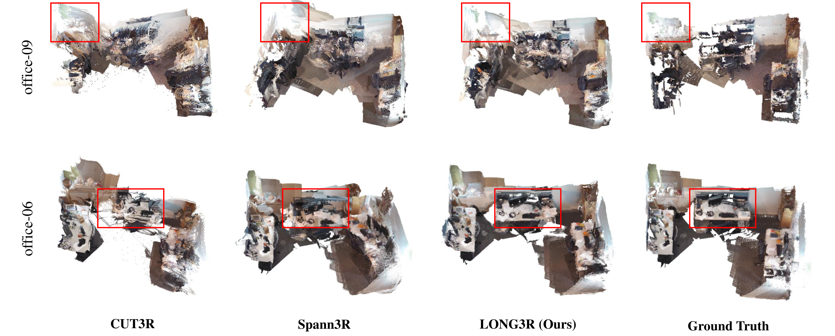
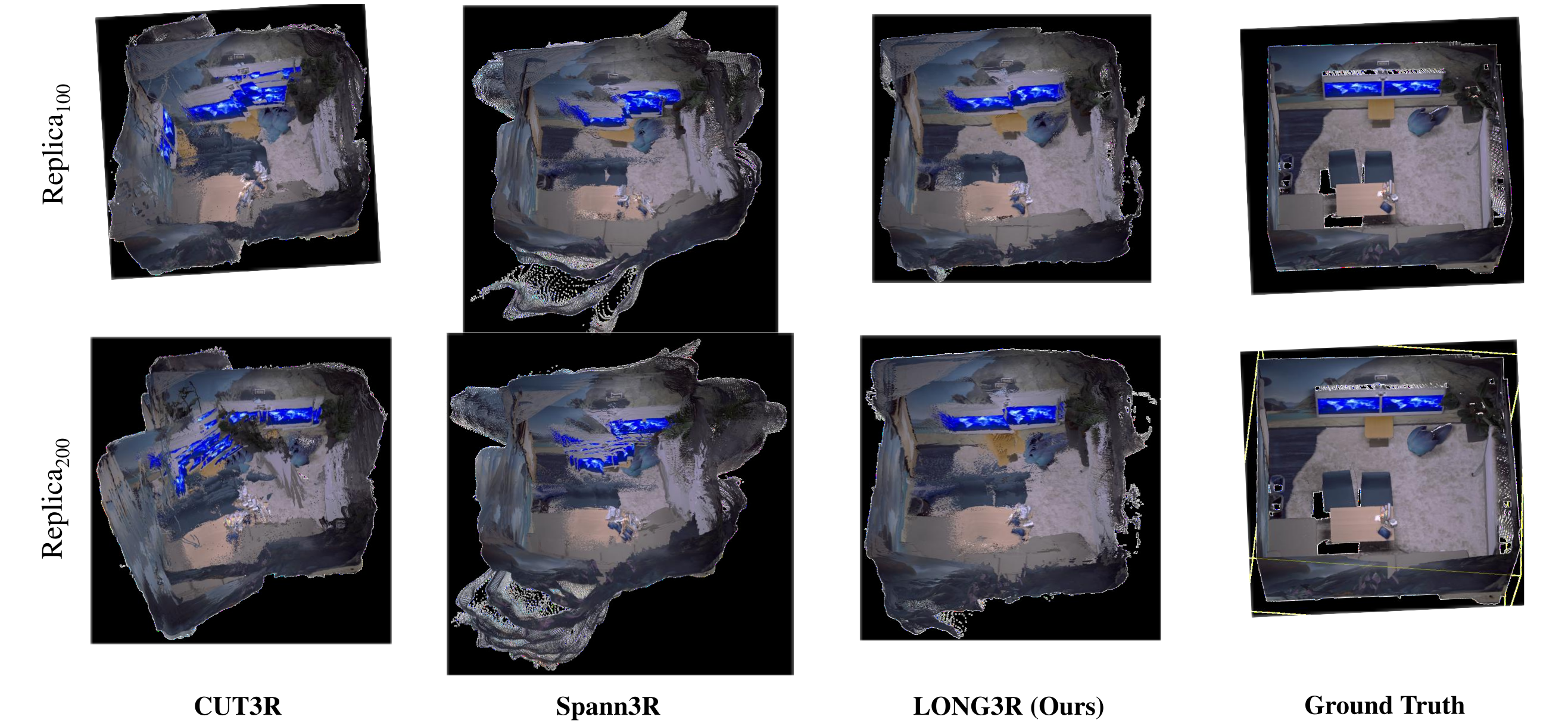
Figures 4–5 preserve both office scenes and both Replica sampling densities for CUT3R, Spann3R, LONG3R and ground truth. Highlighted regions show selected reductions in duplicated or distorted surfaces. These qualitative examples complement aggregate metrics; they do not demonstrate every viewpoint, dynamic scene or revisitation pattern.
4.3 Camera Pose Estimation
Pose errors are reported as absolute translation error and relative translation/rotation errors, with translation in centimeters and rotation in degrees. LONG3R improves all three listed measures on 7Scenes and ScanNet: ATE is 8.72cm and 6.44cm, respectively. ScanNet is also one of the training dataset sources, so it is not evidence of an entirely unseen dataset distribution.
TUM Dynamics is mixed: LONG3R’s ATE 5.40cm improves on Spann3R’s 5.66cm and CUT3R’s 6.25cm, while its relative translation/rotation errors 2.36cm/0.60° trail Spann3R’s 2.13cm/0.59°. Static-only training can still produce competitive results on these sequences, but does not establish robust handling of large object motion.
4.4 Ablation and analysis
The ablations separately compare memory gating, interleaved decoding and spatial-memory designs. Their configurations differ where explicitly noted, so their numerical results should not all be treated as the main model’s identical training run.
Attention-based Memory Gating.
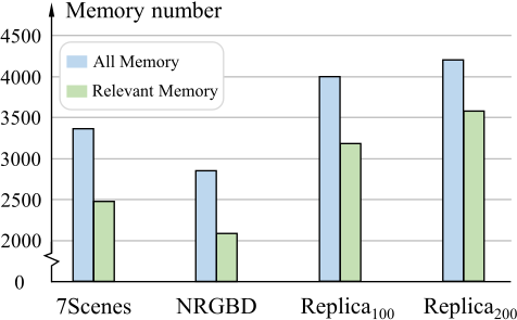
Gating removes about 27% of stored tokens from the refinement attention on 7Scenes and raises throughput from 18.0 to 21.4 FPS, an 18.9% increase, rounded to 20% in the paper. Accuracy changes are mixed: 7Scenes mean accuracy slightly worsens from 2.53 to 2.57cm while completion improves from 2.12 to 2.08cm. Table 4’s NRGBD median accuracy and mean completion differ from Table 1’s main-model values; the source does not explain that discrepancy.
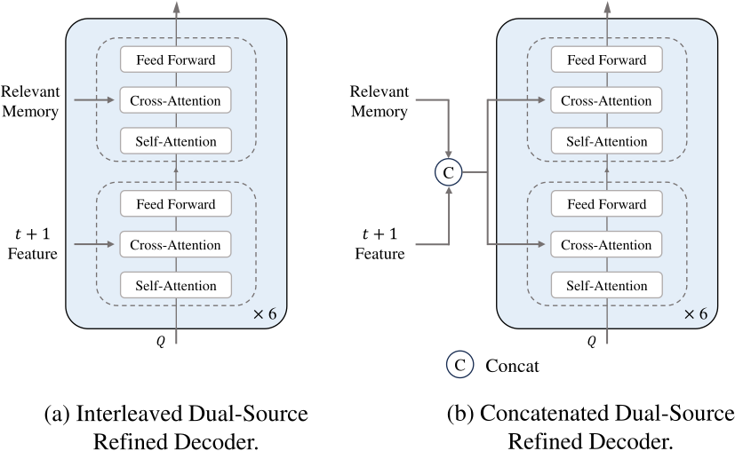
Dual-Source Refined Decoder.
The decoder comparison uses 24-frame fine-tuning because concatenation exceeds the stated memory constraints at 32 frames. At 200 evaluation frames, interleaving improves mean accuracy from 29.52 to 13.34cm and completion from 8.88 to 3.15cm. Figure 7 retains both architectures. These results support the interleaved design under a matched 24-frame comparison, not the same numerical setting as the main 32-frame model.
3D Spatio-Temporal Memory.
Without long-term spatial memory, Replica-200 mean accuracy degrades to 65.75cm, versus 11.93cm for the full design. Replacing it with Spann3R memory under the same network gives 12.41cm, a much smaller difference. Thus the major demonstrated effect is retaining long-term context; adaptive spatial pruning provides an additional gain in the reported comparison.
| Method | Replica100 | Replica200 | ||||||
|---|---|---|---|---|---|---|---|---|
| Acc | Comp | Acc | Comp | |||||
| Mean | Med. | Mean | Med. | Mean | Med. | Mean | Med. | |
| Concat. | 14.83 | 10.26 | 4.59 | 1.81 | 29.52 | 21.04 | 8.88 | 4.05 |
| Interleaved. | 12.06 | 7.67 | 3.68 | 1.23 | 13.34 | 8.41 | 3.15 | 0.94 |
| Method | 7Scenes | Replica200 | ||||||
|---|---|---|---|---|---|---|---|---|
| Acc | Comp | Acc | Comp | |||||
| Mean | Med. | Mean | Med. | Mean | Med. | Mean | Med. | |
| w/o 3D Spa. Mem. | 5.76 | 2.96 | 3.30 | 1.22 | 65.75 | 47.63 | 13.24 | 3.49 |
| w/ Spann3R Mem. | 2.64 | 1.16 | 2.10 | 0.74 | 12.41 | 7.87 | 3.07 | 0.88 |
| LONG3R (ours) | 2.57 | 1.14 | 2.08 | 0.73 | 11.93 | 7.42 | 2.74 | 0.87 |
5 Conclusion
LONG3R improves the efficiency and consistency of recurrent pointmap reconstruction through selective memory access, alternating attention and spatial pruning. It remains anchored to the first frame and can blur when viewpoints diverge substantially. Large object motions are difficult because training is static. The experiments do not establish unlimited operation, drift-free global mapping, broad outdoor transfer, or performance at higher image resolutions; those remain beyond the measured scope.
Acknowledgements
The authors acknowledge support from China’s National Key R&D Program (2022ZD0161700) and Tsinghua University’s Initiative Scientific Research Program.