At a glance
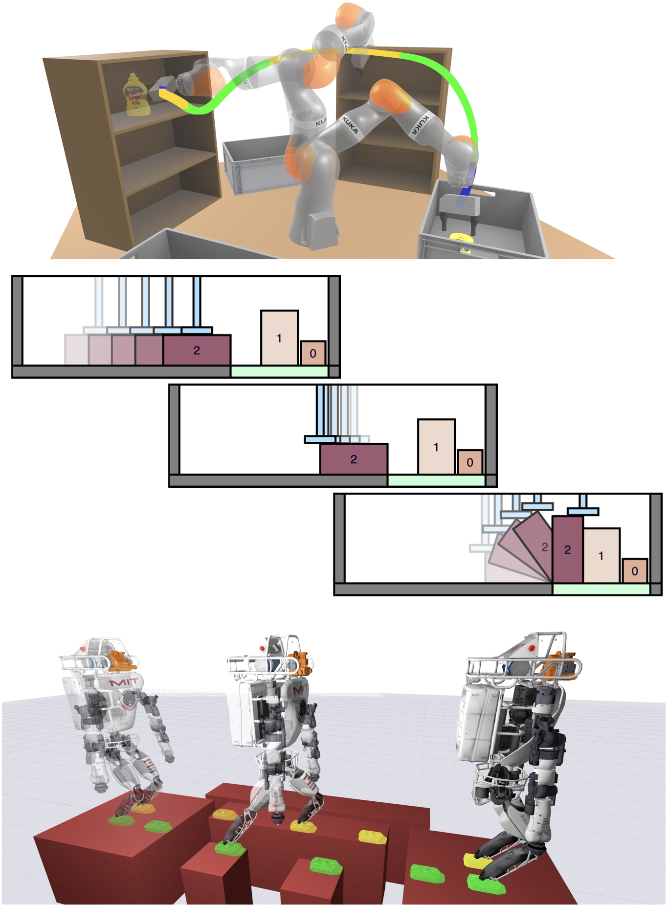
A graph of convex sets couples discrete mode choices with continuous optimization. Unlike a path, a walk may revisit a mode at a different continuous state, making repeated actions and variable-duration behavior natural to express. The paper builds quadratic lower bounds on remaining cost with semidefinite programming, then uses them to guide a fast approximate search.
Demonstrations cover acceleration-limited arm motion, rearrangement skills and simplified bipedal planning. Reported query speeds exclude substantial reusable preparation and use simulated parallel solver timing; the practical greedy search is neither complete nor globally optimal.
I Introduction
In an ordinary nonnegative-cost graph, deleting a cycle cannot worsen the route. In a graph of convex sets, revisiting the same vertex can select a new continuous point and make useful progress. This makes shortest walks materially different from shortest paths.
The method extends cost-to-go-guided GCS search: synthesize one convex quadratic lower bound per vertex, then choose successive transitions using those bounds. The formulation is general, while the numerical method imposes convex/quadratic structure and trades guarantees for speed.
II Shortest Walks in Graphs of Convex Sets
A solution chooses the number of steps, the sequence of discrete vertices and a feasible continuous trajectory through them. Repetition is allowed and can improve cost.
II-A Preliminaries
Vertices carry local convex optimization problems; edges specify which consecutive continuous decisions can coexist.
Graph of Convex Sets (GCS)
Each vertex has a compact convex feasible set and a nonnegative convex cost. Each directed edge has a convex coupling set contained in the product of its endpoint sets, plus a nonnegative convex transition cost. Visiting a vertex selects a point in its set; crossing an edge must satisfy its coupling constraint.
Walk in a GCS
A K-step walk contains K+1 vertex visits and continuous points, with fixed source/target points and feasible consecutive edges. Repeated visits may select different continuous points. Total cost sums every visited vertex cost and every transition cost, including repeated visits.
Equations 1a–1d
| (1a) | |||||
| (1b) | |||||
| (1c) | |||||
| (1d) | |||||
II-B Shortest-walk problem
The inner optimization finds the best feasible discrete/continuous walk of a fixed length; the outer infimum ranges over all lengths. This avoids choosing a fixed horizon in the problem definition, although the search implementation uses finite lookahead.
Equations 2a–2b
| (2a) | ||||
| (2b) | ||||
II-C Shortest walks need not be paths
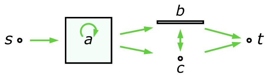
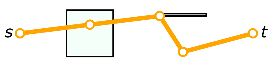
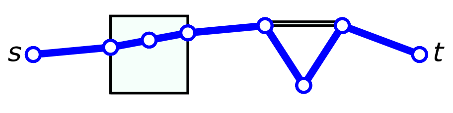
Figure 2 provides a counterexample to removing cycles: each edge costs one plus squared displacement. Revisiting vertices permits smaller, cheaper movements. The best illustrated walk costs 28, while the best path costs 35. Repetition changes the continuous state, so it is not wasted travel.
II-D Sufficient condition for finiteness of shortest walks
Without a strictly positive per-step charge, infinitely many smaller steps can approach an infimum that no finite walk attains. A positive minimum cost on every edge is a sufficient condition excluding an infinite-length finite-cost optimum. Adding epsilon to each edge enforces it but also changes the planning objective. The discussion assumes a feasible optimum exists.
Equation
III Applications in robotics and control
Walks are useful when repeated local trajectories, skills or hybrid modes are necessary. Paths remain appropriate when repetition is forbidden or unnecessary.
III-A Collision-free motion planning with acceleration limits
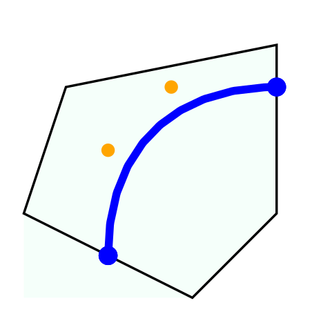
Standard GCS motion planning assigns a collision-free convex region to each vertex and a Bézier segment to each visit. Jointly optimizing segment shape and duration makes acceleration constraints nonconvex, motivating time rescaling or local nonlinear post-processing.
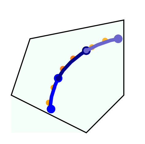
Fixing each segment’s duration makes derivative constraints convex. A walk can spend more time in a region by revisiting it, without duplicating vertices. This gives a compact formulation, but does not eliminate time discretization: very small fixed durations can create long walks. Region construction is a separate prerequisite.
III-B Skill chaining
Represent a skill by the set of feasible start/end configurations and a transition cost. A vertex visit executes one skill; edge constraints equate the preceding end configuration with the following start. Source and target vertices impose the task endpoints.
The shortest walk then jointly selects a skill sequence and continuous transition parameters. Exact equivalence requires convex skill transition sets and costs; otherwise convex approximations or decompositions must be supplied, potentially with considerable manual effort.
III-C Optimal control for hybrid systems
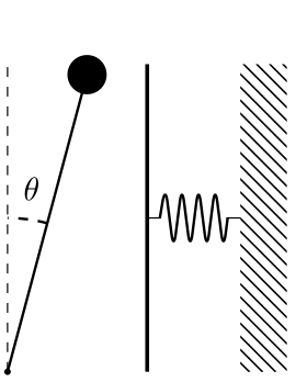
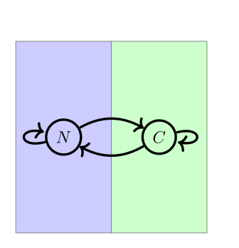
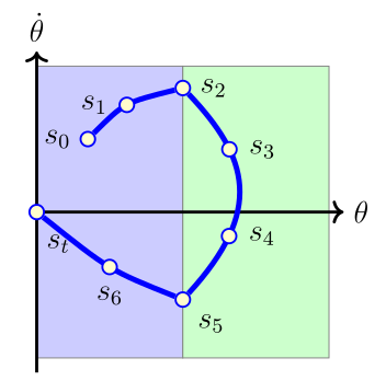
For a piecewise-affine system, create a vertex for each mode’s state/control set and impose its affine dynamics as edge constraints. Vertex costs are stage costs; revisiting a mode corresponds to spending additional time there or returning later. The soft-wall pendulum illustrates two contact modes.
The construction applies directly to the stated convex piecewise-affine model. Approximating nonlinear or contact-rich physics is an additional modeling step, not a guarantee that the resulting plan remains exact for the original system.
Equation
IV Solution method
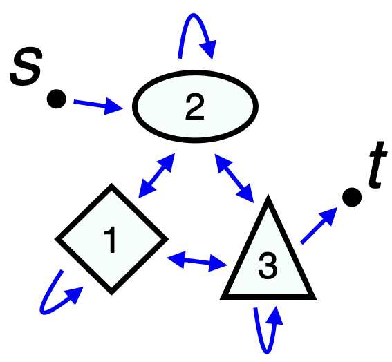
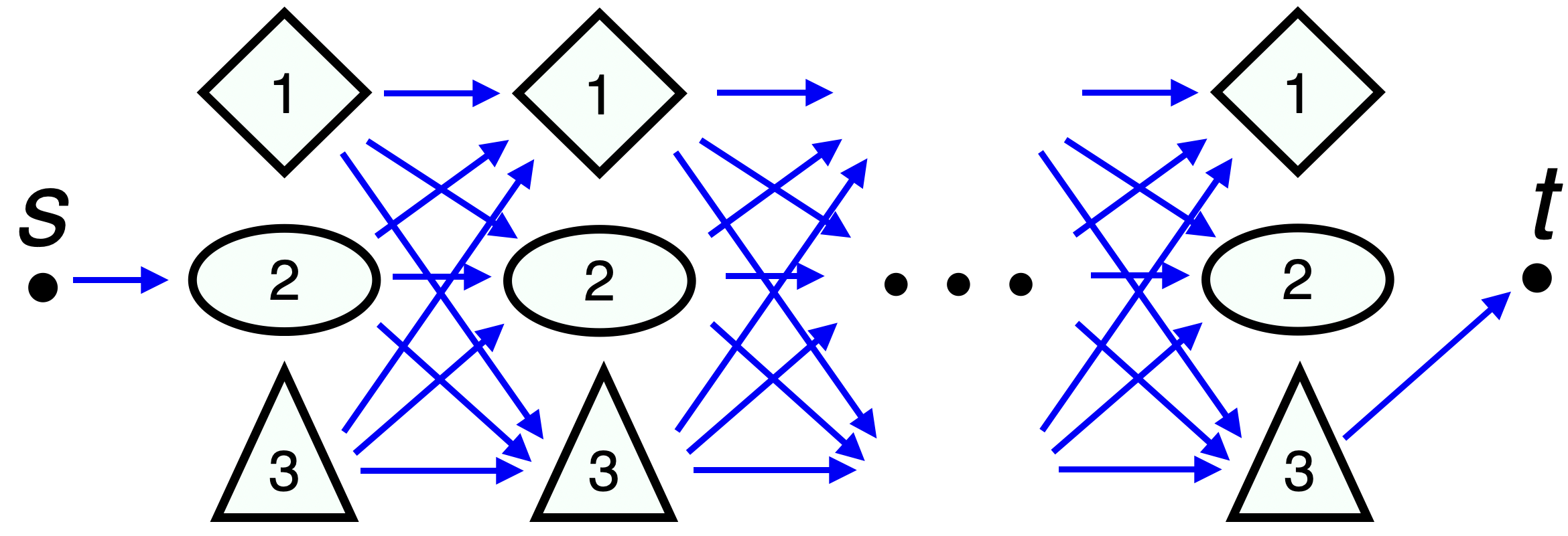
Shortest walks remain NP-hard: on an acyclic graph they coincide with the already-hard shortest-path problem. Increasing-horizon layered copies provide a conceptual solution but enlarge the optimization repeatedly.
The proposed alternative works on the original graph. It synthesizes lower bounds through Bellman inequalities, then uses those bounds as a search heuristic. The bound representation scales with graph size rather than an explicitly unrolled horizon, although query complexity still depends on branching and walk length.
IV-A Bellman equation
An optimal walk has optimal subwalks. Its cost-to-go equals the current vertex cost plus the best feasible edge cost and successor cost-to-go, minimizing over both the next discrete vertex and continuous point. The successor may be the same vertex.
Equation 3
| (3) | ||||
IV-B Synthesis of cost-to-go lower bounds
Replace Bellman equality with an inequality and fix the target value to its terminal vertex cost. Any feasible family of functions lower-bounds the optimal remaining cost. Maximizing the source value gives the exact source cost in the unrestricted infinite-dimensional formulation.
Objectives averaged over vertices/states, or extended to target states, support reusable bounds for multiple queries. The practical finite-dimensional approximation retains a lower-bound interpretation but generally loses tightness.
Equations 4a–4d
| (4a) | ||||
| s.t. | (4b) | |||
| (4c) | ||||
| (4d) | ||||
IV-C Tractable finite-dimensional cost-to-go lower bounds
The numerical method restricts per-vertex bounds to convex quadratics, feasible sets to polyhedra/ellipsoid intersections and costs to convex quadratics or suitable approximations. Semidefinite constraints provide tractable nonnegativity certificates. Higher-degree sums-of-squares relaxations could be more expressive but cost more.
Bound synthesis is the expensive preparation stage, often seconds to over a minute. Reuse in a fixed environment can amortize that cost; the query-time results alone do not describe initial planning latency.
IV-D Extracting walks from the approximate cost-to-go
At each step, enumerate finite-horizon candidate walks, solve their continuous convex programs in parallel and select the best accumulated cost plus terminal lower bound. The final vertex cost is subtracted once to avoid double counting. Commit only the first transition and repeat, allowing early arrival at the target.
An infeasible step triggers backtracking, and a fixed iteration budget can terminate the search. These choices give no completeness or optimality guarantee. Afterward, reoptimize all continuous points along the selected walk and remove cycles only when reoptimization preserves feasibility and lowers cost.
Equations 5a–5c
| (5a) | ||||
| s.t. | (5b) | |||
| (5c) | ||||
V Results
Experiments use Mosek for convex programs and SNOPT for the nonlinear baseline on an Apple M1 Max laptop with 16 GB RAM. The paper reports simulated parallelized solver times, assuming up to ten solves in parallel and prebuilt program binaries; these are not straightforward measured end-to-end wall-clock times.
V-A Collision-free motion planning with acceleration limits
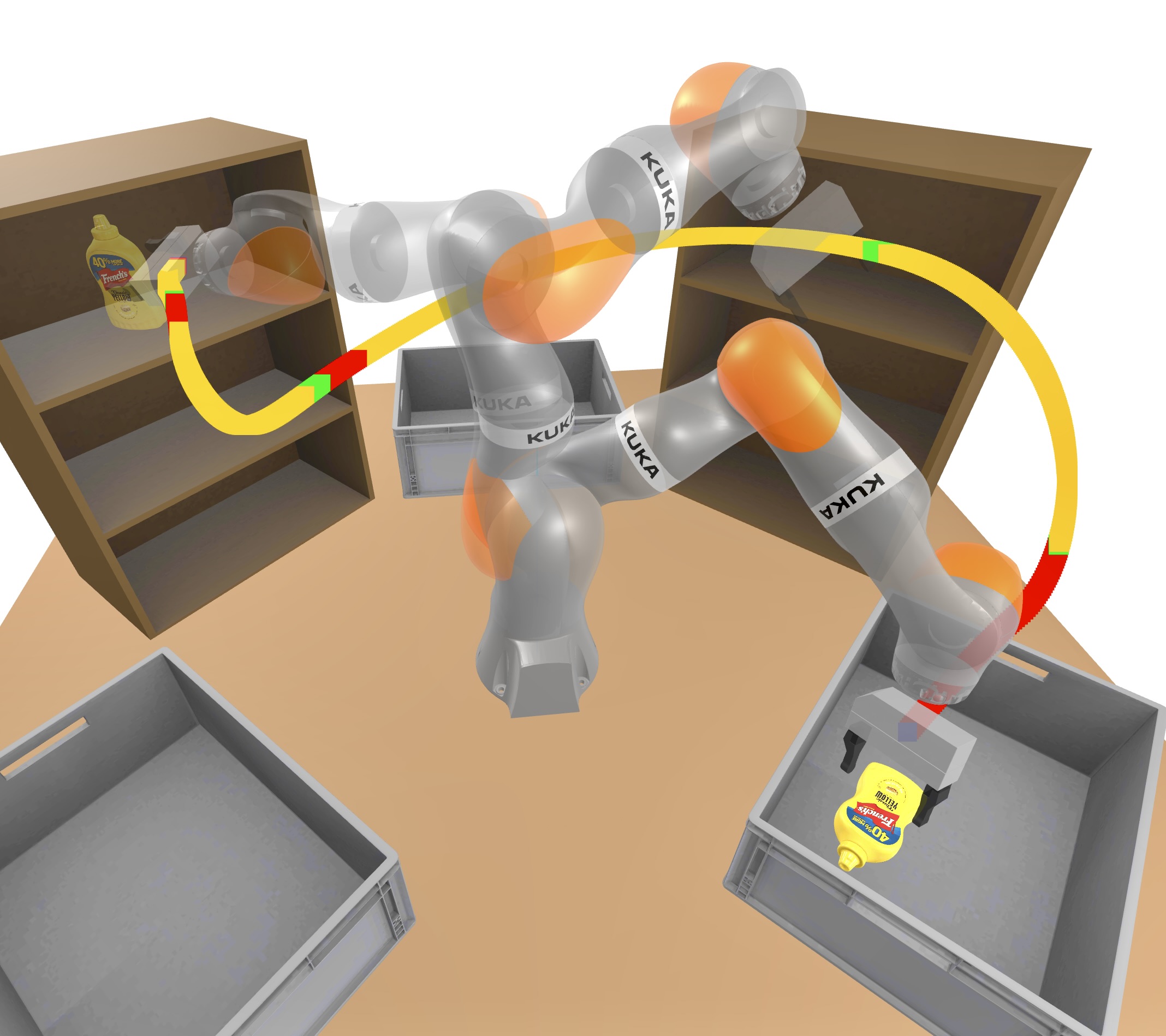
Warehouse arm planning uses 16 convex regions and 54 edges. Region decomposition costs 100 seconds and reusable lower-bound synthesis another 45 seconds. Each walk visit uses a 125 ms cubic Bézier segment, enforcing acceleration limits during search.
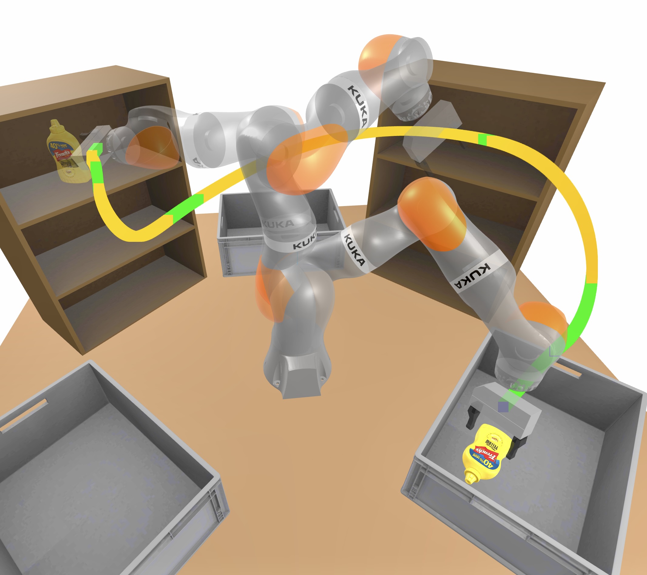
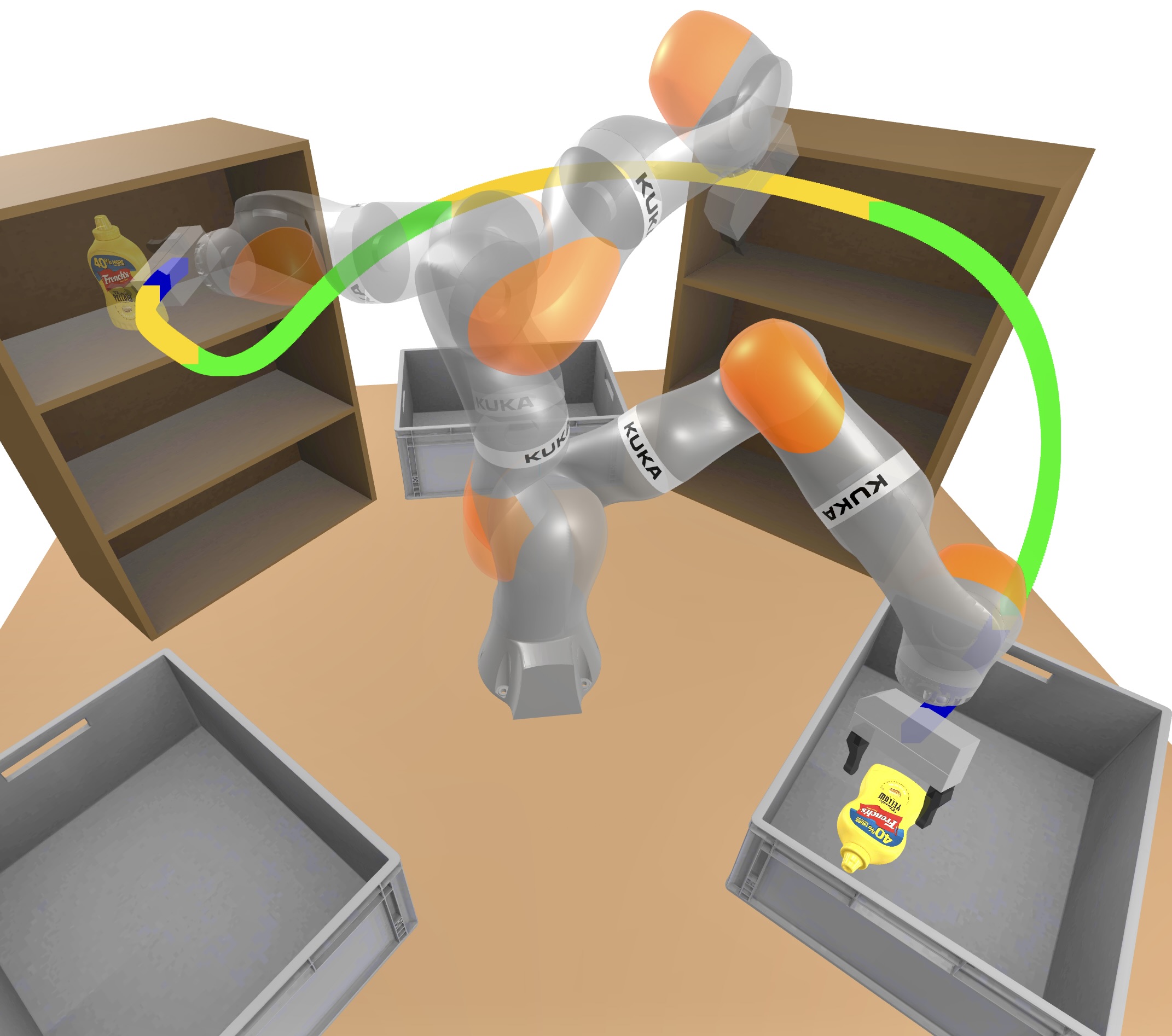
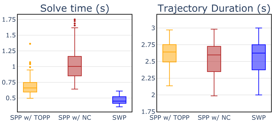
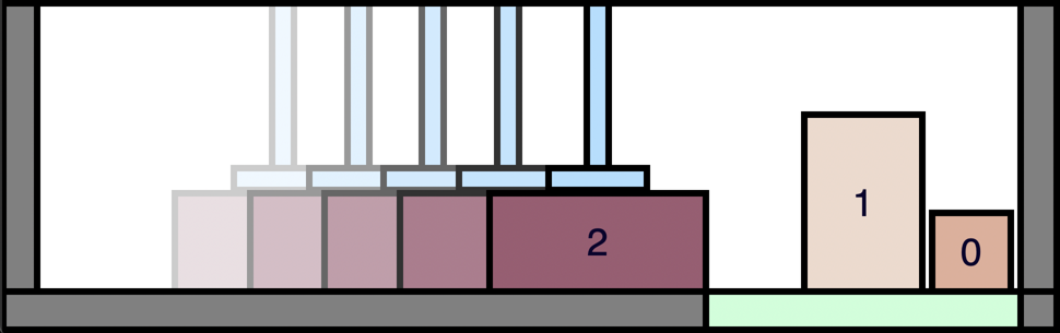
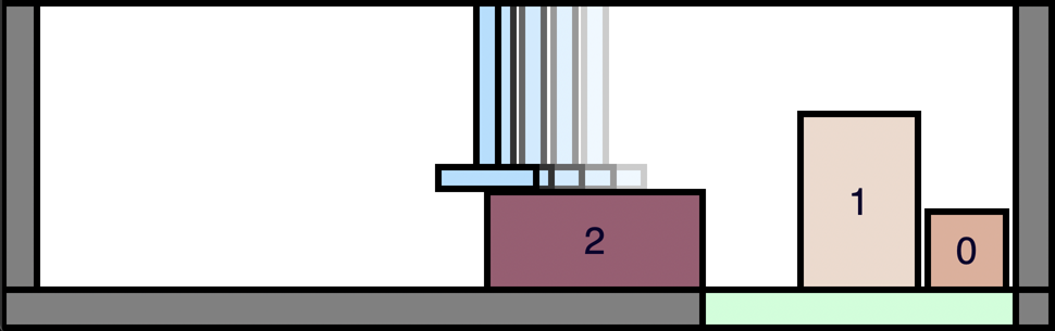
Across 100 queries, reported average query time is 0.46 seconds: 1.5× faster than shortest paths with time-optimal path parameterization and 2.3× faster than the nonlinear post-processing baseline. Average trajectory durations differ by only 1–2%. In the pictured example, the walk takes 2.25 seconds versus 2.57 seconds after rescaling the path; the original 2.21-second path violates acceleration limits.
Higher derivative constraints can also fit the fixed-duration formulation, but jerk-limited performance is not separately evaluated. The displayed studies use virtual items and do not establish real-hardware execution reliability.
V-B Skill chaining
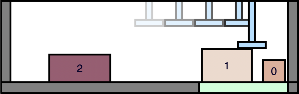
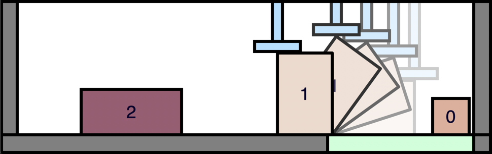
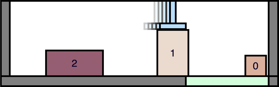
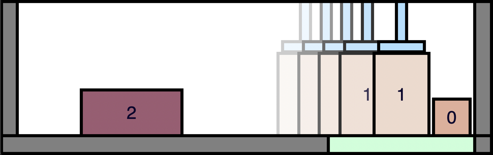
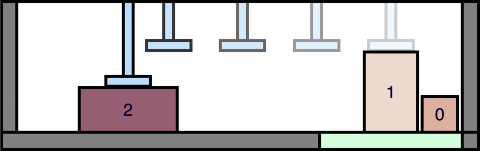
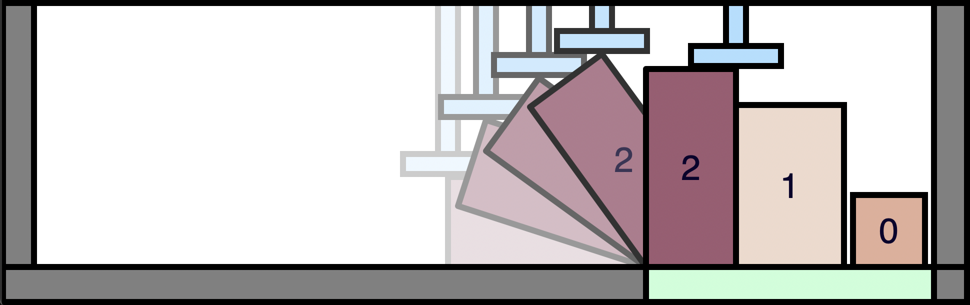
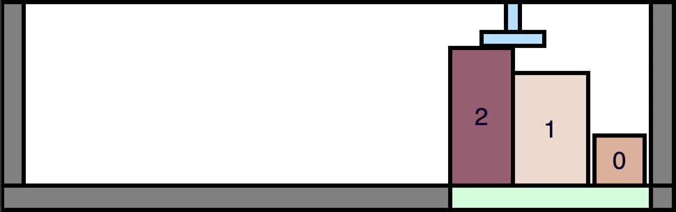
A simplified suction gripper moves horizontally and rearranges three rectangular objects using movement, centered pick/place and corner-flipping skills. Convex decomposition yields 15 subskills plus endpoint vertices, giving 22 vertices and 120 edges. Each skill costs one plus arm displacement.
Bound synthesis takes 20 seconds; reported query times are 0.5–1 second with prebuilt programs. The illustrated eight-action plan temporarily moves an already-placed object to fit another. The claim that sampling methods would struggle is qualitative; no timed sampling baseline is provided. The text calls this example optimal without establishing a general optimality guarantee for its greedy solver.
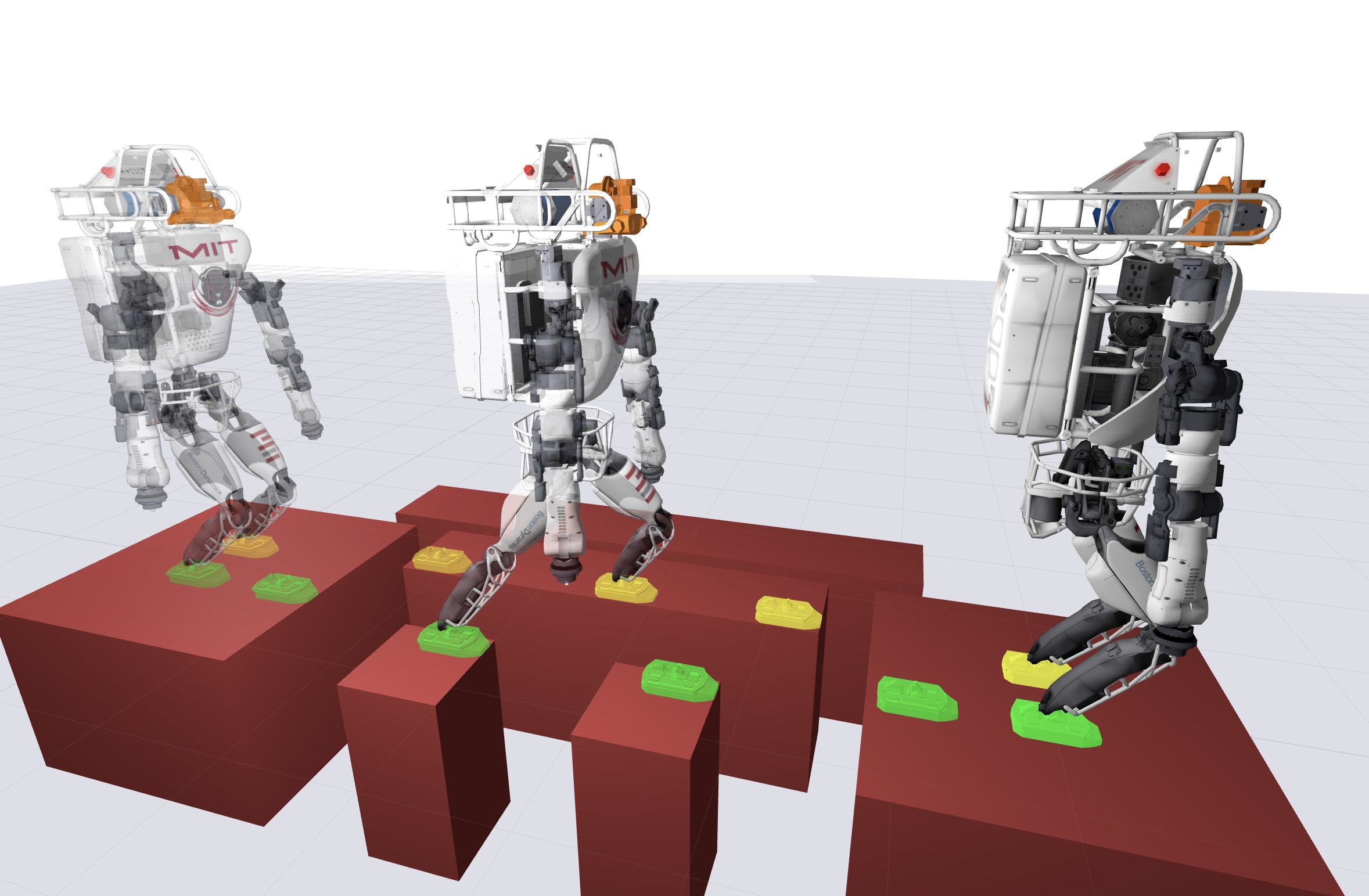
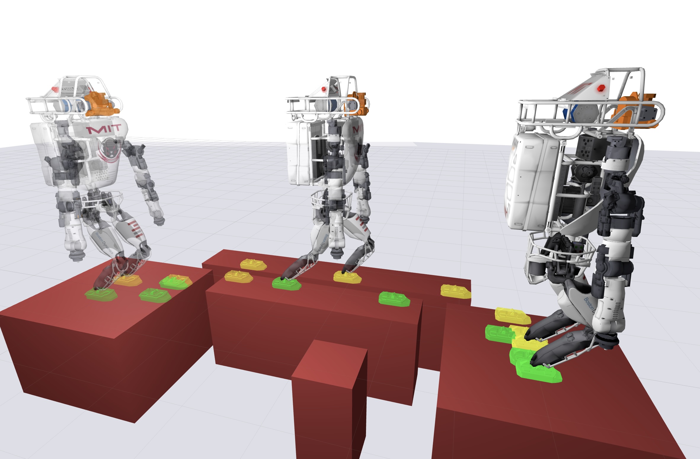
V-C Hybrid dynamics: footstep planning for a ZMP walker
The bipedal example uses a zero-moment-point model with zero vertical acceleration, zero angular acceleration and fixed foot orientation. Friction, support-polygon and foot-collision constraints define piecewise-affine contact modes; this is a simplified model, not full humanoid dynamics.
Two layouts produce graphs with 24 vertices/58 edges and 21 vertices/50 edges. Lower-bound synthesis takes 2.3 and 3.7 seconds; reported searches produce 10- and 16-step plans in 110 and 330 ms. Receding-horizon disturbance rejection is suggested, but not demonstrated by a disturbance experiment.
VI Limitations
Building convex collision regions, decomposing skills and constructing piecewise-affine dynamics can be costly and require manual tuning. Large semidefinite programs limit online use unless their bounds can be reused. Fast search depends on prebuilding and parallelization, and the reported parallel timing is simulated.
The work’s main contribution is a compact modeling language for repeated modes plus a useful heuristic. It does not remove NP-hardness, convex-modeling assumptions, finite-duration discretization or the practical search’s lack of completeness and global optimality.