Overview
The supplementary material documents contributors, hardware and simulation platforms, task data, initial conditions, scoring rubrics, missing trials, failure analysis, data filtering, and the normalization-error follow-up. These details materially qualify the main performance claims.
At a glance
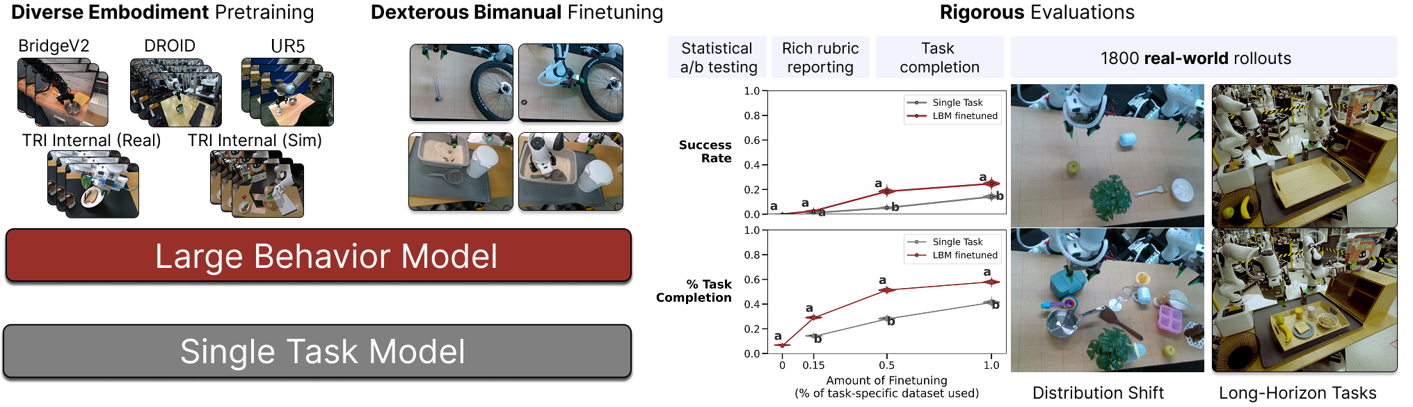
Using a fixed diffusion-transformer architecture, the study tests whether broad robot-data pretraining improves task-specific manipulation policies. Across controlled simulation and blinded physical trials, fine-tuned specialists generally learn with fewer demonstrations, achieve higher aggregate performance, and better withstand the tested distribution shifts than single-task baselines. Unadapted multitask policies are less consistently competitive. The contribution is a carefully measured pretraining comparison and evaluation protocol rather than a new architecture.
1 Introduction
The question is whether multitask robot pretraining provides a measurable advantage over task-specific behavior cloning. Models use roughly 1,700 hours of heterogeneous demonstrations, and the main study reports 1,800 controlled physical trials plus extensive simulation. The strongest findings concern fine-tuned specialists: less target-task data, better aggregate outcomes, and greater robustness under selected shifts. These claims do not imply reliable zero-shot execution of arbitrary new tasks.
2 Related Work
The study connects large-scale policy training, the cost and heterogeneity of robot demonstrations, and the need for reproducible manipulation evaluation.
2.1 Robot Learning at Scale
Prior robot foundation models vary in backbone, action representation, training data, and transfer from language or vision. To reduce these confounds, this study fixes its policy architecture while changing robot pretraining and task-specific adaptation. It does not compare all contemporary architectures or establish a model-size scaling law.
2.2 Datasets for Robot Learning
Teleoperation provides embodied supervision but is expensive to scale. The training mixture combines internal robot demonstrations, handheld manipulation recordings, public cross-embodiment datasets, and simulation. Real/simulation co-training also makes simulation evaluation of largely real-data-trained policies feasible, without assuming exact transfer between the two domains.
2.3 Evaluating Robotic Manipulation Policies
Simulators offer repeatability and throughput, while physical benchmarks face hardware variation and sensitivity to small scene changes. Success rates alone can hide partial progress or failure modes. The paper emphasizes controlled resets, sufficient trial counts, explicit milestones, and analysis of deployment shifts.
Related source: best practices for policy evaluation.
3 Results
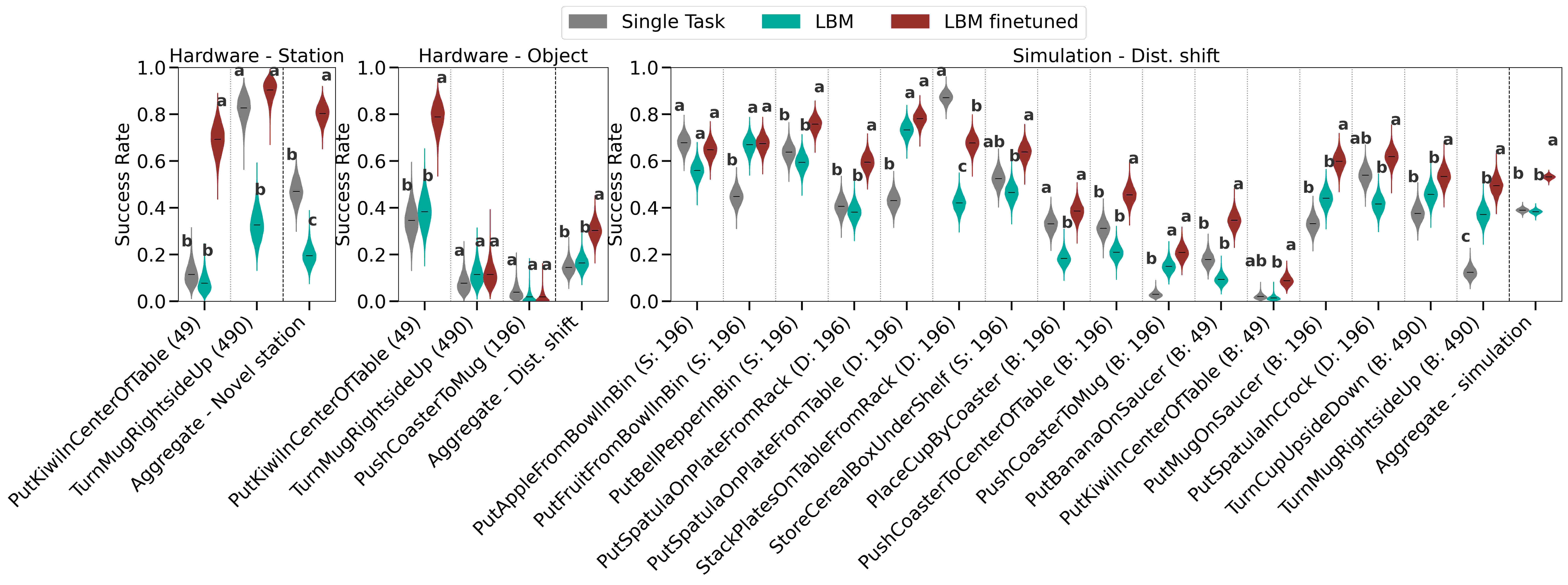
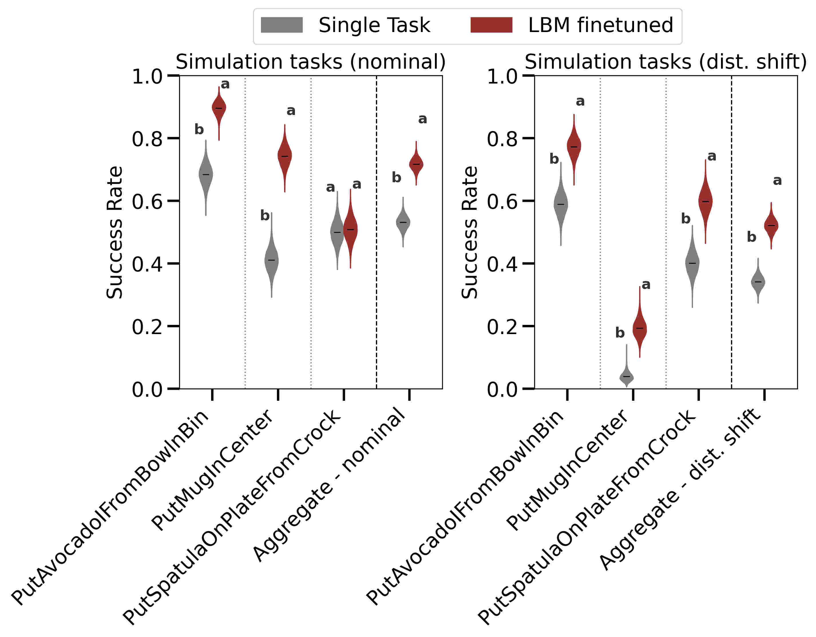
Evaluation distinguishes tasks present in robot pretraining from held-out tasks, and nominal conditions from deliberate shifts. The target is 50 hardware or 200 simulation rollouts per policy/task/condition. Success measures final completion; task-completion scores measure achieved milestones. The authors deliberately choose challenging settings, so absolute rates depend strongly on task design and demonstration coverage.
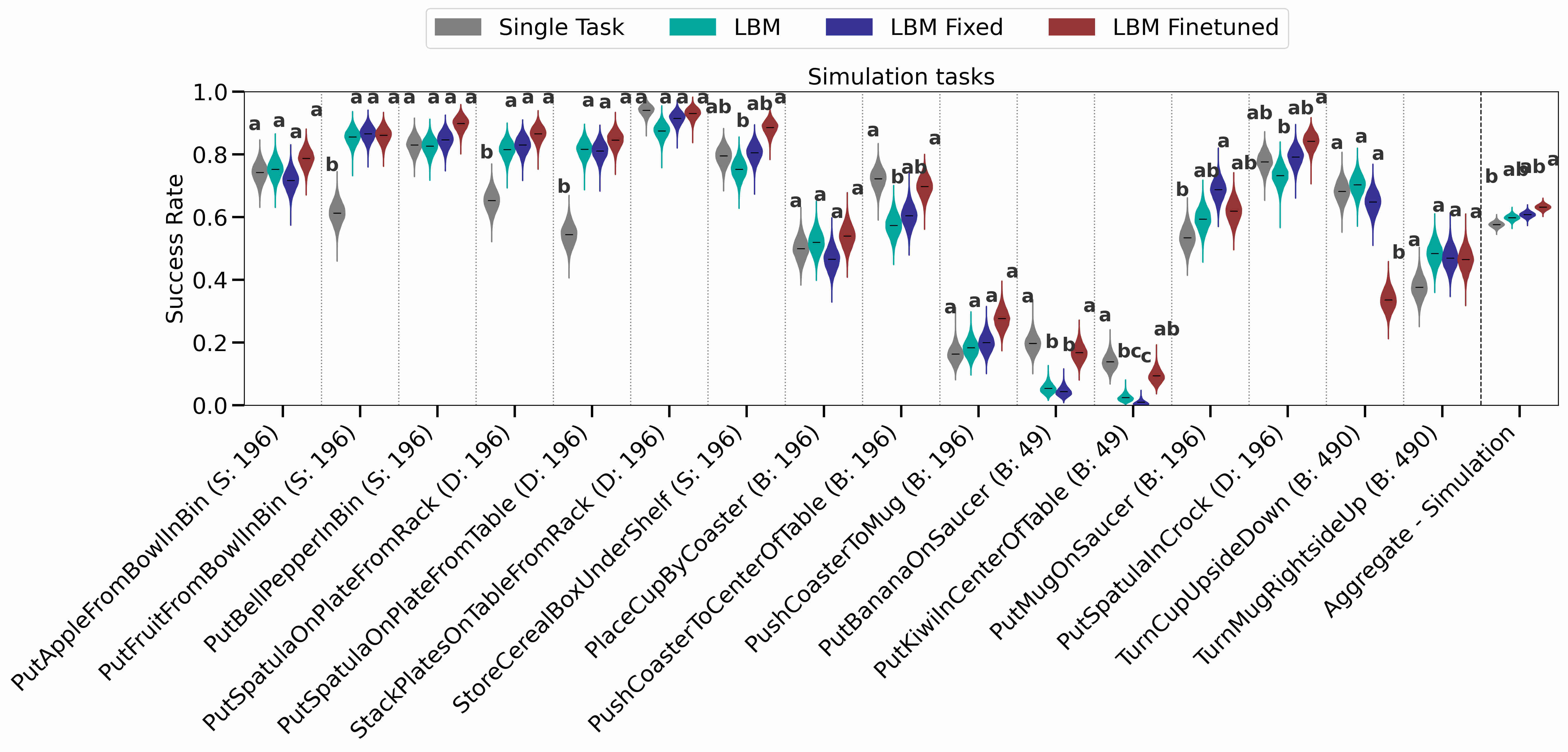
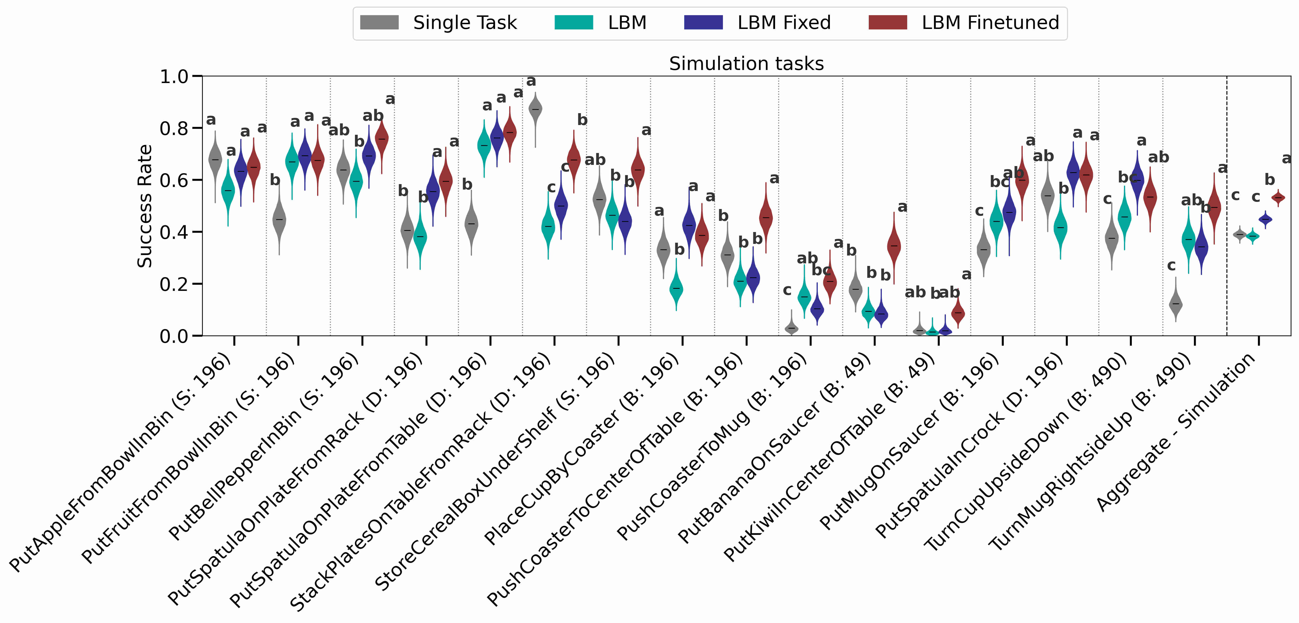
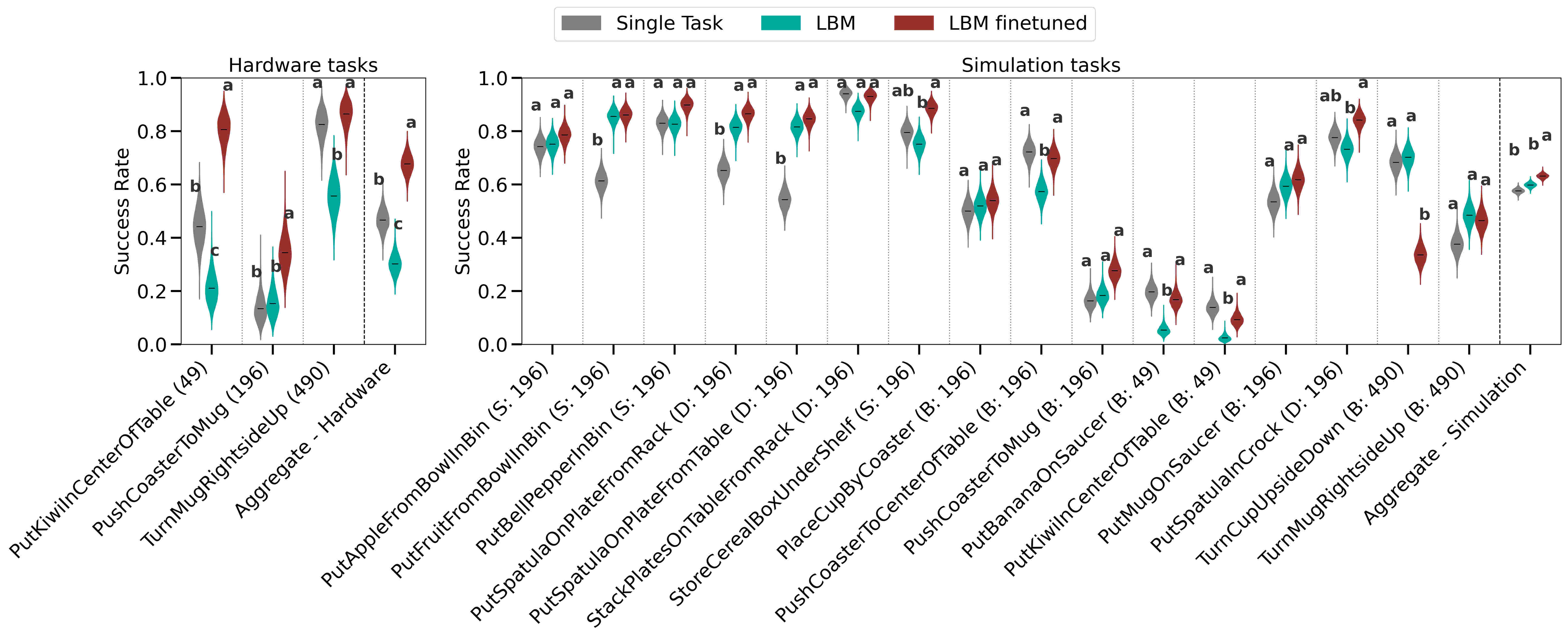
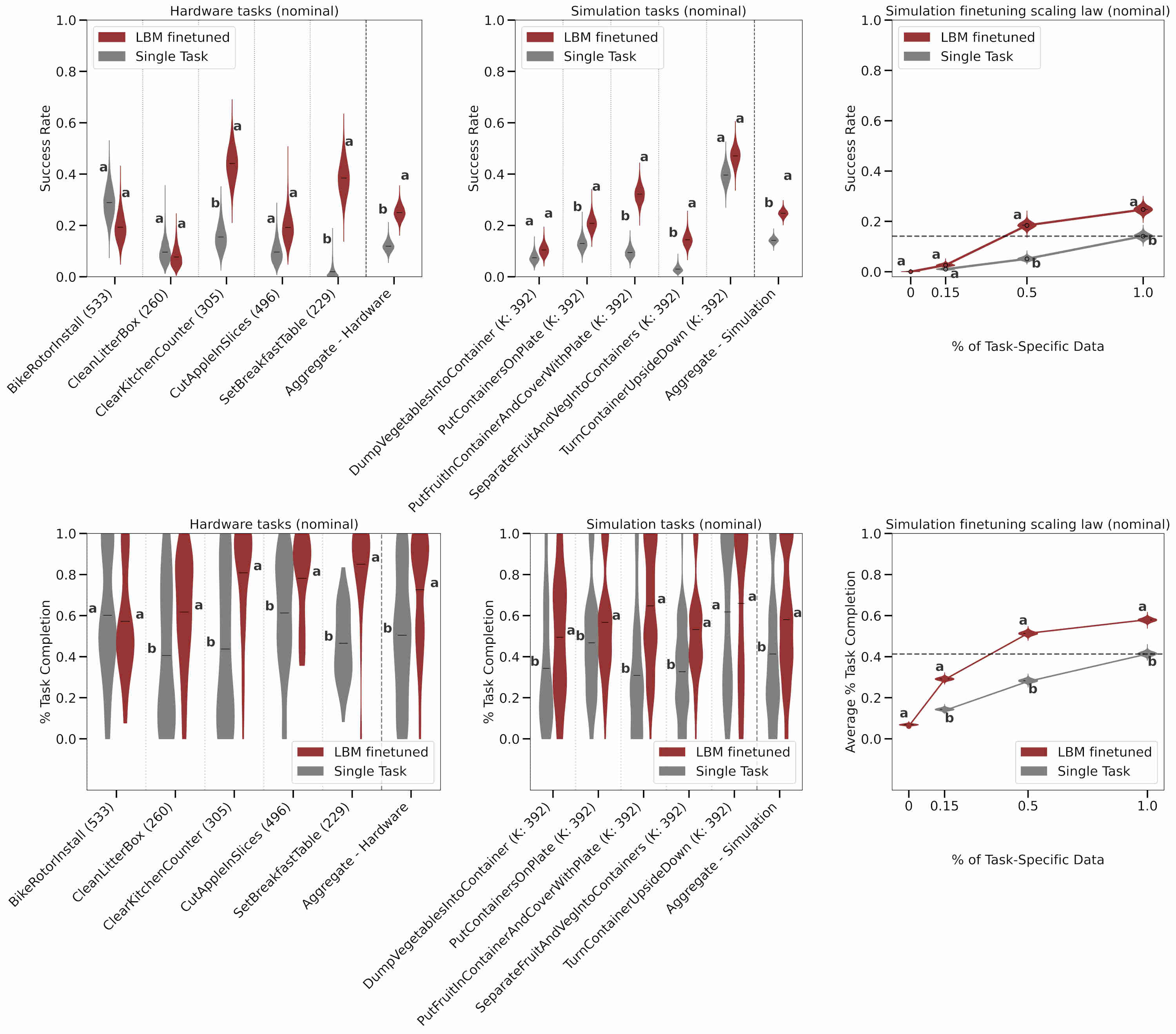
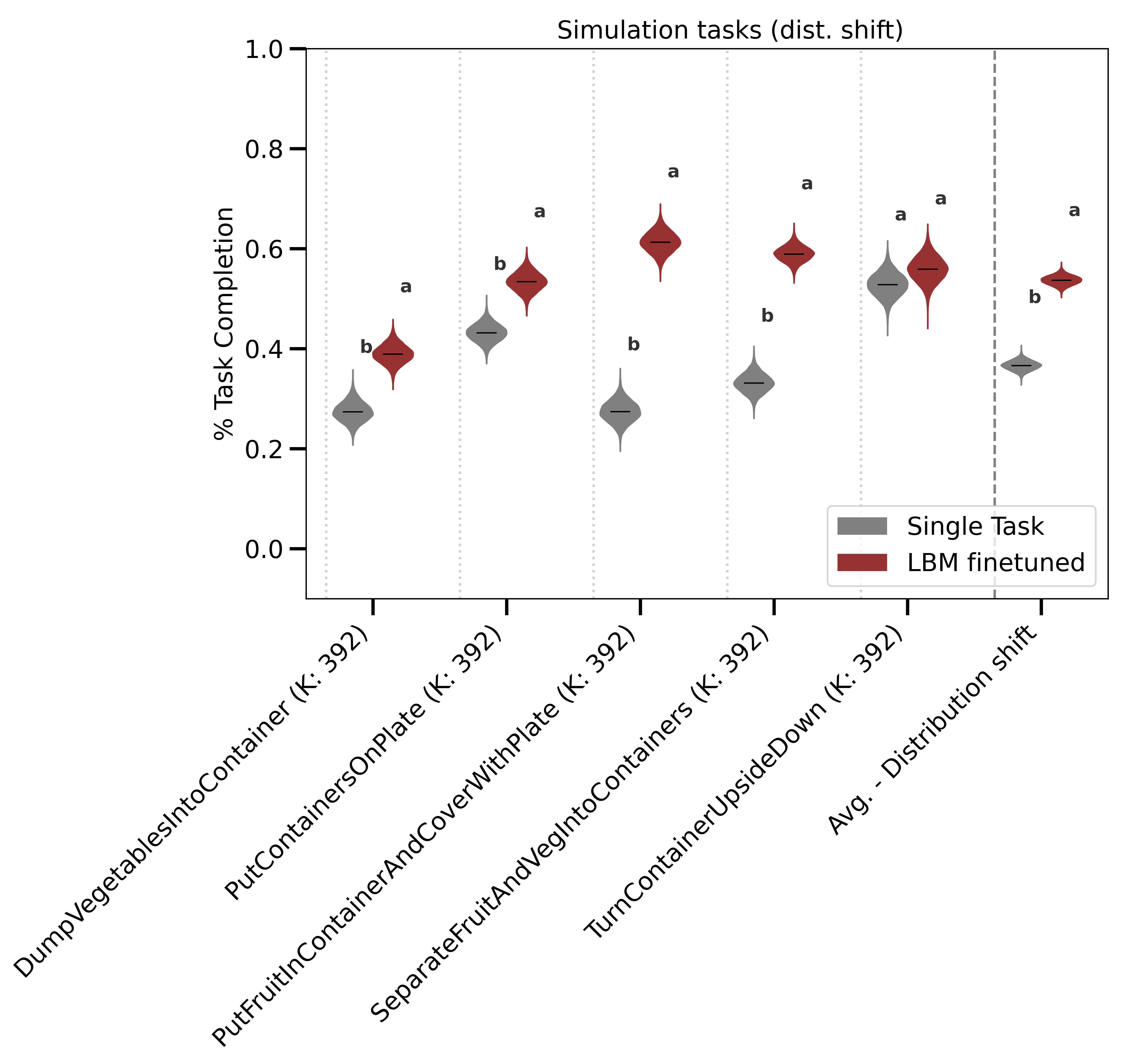
Success violins depict uncertainty in a probability, while individual-task completion violins depict the distribution of rollout scores. Aggregated completion plots instead show posterior uncertainty in the mean. All uncertainty is conditional on the selected policy checkpoints and excludes variation from retraining. Shared significance letters mean a difference was not established, not that policies are equivalent.
3.1 LBM performance on “seen” tasks
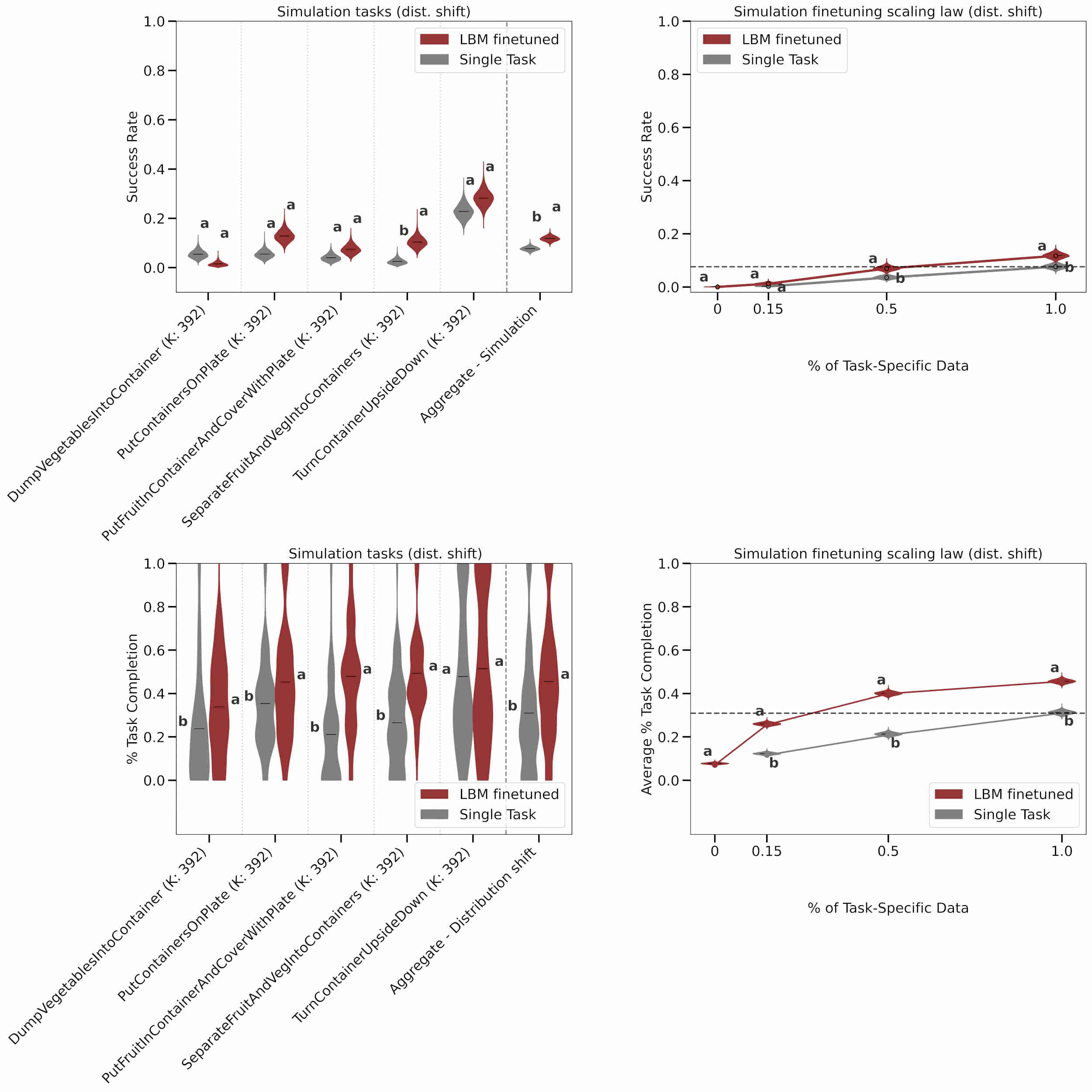
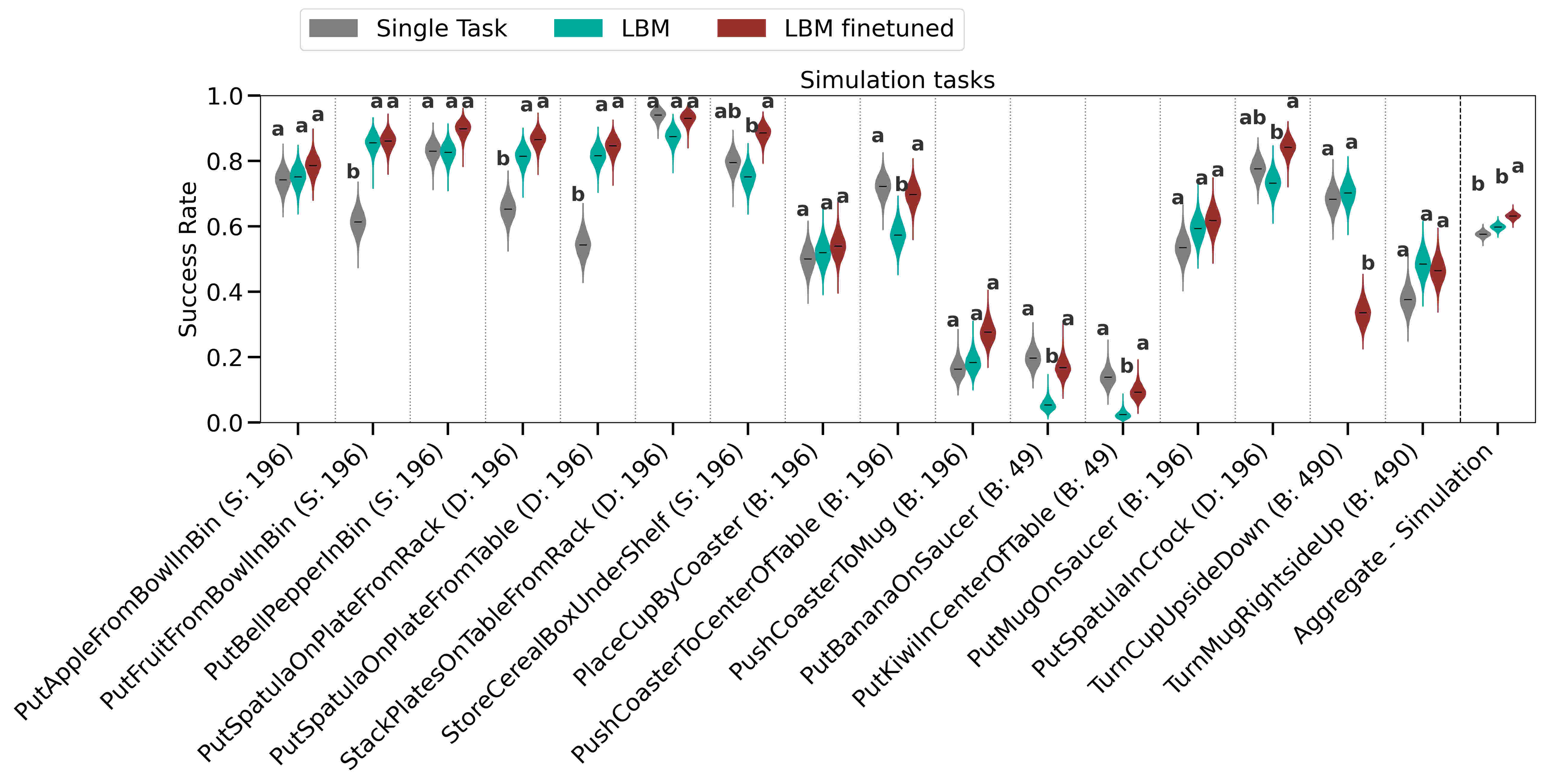
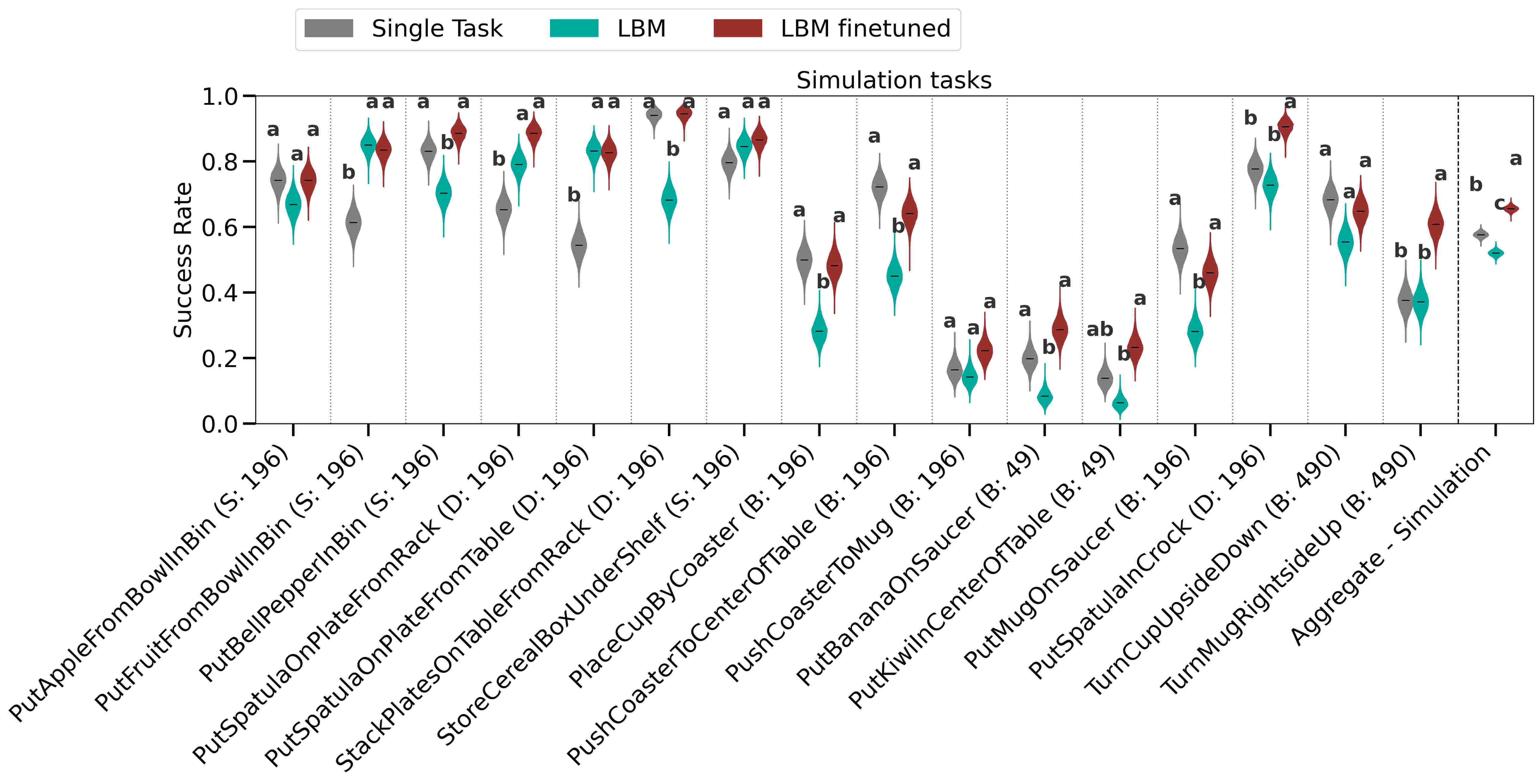
On seen tasks, fine-tuning improves aggregate success over the single-task baseline in simulation and hardware, including tested shifts. In simulation, significantly better performance expands from three of 16 nominal tasks to ten of 16 shifted tasks. Unadapted multitask models are mixed: they sometimes match or exceed single-task training, but do not consistently improve hardware performance.
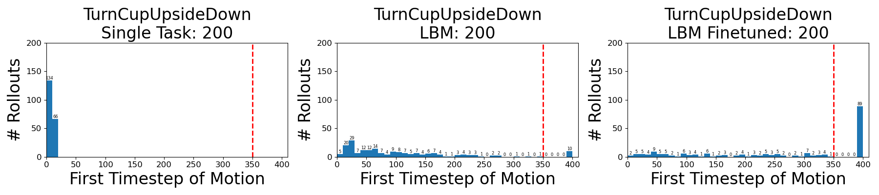
There are negative-transfer exceptions. The nominal TurnCupUpsideDown specialist succeeds in 33.5% of trials and fails to initiate motion in 89 of 200; a different plate-stacking task underperforms under shift. Sparse demonstrations, language confusion, and timeouts explain some other failures. The reported hardware shift comparisons combine task–condition instances rather than five distinct seen tasks. Simulation and physical shift procedures differ and should not be treated as identical tests.
3.2 LBM performance on “unseen” tasks
Held-out evaluation comprises three short simulation tasks, five complex simulation tasks, and five complex hardware tasks. Fine-tuned models improve aggregate success and milestone completion; on the complex hardware tasks they separate from the baseline on two of five success metrics and four of five completion metrics. Long-horizon success remains low despite better partial progress.
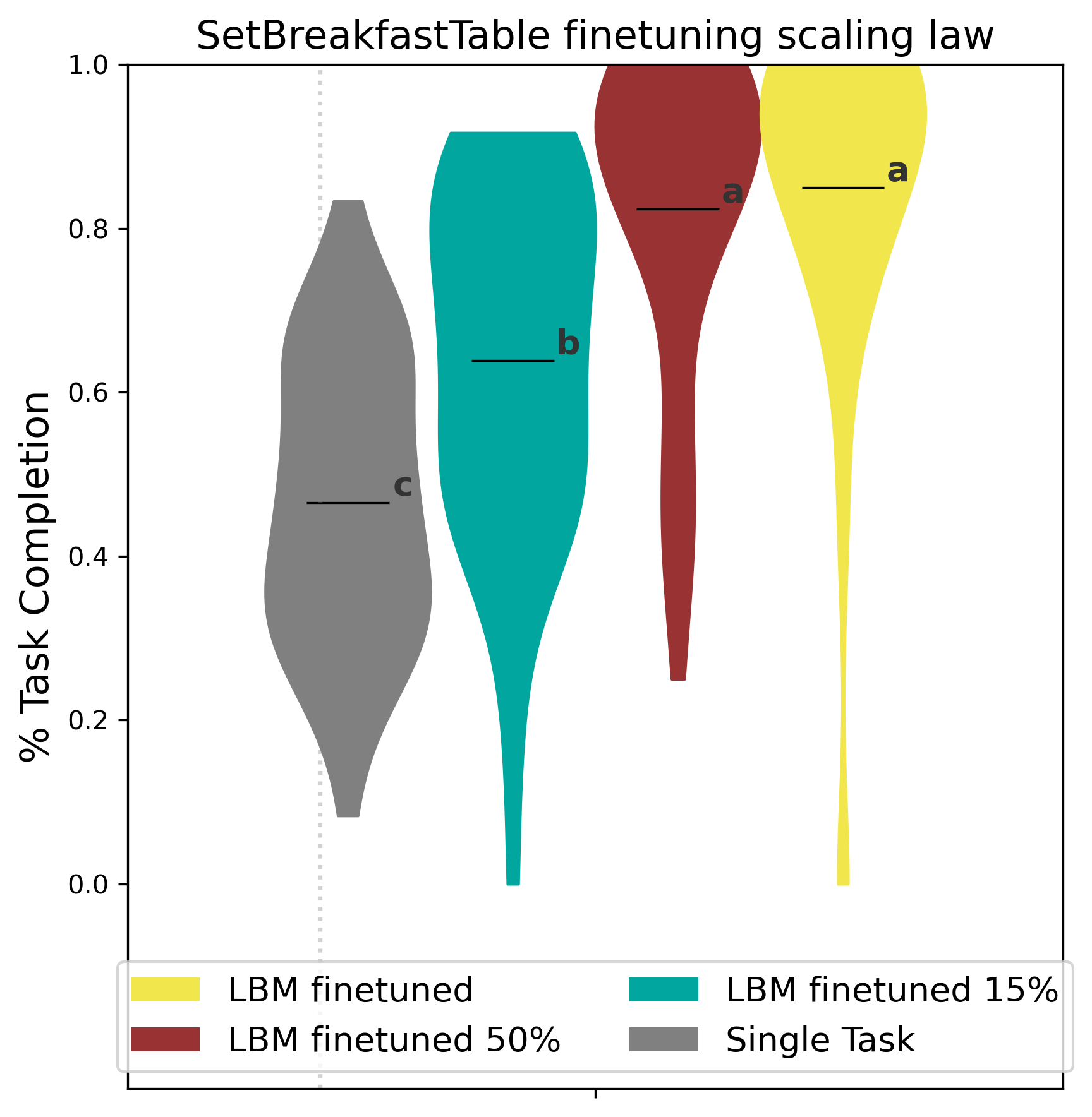
Interpolated simulation curves suggest comparable performance with under 30% of the baseline’s task-specific data. On the single physical breakfast-setting task, fine-tuning with 15% of the demonstrations exceeds the full-data baseline in task completion. This is task-dependent data efficiency, not a universal multiplier. The breakfast baseline has zero observed successes even though a posterior visualization can place probability mass above zero.
3.3 Pretraining scaling laws
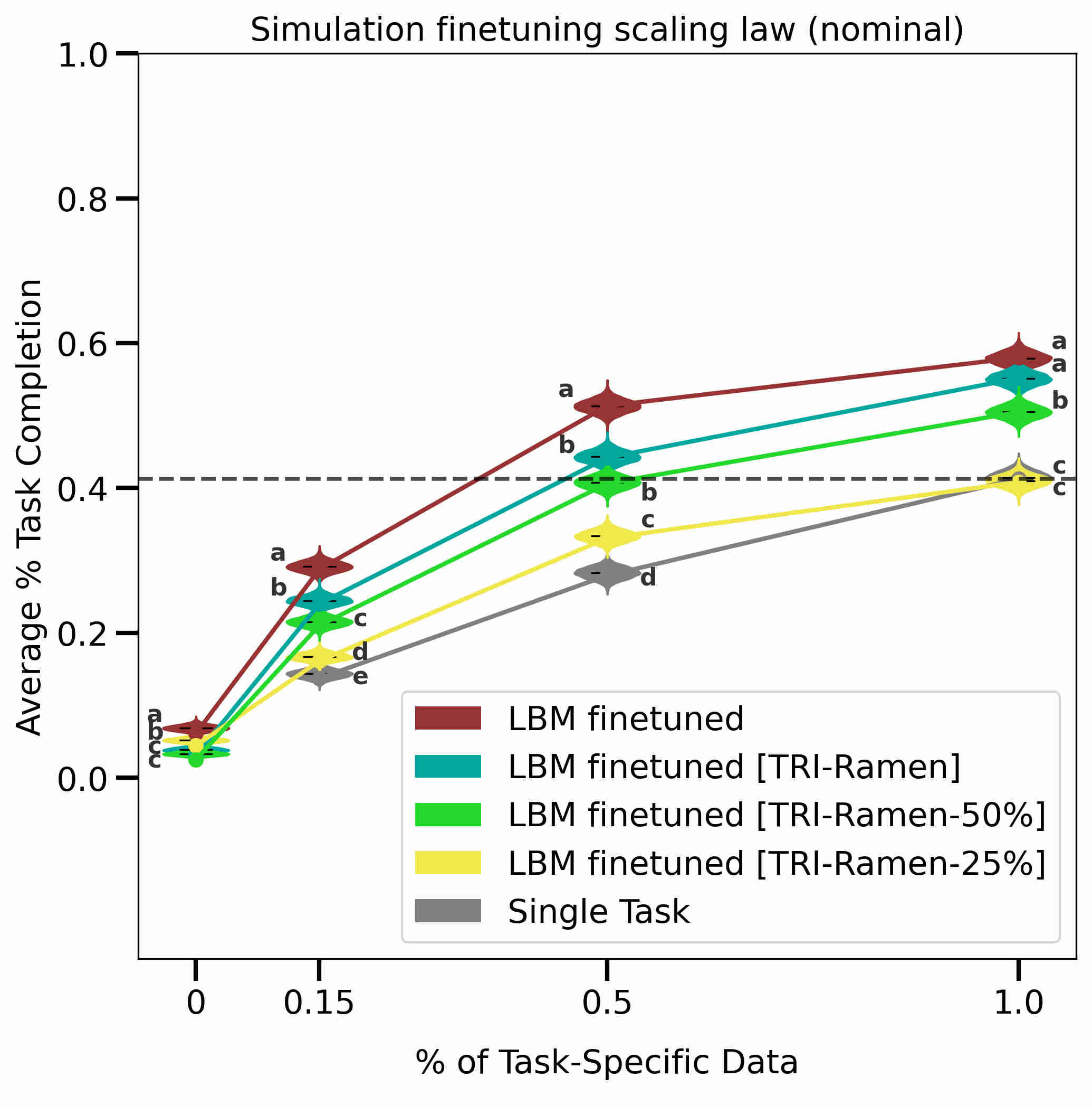
The simulation ablation varies robot pretraining: all internal plus public data, all internal data, and subsets containing 50% or 25% of internal tasks. All models share an architecture and are evaluated after several amounts of task-specific fine-tuning. More extensive pretraining generally improves mean completion, with especially clear separation when target-task data is scarce.
These experiments change task diversity and data volume together; they do not isolate those effects or fit a universal power law. Greater task-specific coverage narrows some pretraining gaps. The source occasionally calls the x-axis fraction “pretraining data,” but the plot varies fine-tuning data along that axis.
4 Materials and Methods
The methods specify how policies are compared, how diffusion-based models are trained, how data is standardized, and which tasks and shifts define the benchmark.
4.1 Evaluation Protocol and Analysis
The evaluation protocol aims to make policy differences interpretable through matched initial states, blinded randomized ordering, milestone scoring, independent scoring checks, and statistical comparison. It reduces experimental noise without eliminating it.
4.1.1 Policy comparison protocol
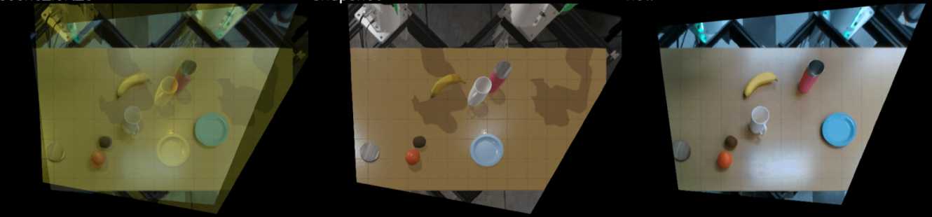
Simulation policies share evaluation seeds drawn separately from training initial states. Hardware trials run in bundles: each policy receives the same target scene, execution order is randomized, and operators do not know policy identity. Image overlays guide scene resets; a new scene is sampled only after the bundle finishes. This controls local conditions within human reset accuracy.
4.1.2 Rubrics and predicates
Human-scored yes/no milestones and failure questions describe hardware rollouts. Completion is the fraction of required milestones achieved. Simulation logs Boolean predicates over state, allowing both final success and partial progress to be computed. The chosen predicates and rubrics encode a task designer’s notion of progress, rather than an exhaustive measure of manipulation quality.
4.1.3 Rubric QA
A separate group rechecked about 27% of nearly 2,700 hardware rollouts, including earlier iterations beyond the 1,800 main-result trials. Success labels disagreed in 2.31% of cases and individual rubric answers in 6.25%. Five rollouts were corrected before analysis. These checks estimate labeling consistency; they do not eliminate setup errors or all scoring ambiguity.
4.1.4 Statistical Analysis: Performance Characterization of Individual Policies
Uncertainty visualizations characterize repeated evaluation of each fixed trained checkpoint. They should be distinguished from uncertainty over training runs or population-level generalization.
Binary Success/Failure Criteria
Binary success is modeled as a Bernoulli outcome with a uniform Beta prior, yielding a posterior violin after observing trials. Matched random seeds and randomized hardware bundles support controlled comparisons. Pooling a fixed number of trials from each task departs from strict independent identical sampling; the authors treat this as a practical approximation. Overlapping marginal intervals do not rule out a significant paired difference.
Task Completion Criteria
Milestone completion can be multimodal, so individual-task violins show actual rollout-score distributions. For mean completion in fractional-data or aggregate analyses, a uniform Dirichlet prior supplies posterior uncertainty. A high average can still conceal many incomplete rollouts, which is why raw distributions and binary success are both useful.
4.1.5 Statistical Analysis: Performance Comparison of Multiple Policies
Pairwise policy tests receive a Bonferroni correction within each comparison group, with compact-letter displays summarizing separation. Binary outcomes use a sequential paired test; completion means use Welch’s t-test as a large-sample approximation for discrete scores.
The correction is not extended across every task in a figure, so the many task-level conclusions do not have a single global 5% error guarantee. The completion test and pooled-task assumptions are also approximate. These qualifications limit how broadly one should read individual significance letters.
Related source: sequential policy comparison.
4.2 Large Behavior Models
The policy is a conditional diffusion model with fixed transformer capacity. Comparisons change the amount and source of robot training rather than network architecture.
4.2.1 Diffusion for Visuomotor Control
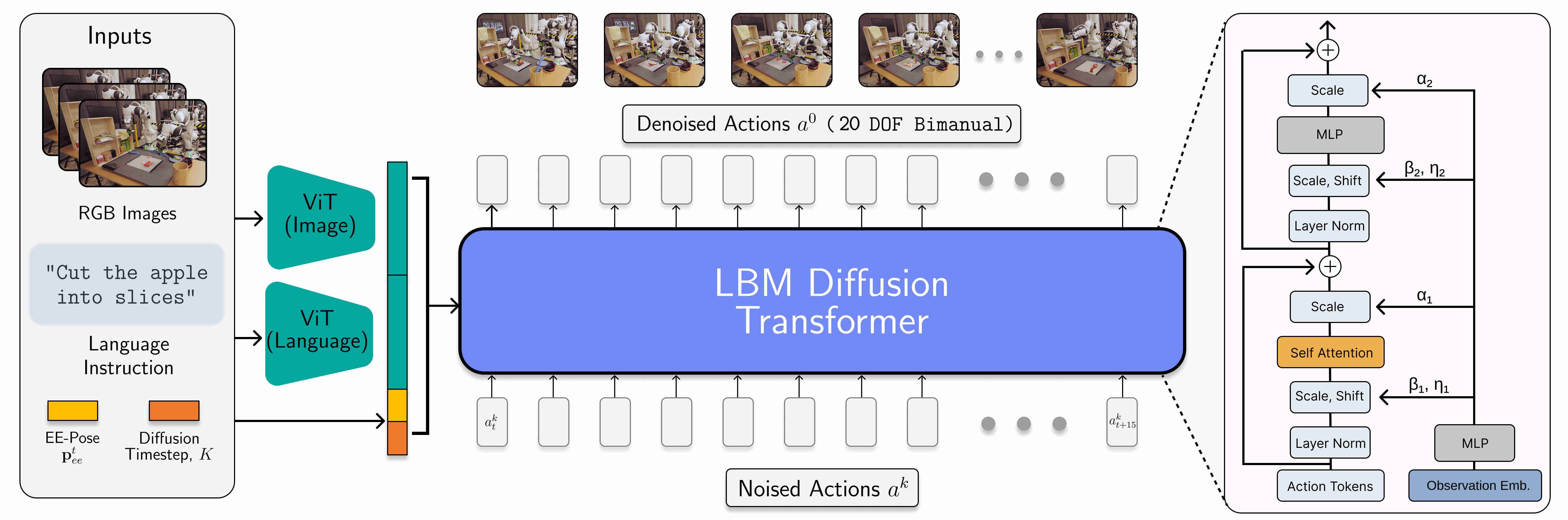
A denoising network transforms sampled Gaussian action noise into a continuous action sequence conditioned on images, proprioception, and language. Training predicts the injected noise; deployment uses iterative DDIM denoising. This extends the action-diffusion approach to a heterogeneous multitask corpus.
Related source: Diffusion Policy.
Equations 1–2
| (1) |
| (2) |
4.2.2 Policy Architecture
A shared CLIP vision encoder supplies image features, a frozen CLIP text encoder supplies language features through a trained projection, and proprioception and diffusion-step embeddings condition eight transformer blocks of width 768 through adaptive normalization. Two observation times condition a prediction of 16 action steps, each with 20 bimanual action dimensions.
The visual encoder is fine-tuned, while the language encoder stays frozen. Single-task baselines use the same architecture and feature setup; “from scratch” refers to lacking multitask robot pretraining, not necessarily lacking all pretrained visual-language knowledge.
Related source: Diffusion Transformers.
4.2.3 Training and Deployment
Pretraining uses 48,000 steps, batch 2,560, and learning rate 3×10⁻⁴, with a tenfold smaller rate for the vision encoder. Fine-tuning uses batch 320 and 2×10⁻⁵ for 30,000 hardware or 10,000 simulation steps. Table 1 gives longer single-task runs: 100,000 and 25,000 steps, respectively, so this is not a matched-compute comparison.
Training resizes images to 256×342, randomly crops to 224×224, and applies color jitter; deployment uses a center crop. The system predicts 16 steps and executes eight before replanning, with the reported control rate of 10 Hz. All augmentation and architecture settings remain in the original tables.
| Hyperparameters | Pretraining | Finetuning (Real) | Finetuning (Sim) | Single-Task (Real) | Single-Task (Sim) |
|---|---|---|---|---|---|
| Learning Rate | 3e-4 | 2e-5 | 2e-5 | 2e-5 | 2e-5 |
| Global Batch Size | 2560 | 320 | 320 | 320 | 320 |
| Steps | 48000 | 30000 | 10000 | 100000 | 25000 |
| LR Schedule | Constant | Constant | Constant | Constant | Constant |
| Hyperparameters | Values |
|---|---|
| Image Augmentation | |
| Resize (HxW) | 256x342 |
| Random Crop (HxW) | 224x224 |
| Brightness Range | [0.8, 1.2] |
| Contrast Range | [0.6, 1.4] |
| Saturation Range | [0.8, 1.2] |
| Hue Range | [-0.05, 0.05] |
| Model Architecture | |
| DiT Layers | 8 |
| DiT Embedding Dimension | 768 |
| CLIP Image Encoder | ViT-B/16 |
4.3 Experimental Details
The experiments use a bimanual tabletop robot fleet and a corresponding Drake-based simulation benchmark, with different levels of scene matching and control.
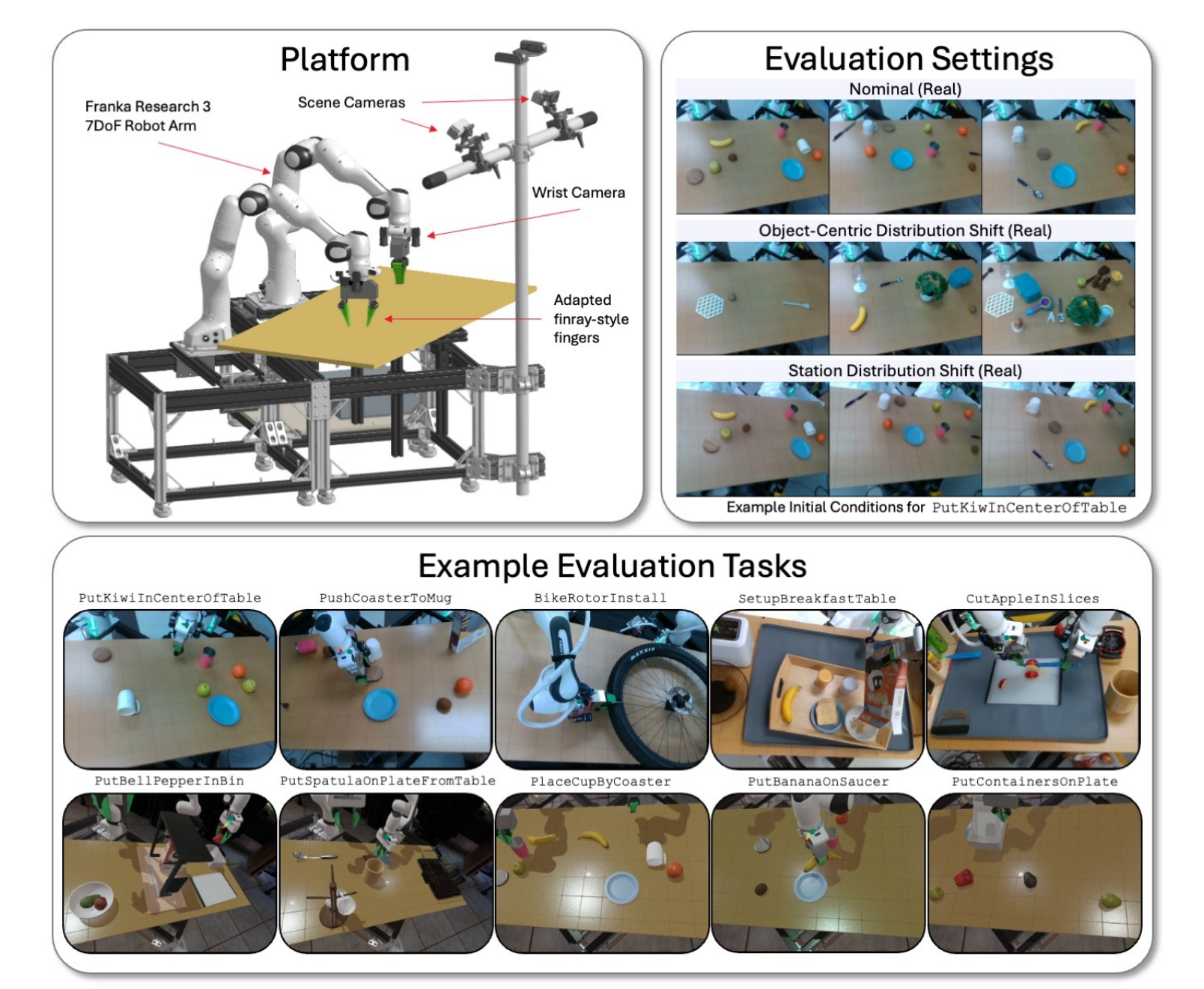
4.3.1 Platform
Two Franka FR3 arms, compliant fingers, parallel grippers, scene cameras, and wrist cameras form each station. Differential inverse kinematics converts relative end-effector commands to a joint-impedance controller and handles collision avoidance. Demonstrations span nine hardware stations and two hardware generations; reported physical evaluations use the newer grippers and four wrist cameras.
4.3.2 Simulation
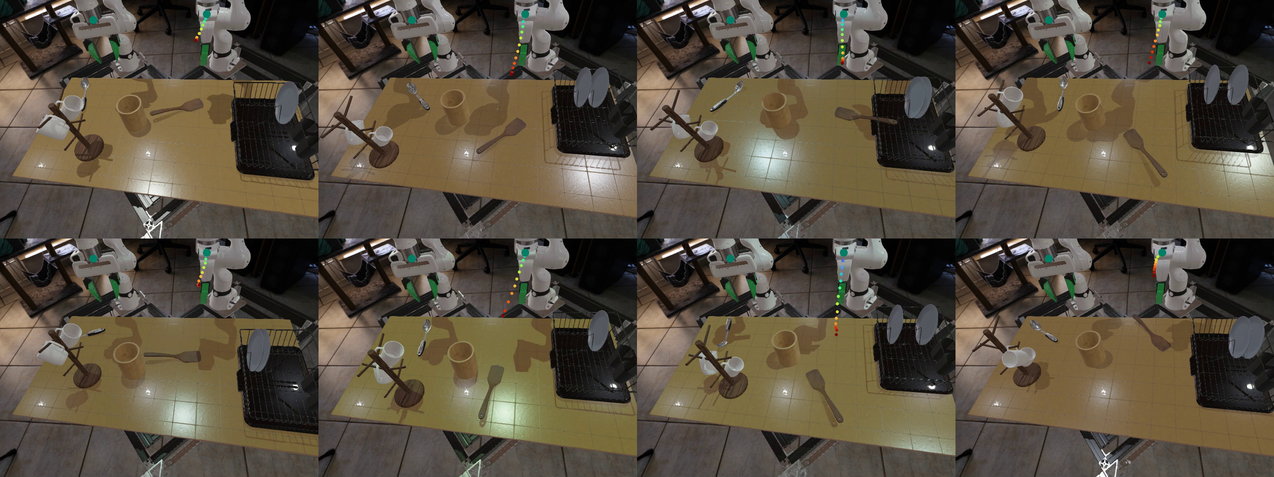
The lbm_eval simulator contains DryingRack, Shelf, Breakfast, and Kitchen scenarios. They differ in objects, clutter, and task complexity; Kitchen supplies held-out long-horizon tasks. A simple box-moving debug scenario contributes pretraining data but is not evaluated. Seeds make simulated scenes repeatable, though GPU policy inference is not guaranteed deterministic. The simulator is behaviorally matched to hardware, not an exact physical replica.
4.4 Pretraining data
The Ramen mixture totals about 1,695 demonstration hours: 545 internal and 1,150 curated public hours. Internal data comprises 468 hardware hours across 362 tasks, 45 simulation hours across 41 tasks, and 32 handheld-interface hours across 129 tasks, totaling 64,262 demonstrations. Thus the internal total includes simulation despite one sentence calling it all real data.
The held-out Kitchen tasks and one task each from the other three scenarios are excluded from robot pretraining. Public datasets are chosen heuristically, mapped into common camera/action formats, and balanced by explicit batch weights. Dataset hours therefore do not equal sampling probability during training.
Related source: the Universal Manipulation Interface.
4.4.1 Observation and Action spaces
Observations combine two times of end-effector poses, relative arm geometry, gripper widths, up to six RGB images, and a language instruction. Actions describe relative end-effector trajectories and gripper widths using a continuous six-dimensional rotation representation. Missing cameras or arms are zero-padded; unimanual episodes randomly swap arm side.
Internal instructions include a human description and five language-model paraphrases; missing public instructions receive a generic prompt. The observation subsection states a horizon of 15 while the architecture and training describe 16 predicted timesteps; the source does not explicitly explain that indexing convention.
4.4.2 Data Normalization
Per-feature, per-time normalization maps the second and 98th percentiles to −1 and 1, clipping at ±1.5 while leaving rotation features unchanged. Separate source normalizers account for different action scales; future relative actions receive their own statistics.
A pretraining bug applied some samples’ normalizers from the wrong dataset. The full hardware study was not repeated. A smaller corrected-model simulation experiment finds little nominal difference but stronger shifted-condition performance. Consequently the main reported models include this known data-processing error; the follow-up does not revalidate every fine-tuned or physical result.
Equation
4.4.3 Dataset filtering
Initial idle frames are removed until movement exceeds 5 cm or 15 degrees. This helps simulation policies initiate motion, but filtering pretraining also makes unadapted models more likely to execute the wrong task. Main pretraining therefore uses unfiltered data, while simulation fine-tuning and single-task training use filtered data. Hardware task-specific data remains unfiltered. These asymmetric data choices are part of the experimental recipe.
4.5 Evaluation Tasks
Simulation evaluates 16 seen tasks and eight held-out tasks; hardware evaluates three seen and five held-out tasks. Tables specify demonstration counts and which physical shifts are actually tested. The target trial count is 200 per simulation cell and 50 per hardware cell, subject to recorded missing simulation runs.
4.5.1 Simulation
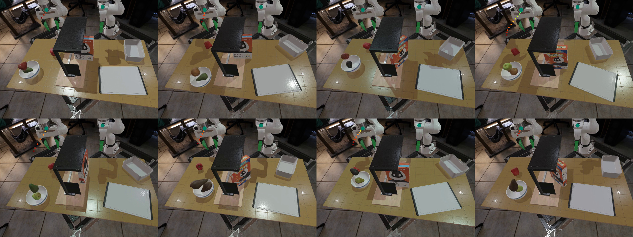
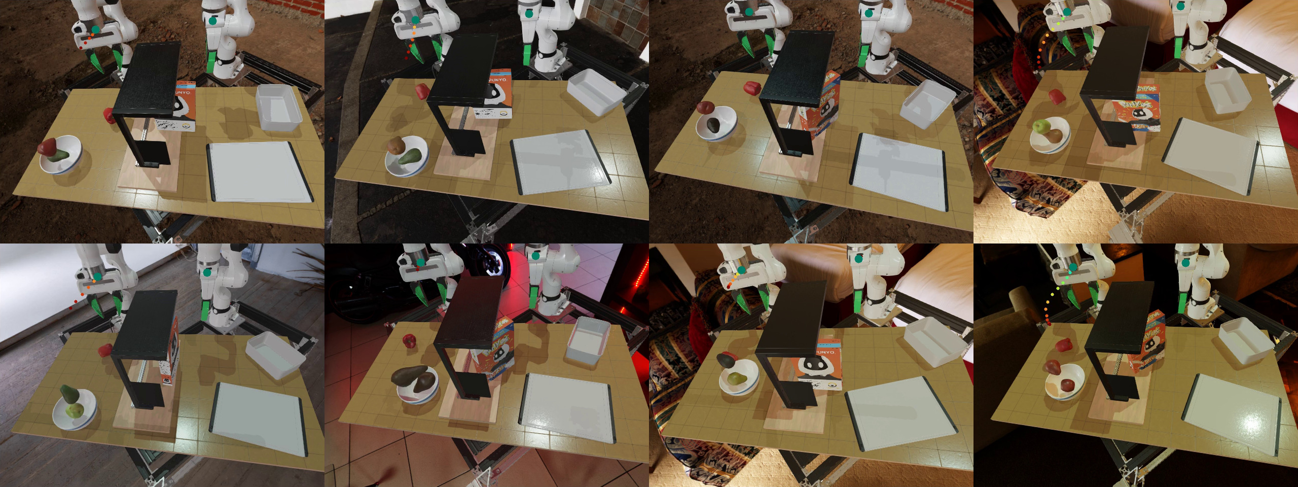
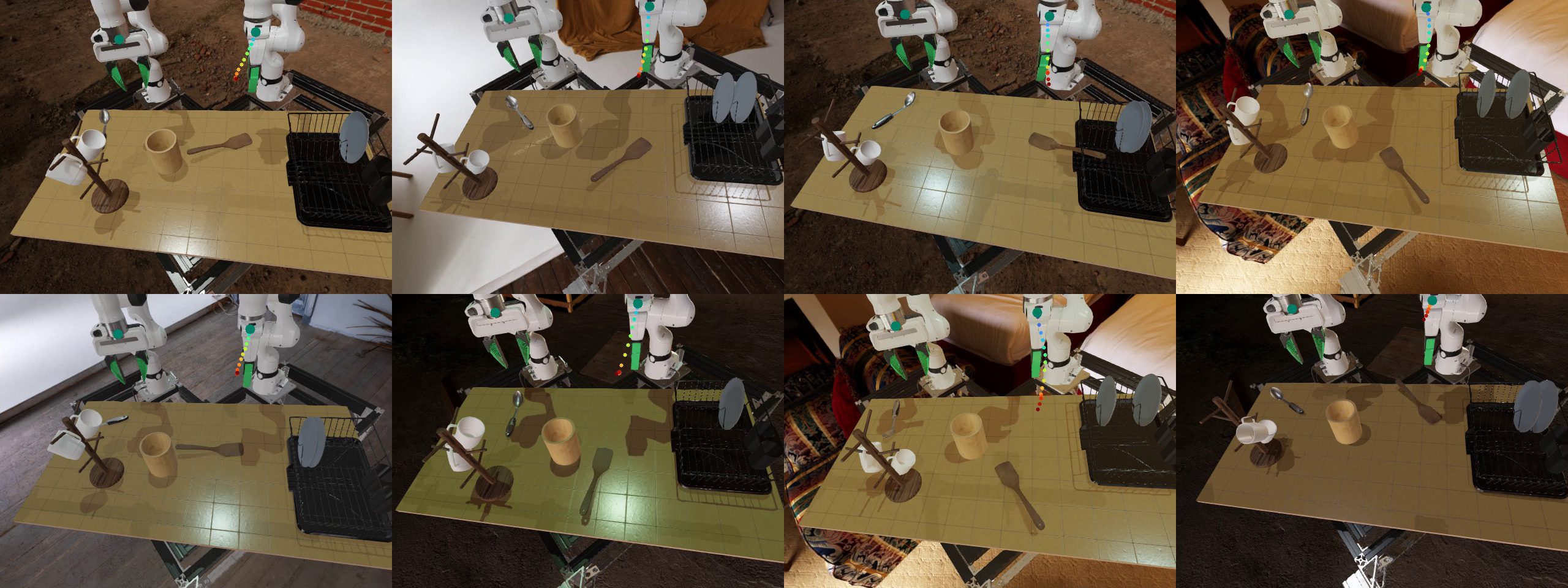
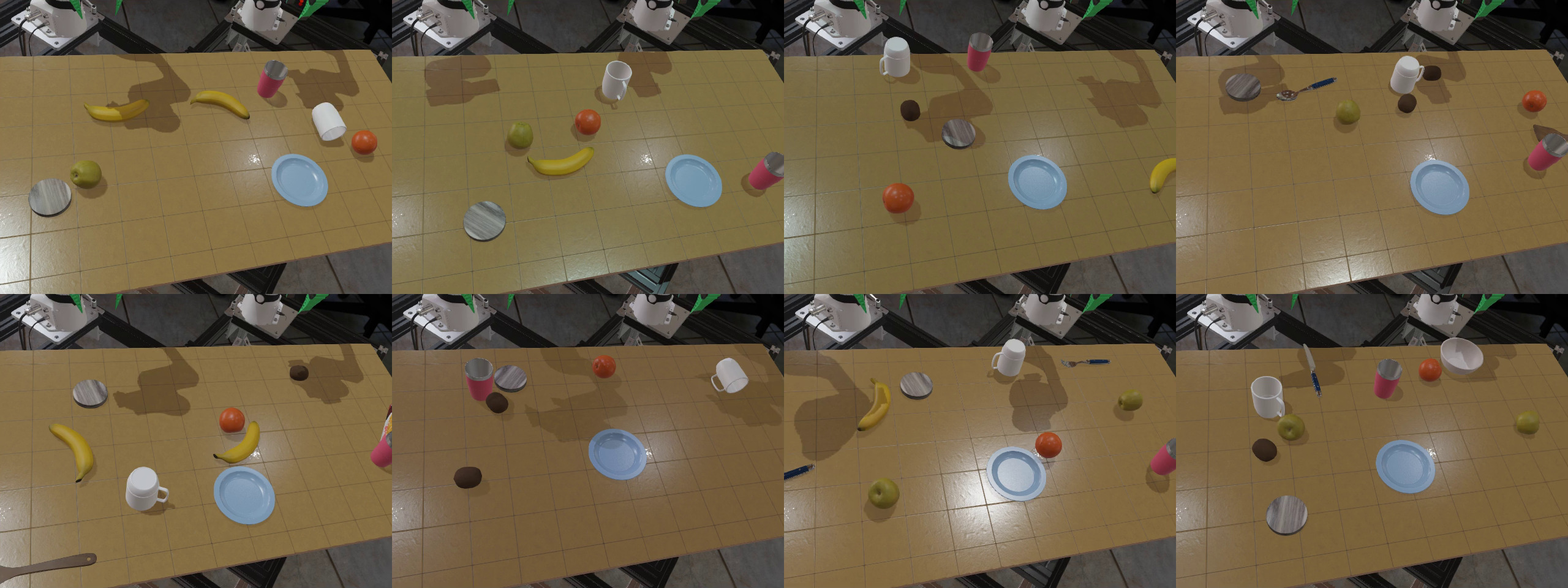
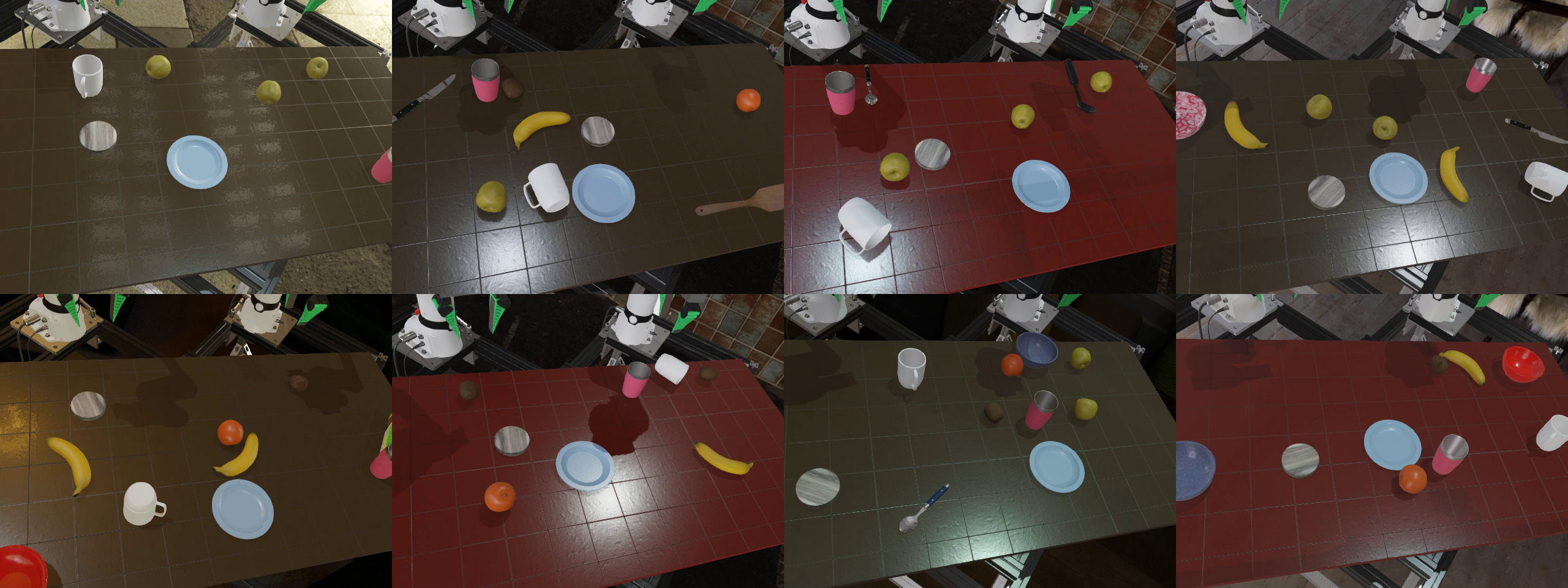
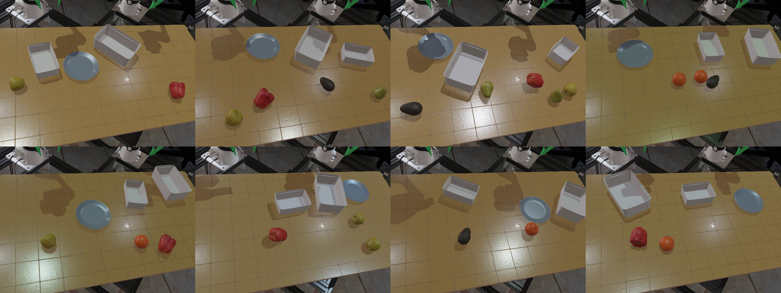
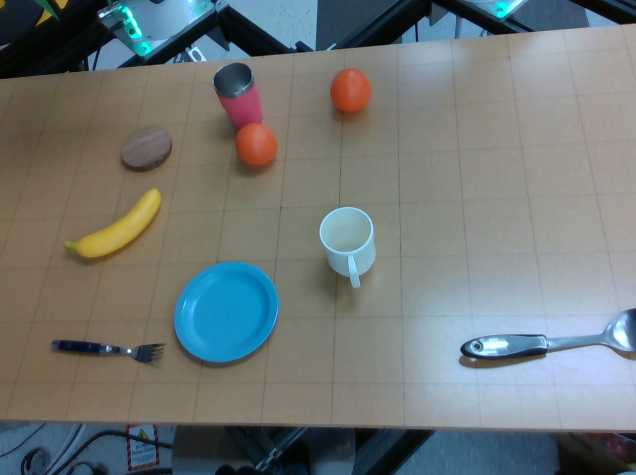
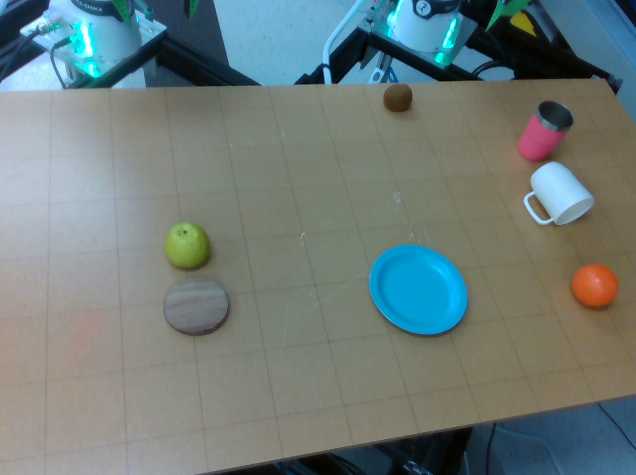
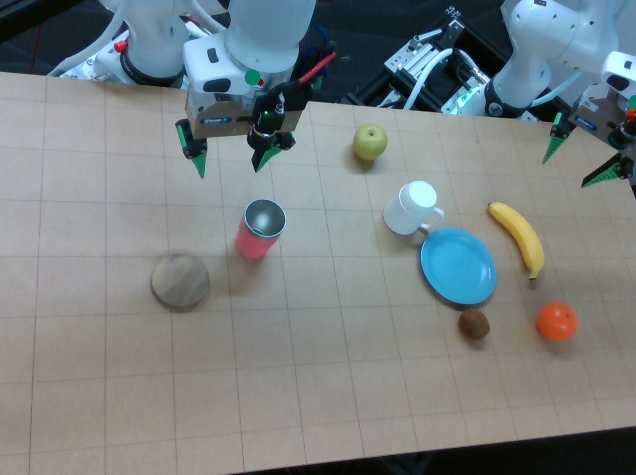
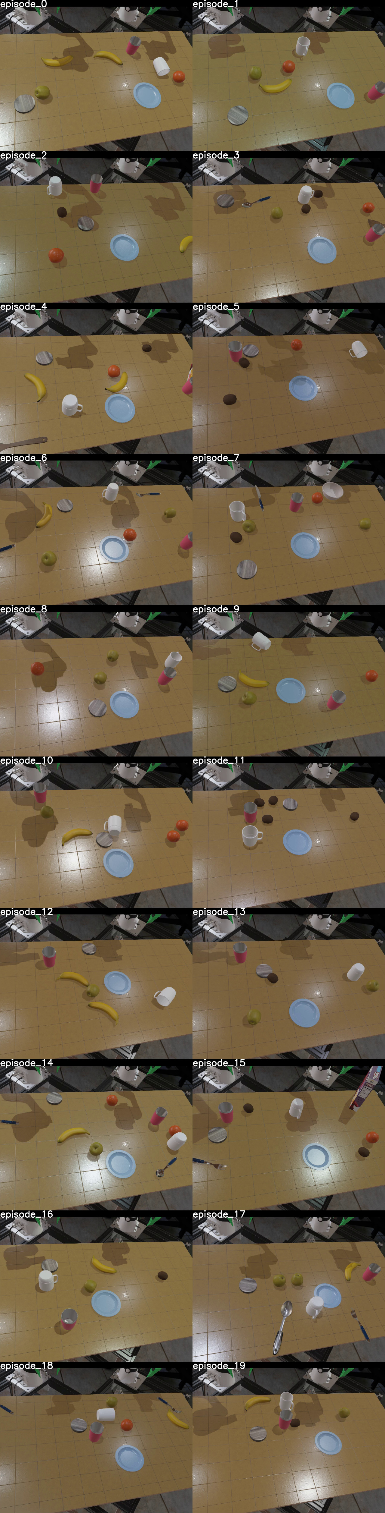
Nominal simulation randomizes poses, object quantities, and lighting within training distributions. Shifted trials change environment maps, an additional light source, camera parameters, textures, colors, and in Breakfast some distractors. Visually ambiguous initial scenes force policies to use language. The shifts are scenario-specific and mostly concern appearance rather than a general test of all dynamics changes.
4.5.2 Real
Hardware tests include familiar scenes, transfer to a station without that task’s fine-tuning demonstrations, and novel object/distractor instances. A new station need not be globally absent from pretraining. Selected shifts are practical to stage and were chosen to avoid near-universal failure, limiting their coverage of difficult deployment conditions.
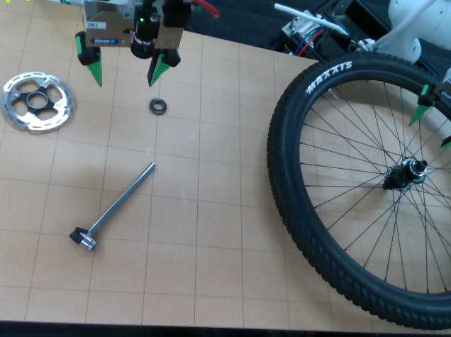
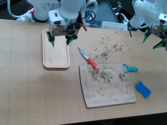
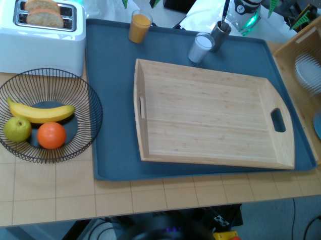
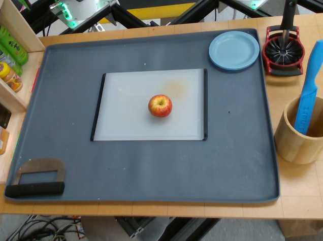
Complex tasks include precise rotor installation, breakfast preparation, and a long apple-coring/cutting/cleanup sequence. Novel-object status is based on the authors’ best knowledge of the large pretraining mixture, not a formal guarantee of no prior exposure.
5 Discussion and Conclusion
The main evidence supports broad robot pretraining followed by task-specific adaptation: better aggregate outcomes and often several-fold lower target-demonstration requirements. Unadapted multitask models remain inconsistent, partly through poor language steering and idle behavior. Data-scale curves improve smoothly over the tested range without a demonstrated sharp transition.
The study also shows why careful evaluation and data processing matter: small effects can be hidden by experimental noise, and normalization or filtering can materially change results. These conclusions concern the tested fixed architecture and datasets rather than all large robot models.
5.1 Limitations
The statistical analysis conditions on selected trained weights and omits variation between training seeds. More rollouts narrow evaluation uncertainty without resolving that missing source of variation. Hardware reset and scoring errors remain despite overlays and quality checks, and the protocol trades throughput for control. The modest frozen CLIP language encoder also limits extrapolation to models with much larger language backbones.
Equation
Supplementary Materials for A Careful Examination of Large Behavior Models for Multitask Dexterous Manipulation
The supplement accompanies the same TRI LBM Team study and provides the operational details and additional analyses summarized below.
6 Authors and contributions
The team credits 23 primary contributors for policy architecture/training, evaluation, and simulation; a larger group contributes infrastructure, data collection, and review. Project leadership is credited to Rares Ambrus, Kerri Fetzer-Borelli, Ben Burchfiel, Hadas Kress-Gazit, Siyuan Feng, Stacie Ford, and Russ Tedrake. Most authors are affiliated with Toyota Research Institute, with Kress-Gazit at Cornell.
7 Platform Details
Table S1 records which hardware and simulated stations contribute demonstrations or evaluations, and distinguishes retired from current hardware.
7.1 Robot Hardware
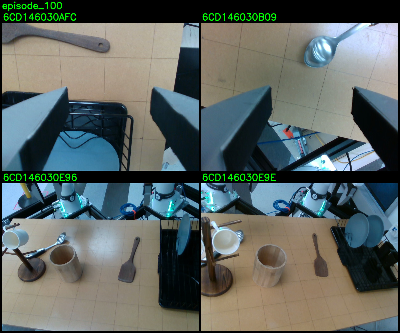
The upgrade replaces the Franka Hand with a Schunk gripper, replaces one wrist camera per arm with two, and shortens compliant fingers. Retired stations still contribute data but are not used in the reported physical evaluations. Weekly calibration reduces drift across camera and robot configurations, which remain meaningfully different between stations.
7.2 Simulated Robot
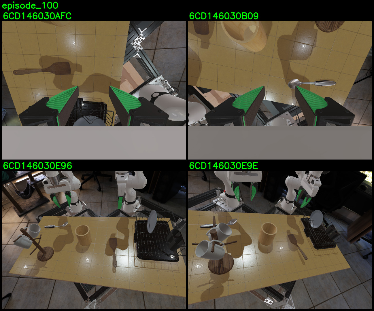
Simulation models the two hardware generations without exact visual or physical identity. Wide-angle views use rendered pinhole images followed by distortion; the older simulated station deliberately has wider fields of view for observability. These choices can alter task difficulty relative to hardware.
| Station Name | HW / Sim | Platform type | Data collection | Evaluation |
|---|---|---|---|---|
| cabot | sim | new | Yes | Yes |
| riverway (sim) | sim | old | Yes | Yes |
| wood_island | HW | new | Yes | Yes |
| hersey | HW | new | Yes | Yes |
| maverick | HW | new | Yes | Yes |
| ruggles | HW | new | Yes | Yes |
| salem | HW | new | Yes | Yes |
| davis | HW | new | Yes | Yes |
| milton | HW | new | Yes | Yes |
| wollaston | HW | old | Yes | No |
| riverway (HW) | HW | old | Yes | No |
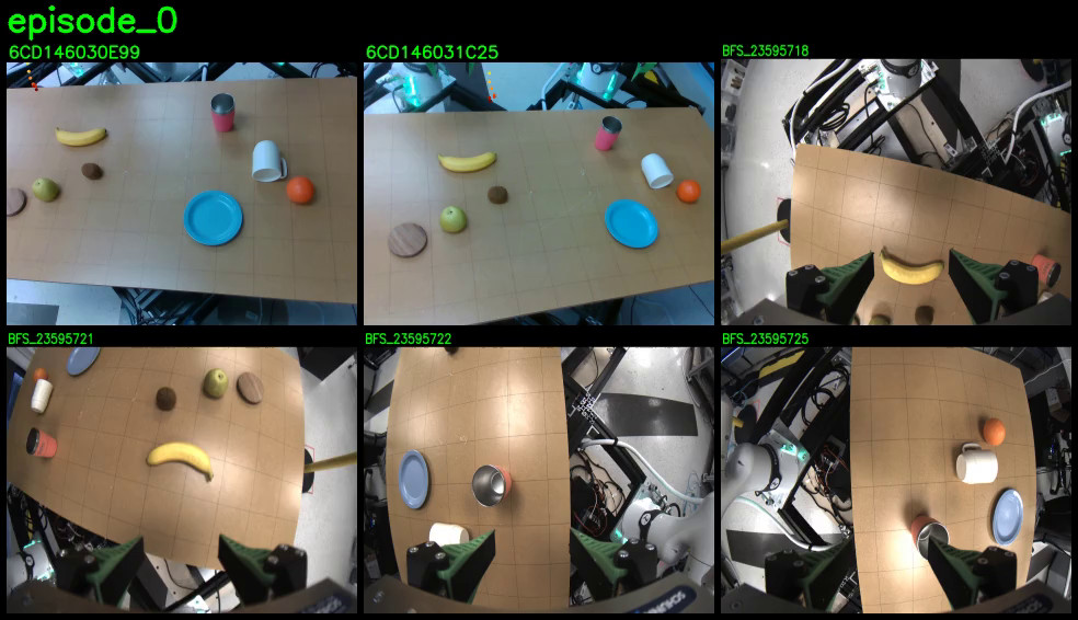
8 Simulation evaluation details
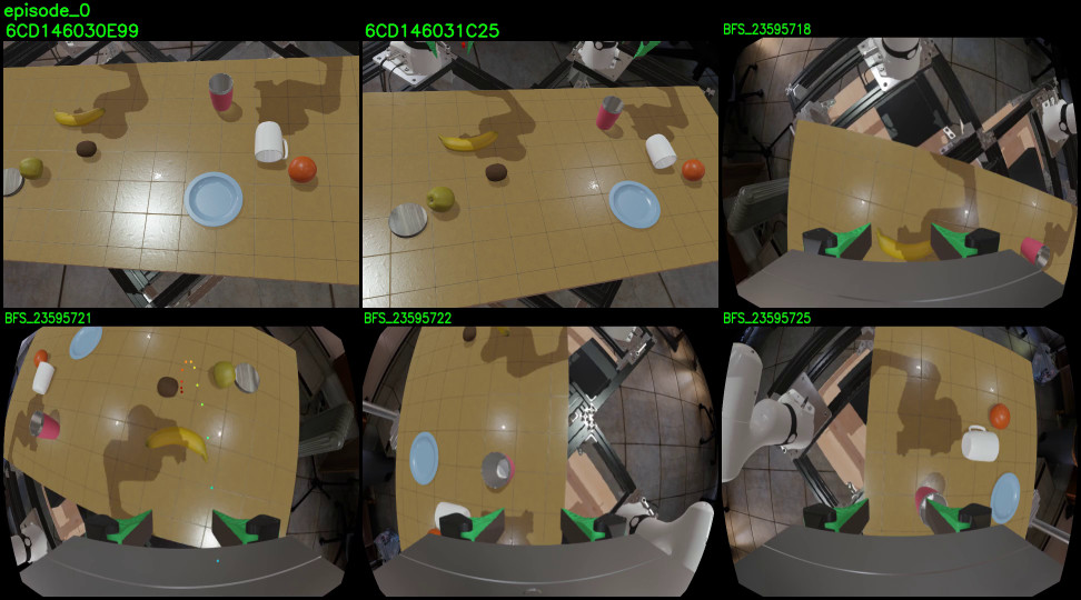
The supplementary simulation details connect each scenario to its station model and provide task counts, scene variation, predicates, and missing-run accounting.
8.1 Data used for training or finetuning during simulation evaluation
Table S2 provides task-specific demonstration counts, ranging from 49 for sparse seen tasks to 392 for each complex Kitchen task. The short appendix sentence mentions five unseen tasks, while the main results and table also include three shorter held-out tasks; the complete evaluation therefore has eight unseen tasks.
| Task name | Seen in pretraining | Scenario | riverway | cabot | Total |
|---|---|---|---|---|---|
| PutSpatulaOnPlateFromDryingRack | Seen | DryingRack (D) | 196 | 0 | 196 |
| PutSpatulaOnPlateFromTable | Seen | DryingRack (D) | 196 | 0 | 196 |
| StackPlatesOnTableFromDryingRack | Seen | DryingRack (D) | 196 | 0 | 196 |
| PutSpatulaInUtensilCrock | Seen | DryingRack (D) | 196 | 0 | 196 |
| PutSpatulaOnPlateFromUtensilCrock | Unseen | DryingRack (D) | 196 | 0 | 196 |
| PlaceAppleFromBowlIntoBin | Seen | Shelf (S) | 196 | 0 | 196 |
| PlaceFruitFromBowlIntoBin | Seen | Shelf (S) | 196 | 0 | 196 |
| PutBellPepperInBin | Seen | Shelf (S) | 196 | 0 | 196 |
| StoreCerealBoxUnderShelf | Seen | Shelf (S) | 196 | 0 | 196 |
| PlaceAvocadoFromBowlIntoBin | Unseen | Shelf (S) | 196 | 0 | 196 |
| PlaceCupByCoaster | Seen | Breakfast (B) | 0 | 196 | 196 |
| PushCoasterToCenterOfTable | Seen | Breakfast (B) | 0 | 196 | 196 |
| PutBananaOnSaucer | Seen | Breakfast (B) | 0 | 49 | 49 |
| PutMugOnSaucer | Seen | Breakfast (B) | 0 | 196 | 196 |
| TurnCupUpsideDown | Seen | Breakfast (B) | 0 | 490 | 490 |
| PutMugInCenterOfTable | Unseen | Breakfast (B) | 0 | 294 | 294 |
| TurnMugRightsideUp | Seen | Breakfast (B) | 0 | 490 | 490 |
| PushCoasterToMug | Seen | Breakfast (B) | 0 | 196 | 196 |
| PutKiwiInCenterOfTable | Seen | Breakfast (B) | 0 | 49 | 49 |
| TurnLargeContainerUpsideDown | Unseen | Kitchen (K) | 0 | 392 | 392 |
| PutContainersOnPlate | Unseen | Kitchen (K) | 0 | 392 | 392 |
| DumpVegetablesFromSmallToLargeContainer | Unseen | Kitchen (K) | 0 | 392 | 392 |
| PutFruitInLargeContainerAndCoverWithPlate | Unseen | Kitchen (K) | 0 | 392 | 392 |
| SeparateFruitsVegetablesIntoContainers | Unseen | Kitchen (K) | 0 | 392 | 392 |
8.2 Simulation initial conditions
Initial conditions are sampled deterministically from task-defined distributions using shared evaluation seeds. Quantities, poses, textures, and lighting can vary, while task ambiguity prevents identifying the intended instruction from appearance alone. The full nominal/shifted scene examples and per-scenario shift table are retained.
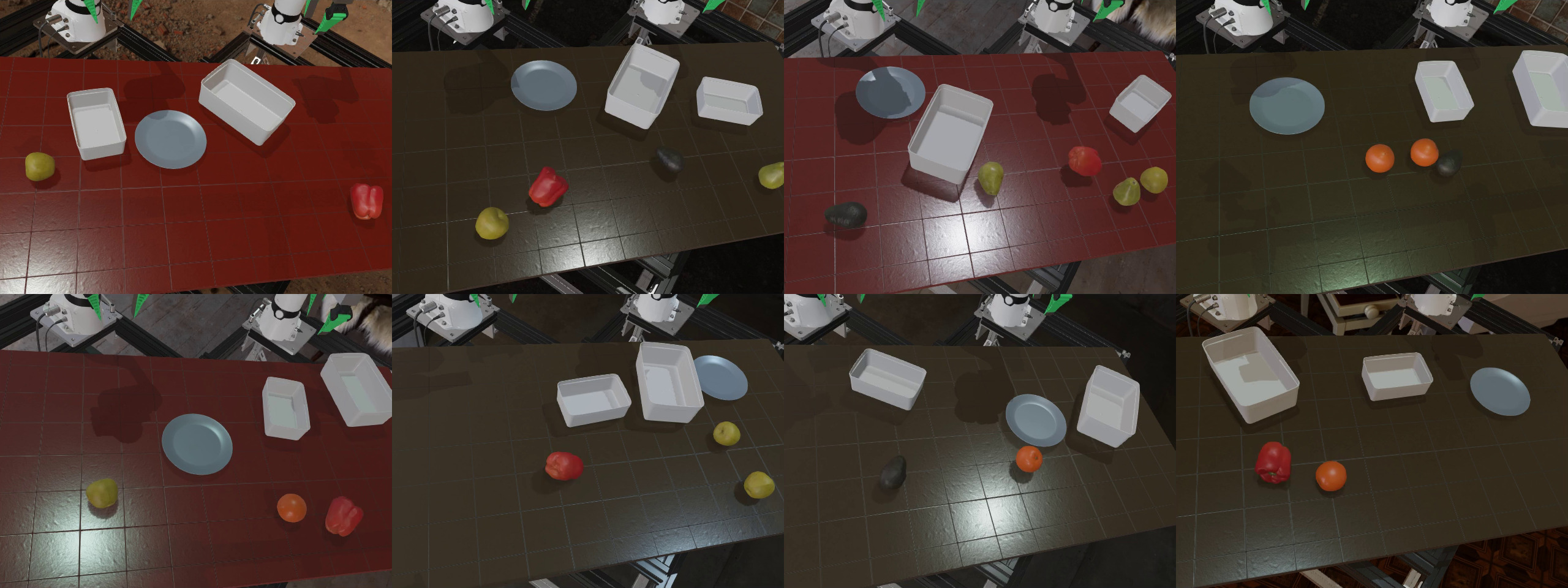
| Distribution Shift Type | Scenario S | Scenario D | Scenario B | Scenario K |
|---|---|---|---|---|
| distractor_textures | ✓ | ✓ | ||
| environment_map | ✓ | ✓ | ✓ | ✓ |
| lighting | ✓ | ✓ | ✓ | ✓ |
| table_top_texture | ✓ | ✓ | ||
| scene_extrinsics | ✓ | ✓ | ✓ | ✓ |
| scene_intrinsics | ✓ | ✓ | ✓ | ✓ |
| wrist_intrinsics | ✓ | ✓ | ✓ | ✓ |
8.3 Predicates
Five predicate tables specify progress for turning a container, nesting containers on a plate, covering fruit, sorting fruit/vegetables, and pouring vegetables. Dense state logs support temporal analysis beyond the final Boolean success flag. Some milestones explicitly reward intermediate rotations or the author’s intended strategy, so a different valid strategy need not receive identical partial credit.
| TurnLargeContainerUpsideDown |
|---|
| Robot’s right hand fingers touched the larger container |
| Robot’s left hand fingers touched the larger container |
| Robot turned the large container over 45 degrees |
| Robot turned the large container turn 90 degrees |
| Robot turned the large container turn 135 degrees |
| Robot flipped the large container upside down |
| PutContainersOnPlate |
|---|
| Robot lift the larger container |
| The large container on top of the plate |
| Robot lift the smaller container |
| The smaller container inside the larger container |
| PutFruitInLargeContainerAndCoverWithPlate |
|---|
| Robot picked up any fruit |
| Any fruit in the large container |
| Robot picked up the plate |
| All fruit in the large container and the plate on top of the large container |
| SeparateFruitsVegetablesIntoContainers |
|---|
| Robot picked up any fruit |
| Any fruit in the small container |
| Robot picked up any vegetable |
| Any vegetable in the large container |
| All fruit in the smaller container and all vegetable in the large container |
| DumpVegetablesFromSmallToLargeContainer |
|---|
| Robot picked up any vegetable |
| Robot put any vegetable in small container |
| Robot lifted the small container |
| Robot turned the small container over 45 degrees |
| Robot turned the small container over 90 degrees |
| Robot moved the small container over large container |
| Any vegetable inside the large container |
| All vegetable inside the large container while robot held the smaller container |
8.4 Missing simulation rollouts
Cloud execution or synchronization failures leave 104 missing rollouts across 39 of 238 task/policy/condition cells, about 0.2% of the planned simulation data. Table S4 lists the affected cells and actual counts. The analysis uses those available counts rather than treating every cell as exactly 200 trials.
| Task | Policy | Condition | Rollouts |
| Nominal conditions | |||
| PutBellPepperInBin | Single task | - | 199 |
| PutBellPepperInBin | LBM | Finetuned | 185 |
| PutSpatulaOnPlateFromRack | LBM | Pretrained | 199 |
| StackPlatesOnTableFromRack | LBM | Pretrained | 198 |
| StoreCerealBoxUnderShelf | Single task | - | 199 |
| PushCoasterToMug | Single task | - | 199 |
| PushCoasterToMug | LBM | Pretrained | 199 |
| SeparateFruitsVegIntoContainers | Single task | Trained with 15% data | 199 |
| PutFruitInLargeContainerAndCoverWithPlate | Single task | Trained with 50% data | 199 |
| Distribution shift | |||
| PutAppleFromBowlInBin | LBM | Pretrained | 198 |
| PutFruitFromBowlInBin | Single task | - | 199 |
| PutFruitFromBowlInBin | LBM | Pretrained | 198 |
| PutFruitFromBowlInBin | LBM | Finetuned | 198 |
| PutBellPepperInBin | Single task | - | 197 |
| PutBellPepperInBin | LBM | Pretrained | 193 |
| PutSpatulaOnPlateFromRack | Single task | - | 195 |
| PutSpatulaOnPlateFromRack | LBM | Pretrained | 197 |
| PutSpatulaOnPlateFromRack | LBM | Finetuned | 198 |
| StoreCerealBoxUnderShelf | Single task | - | 198 |
| PushCoasterToCenterOfTable | LBM | Pretrained | 198 |
| PushCoasterToMug | LBM | Pretrained | 198 |
| PushCoasterToMug | LBM | Finetuned | 199 |
| PutBananaOnSaucer | Single task | - | 199 |
| PutKiwiInCenterOfTable | Single task | - | 191 |
| TurnCupUpsideDown | LBM | Pretrained | 199 |
| PutContainersOnPlate | Single task | - | 199 |
| PutContainersOnPlate | Single task | Trained with 15% data | 199 |
| PutContainersOnPlate | LBM | Pretrained | 199 |
| PutFruitInLargeContainerAndCoverWithPlate | Single task | - | 198 |
| PutFruitInLargeContainerAndCoverWithPlate | Single task | Trained with 15% data | 199 |
| SeparateFruitsVegIntoContainers | Single task | - | 199 |
| SeparateFruitsVegIntoContainers | LBM | Pretrained | 199 |
| TurnLargeContainerUpsideDown | LBM | Finetuned with 50% data | 199 |
| BimanualPlaceAvocadoFromBowlIntoBin | Single task | - | 198 |
| Fractional pretraining | |||
| DumpVegetablesIntoContainer | LBM | TRI-Ramen-25 + FT@100 | 199 |
| DumpVegetablesIntoContainer | LBM | TRI-Ramen-50 + FT@15 | 199 |
| PutContainersOnPlate | LBM | TRI-Ramen + FT@100 | 198 |
| PutFruitInLargeContainerAndCoverWithPlate | LBM | TRI-Ramen-25 + FT@15 | 198 |
| SeparateFruitsVegIntoContainers | LBM | TRI-Ramen-50 + FT@50 | 199 |
9 Real-world evaluation details
The hardware supplement documents scene setup, termination decisions, task demonstrations, initial-condition examples, and the complete manually scored rubrics.
9.1 Real-world evaluation process
Overlaid camera views and homographic alignment help reproduce scenes across stations, but tall objects violate the planar approximation and occlusion can confuse operators. Many objects, deformables, food, and irreversible actions make resets especially laborious.
Operators terminate on success, unsafe behavior, or sustained lack of progress, rather than a single fixed elapsed-time cutoff. This gives hardware policies more chances to recover, including after an initially wrong task, and is a major confound in comparing absolute hardware and simulation success.
9.2 Real-world evaluation tasks
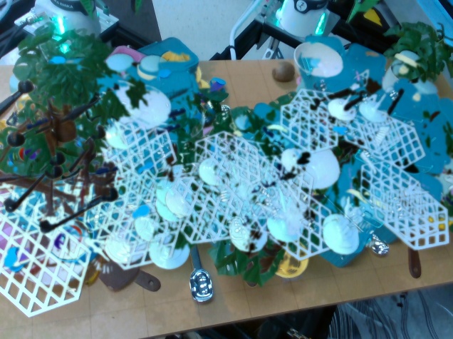
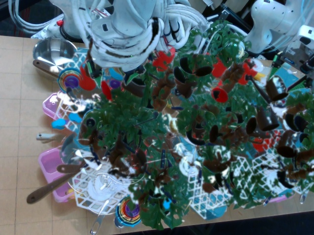
Successful film strips show precise bimanual rotor fitting, the multistage apple task lasting up to about three minutes, and ordered breakfast preparation. These illustrate what fine-tuned models can achieve; they are selected successful examples rather than estimates of reliability. Table S5 retains the task-specific demonstration counts and evaluation conditions.
| Experiment | Task | Nominal | Diff. Station | DS | wood_island | hersey | maverick | ruggles | salem | davis | milton | Total |
|---|---|---|---|---|---|---|---|---|---|---|---|---|
| Seen | PutKiwiInCenterOfTable | X | X | X | 0 | 0 | 0 | 0 | 49 | 0 | 0 | 49 |
| Seen | TurnMugRightsideUp | X | X | X | 0 | 121 | 0 | 0 | 122 | 122 | 125 | 490 |
| Seen | PushCoasterToMug | X | - | X | 98 | 0 | 0 | 0 | 98 | 0 | 0 | 196 |
| Unseen | ClearKitchenCounter | X | X | - | 0 | 0 | 0 | 0 | 0 | 305 | 0 | 305 |
| Unseen | BikeRotorInstall | X | - | - | 0 | 0 | 0 | 533 | 0 | 0 | 0 | 533 |
| Unseen | CutAppleInSlices | X | - | - | 496 | 0 | 0 | 0 | 0 | 0 | 0 | 496 |
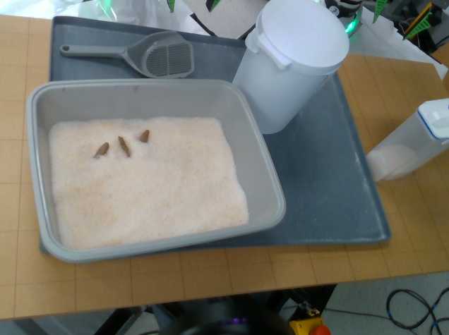
| Unseen | CleanLitterBox | X | - | - | 0 | 0 | 0 | 0 | 0 | 0 | 260 | 260 |
| Unseen | SetUpBreakfastTable | X | - | - | 0 | 229 | 0 | 0 | 0 | 0 | 0 | 229 |
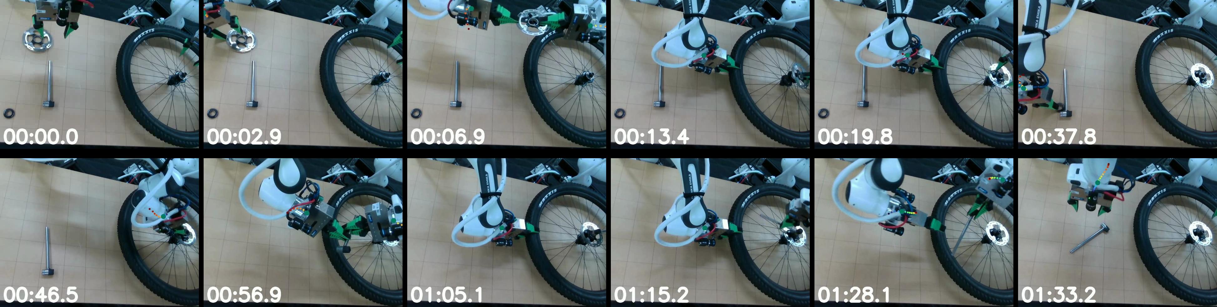
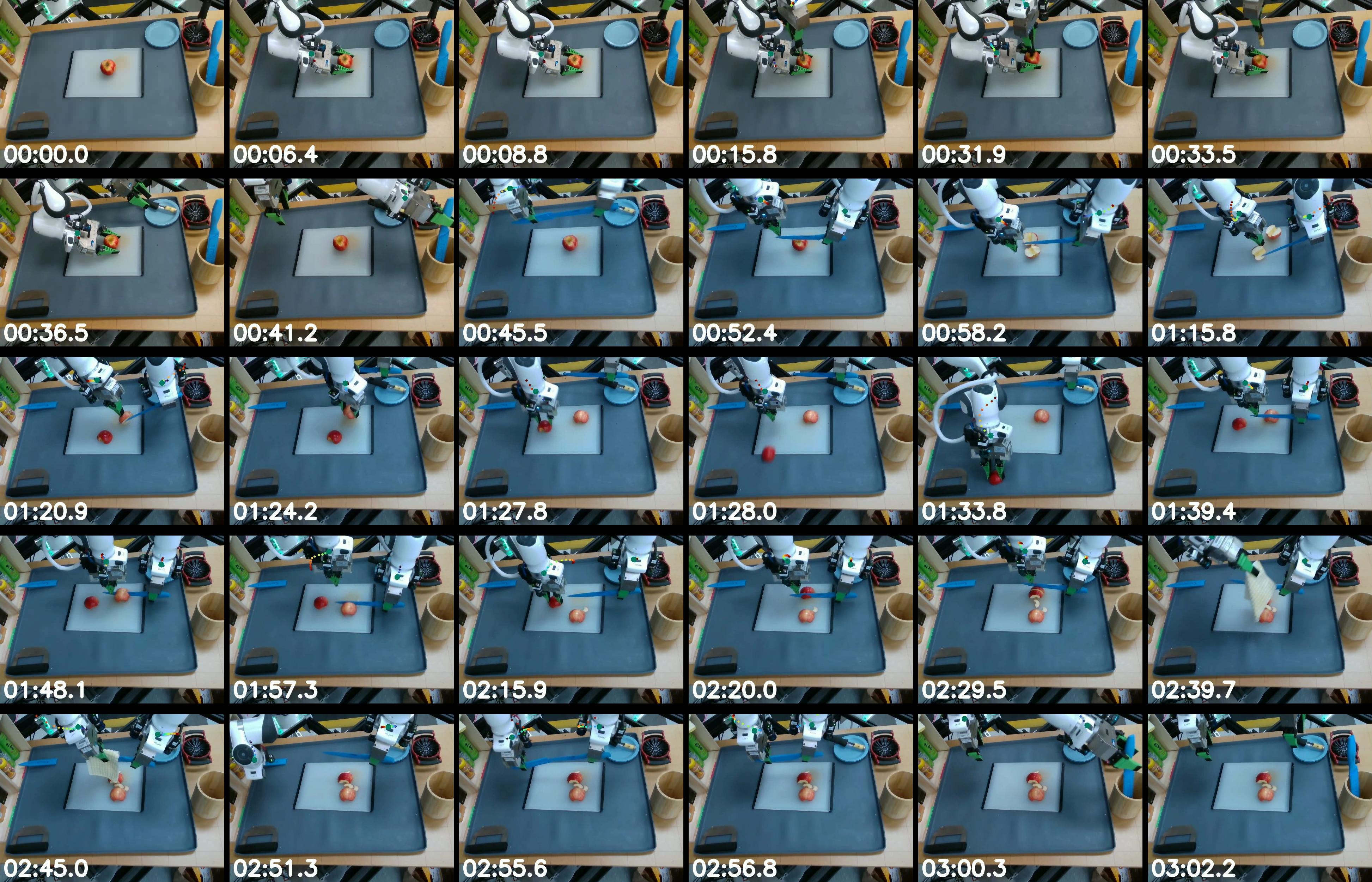
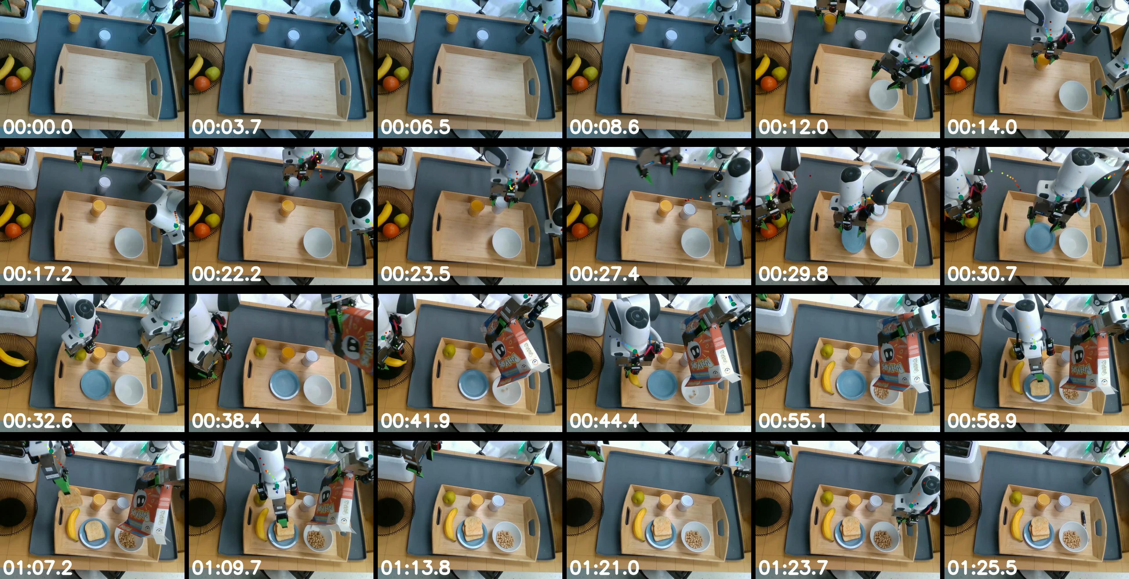
9.3 Sample real-world initial conditions
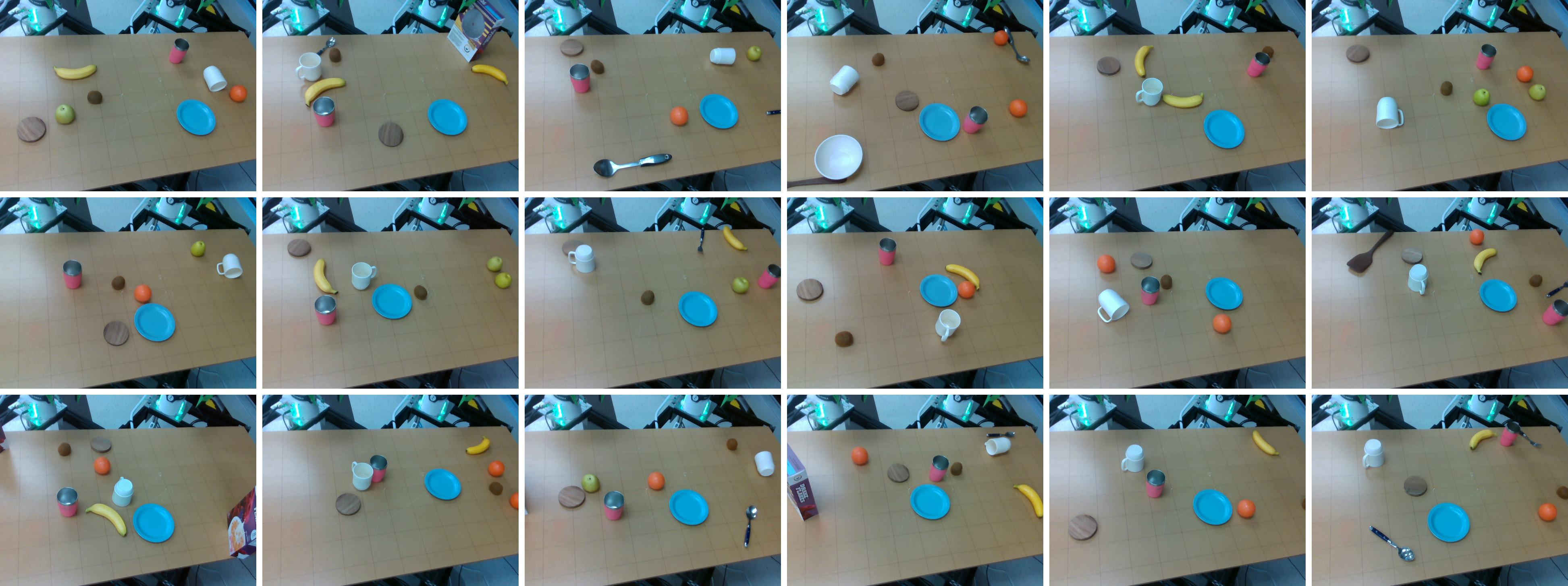
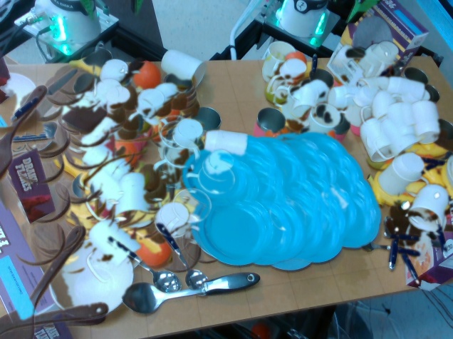
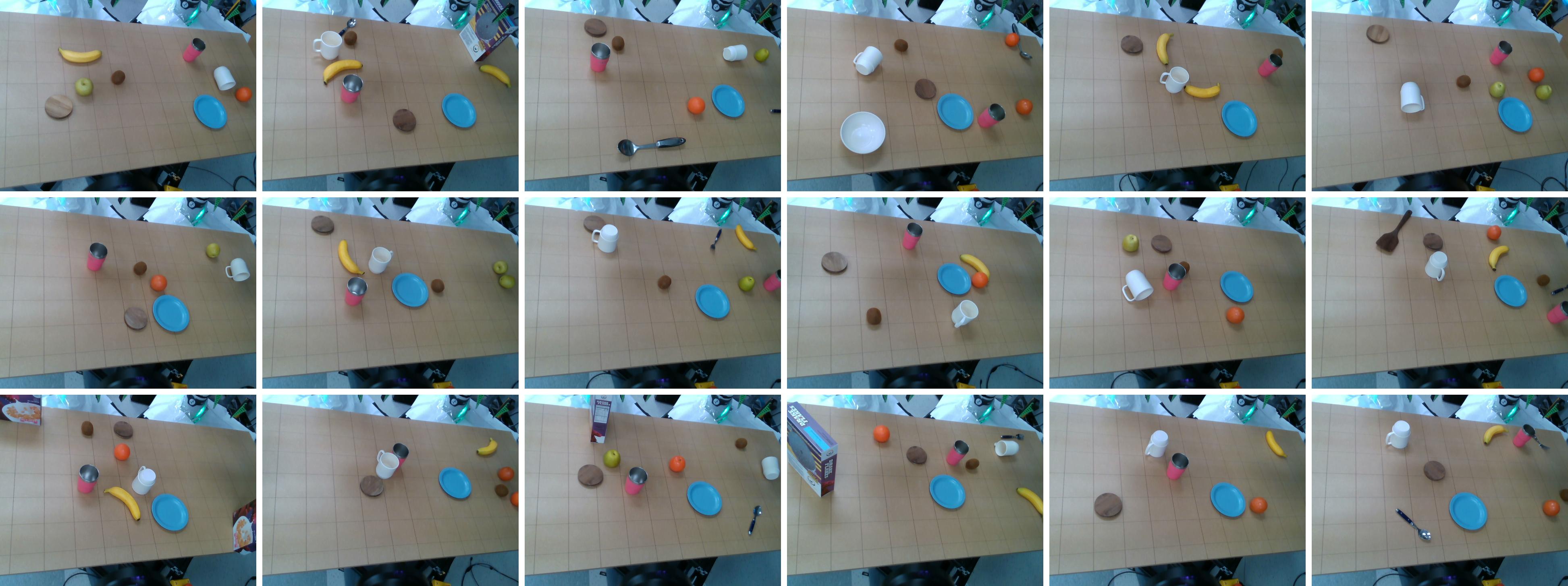
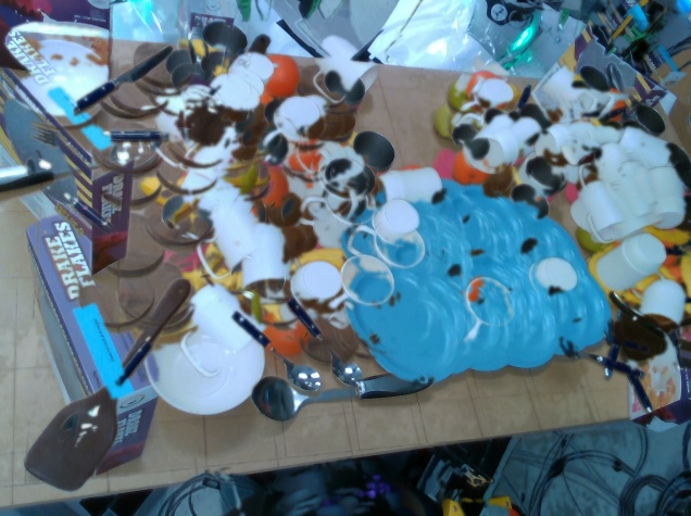
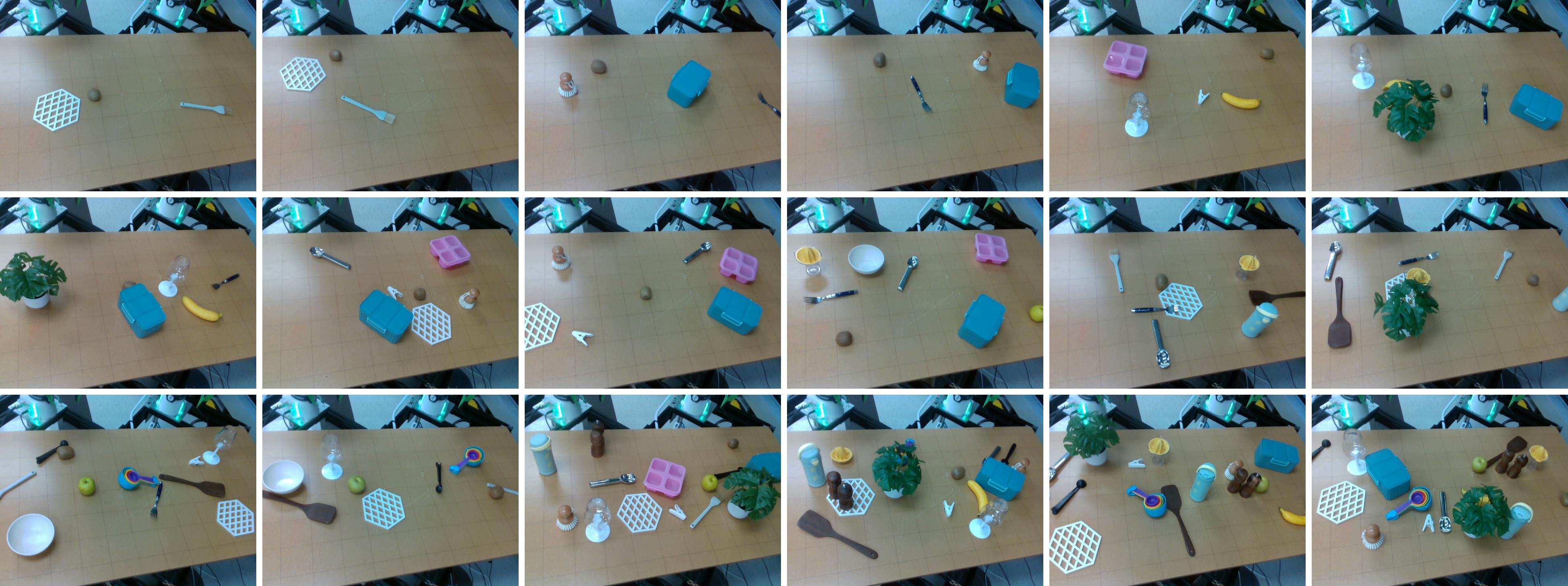
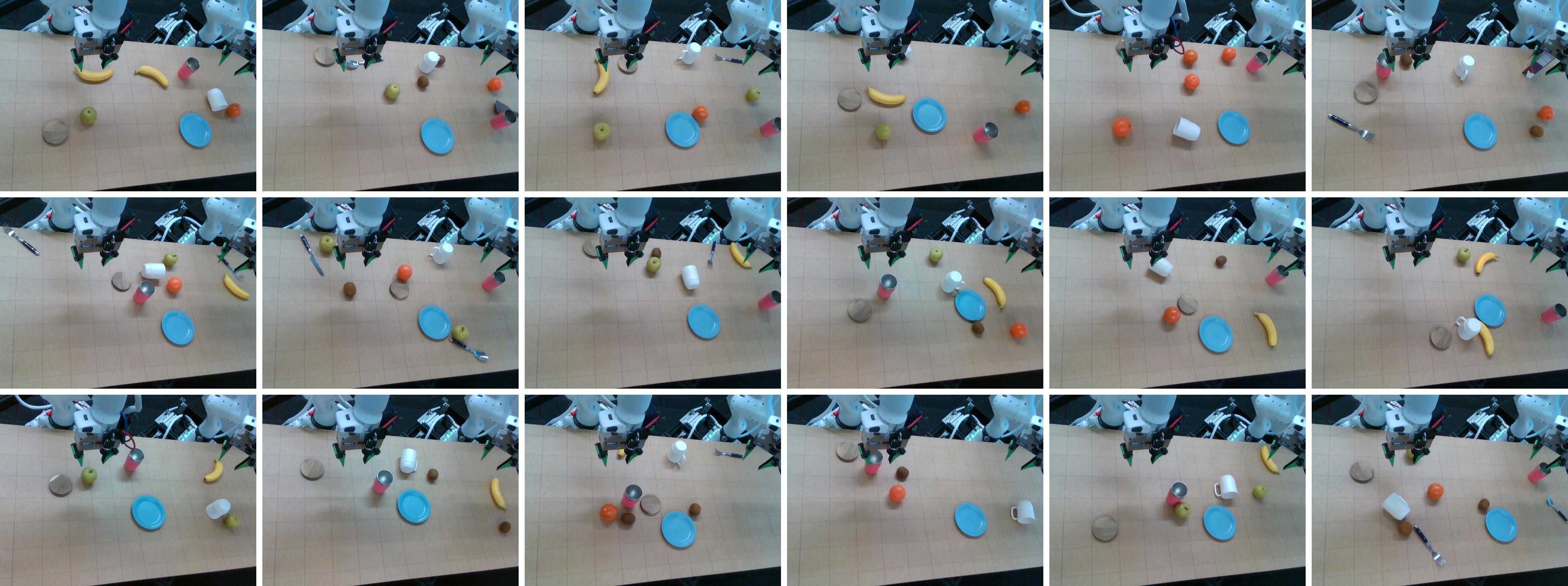
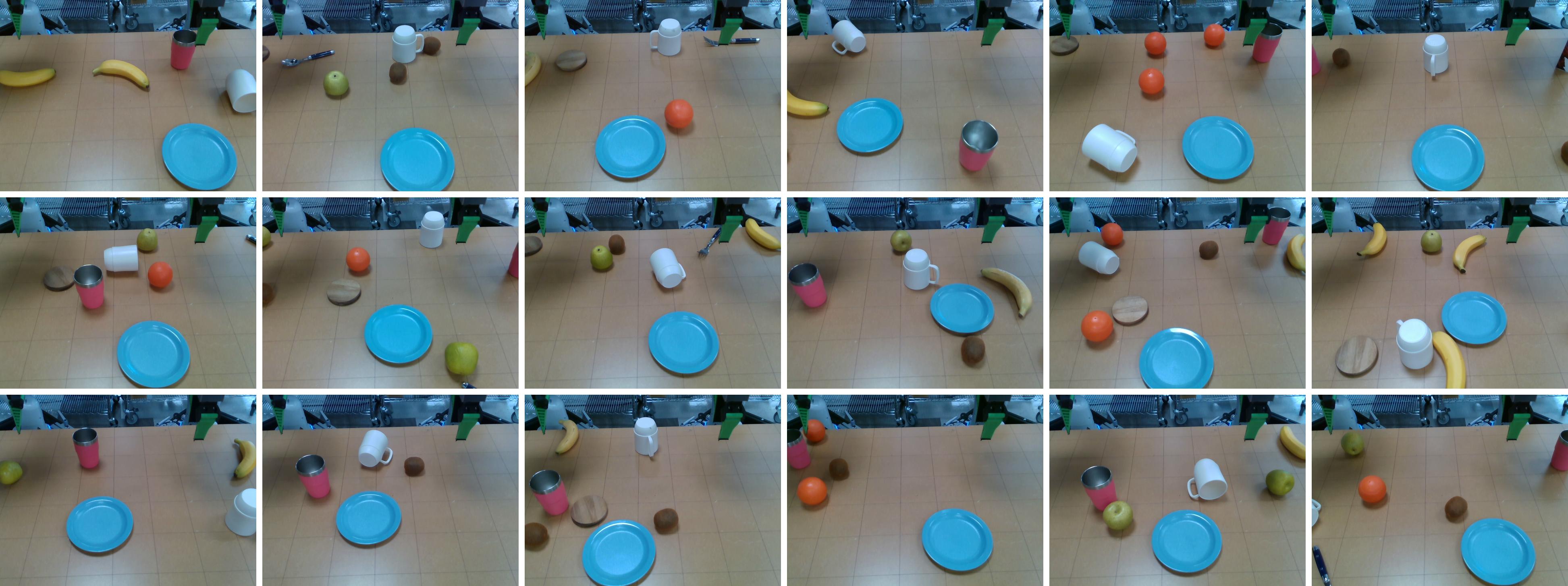
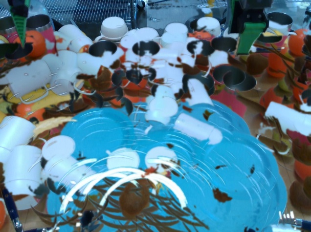
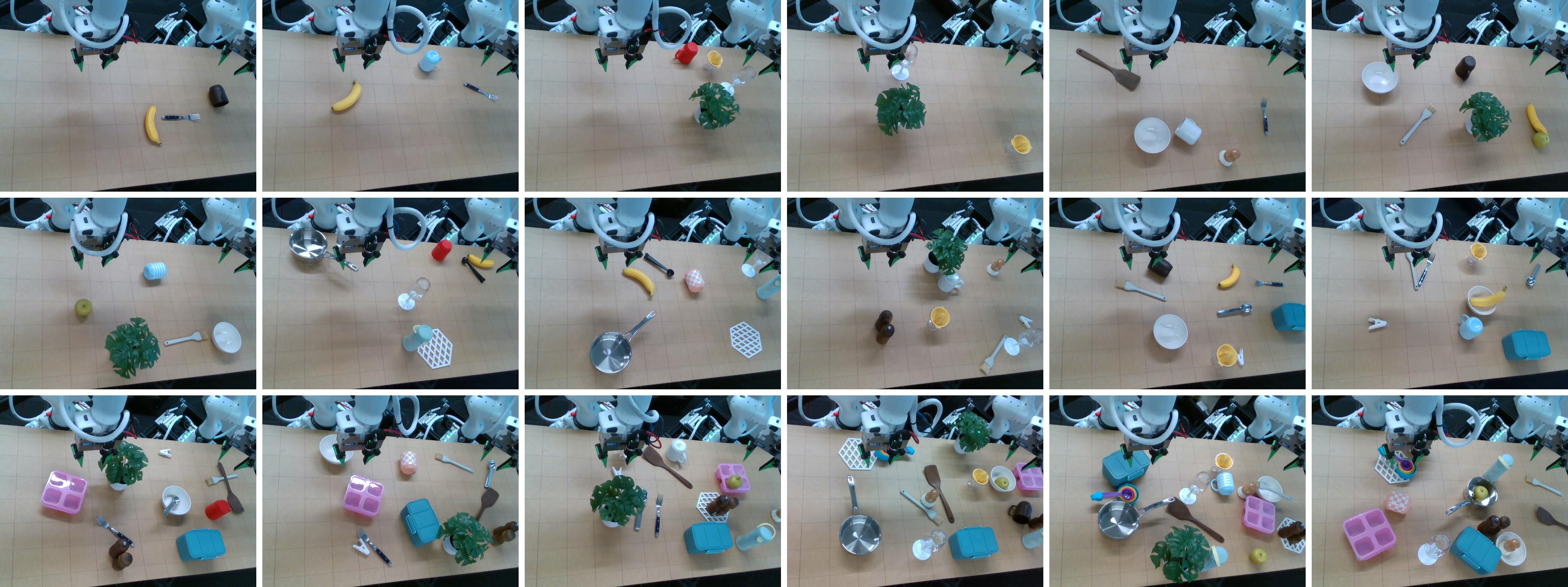
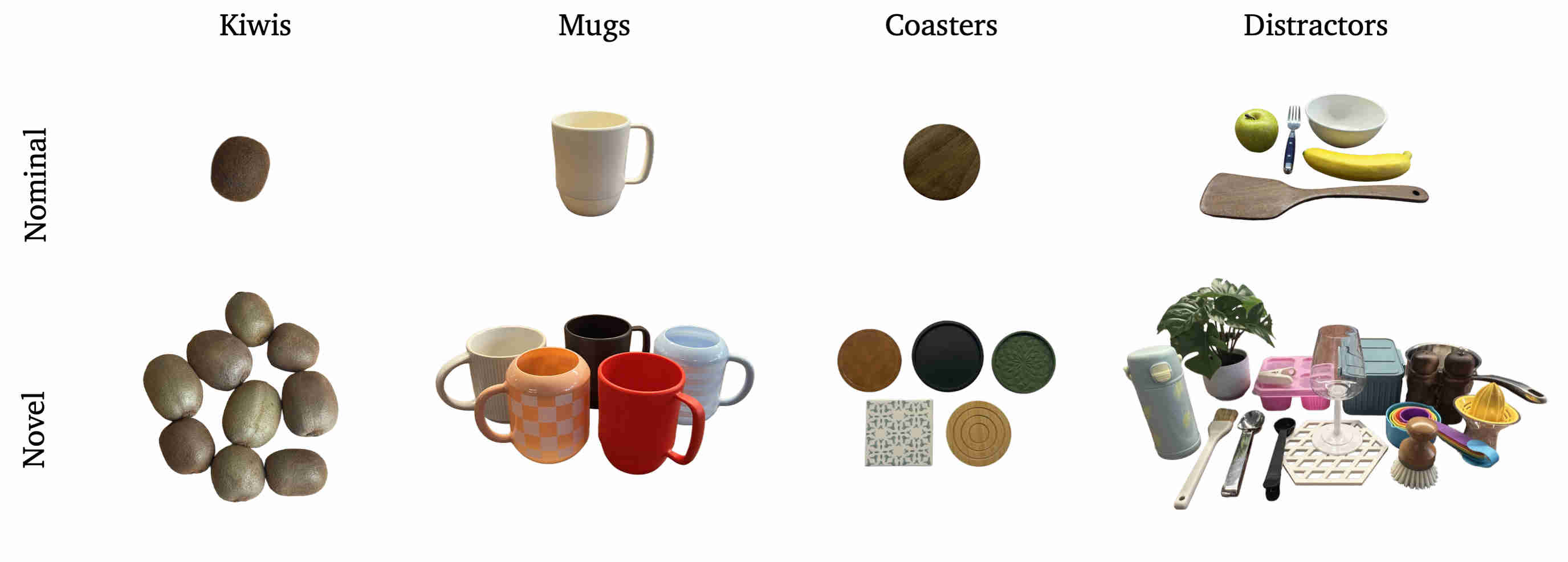
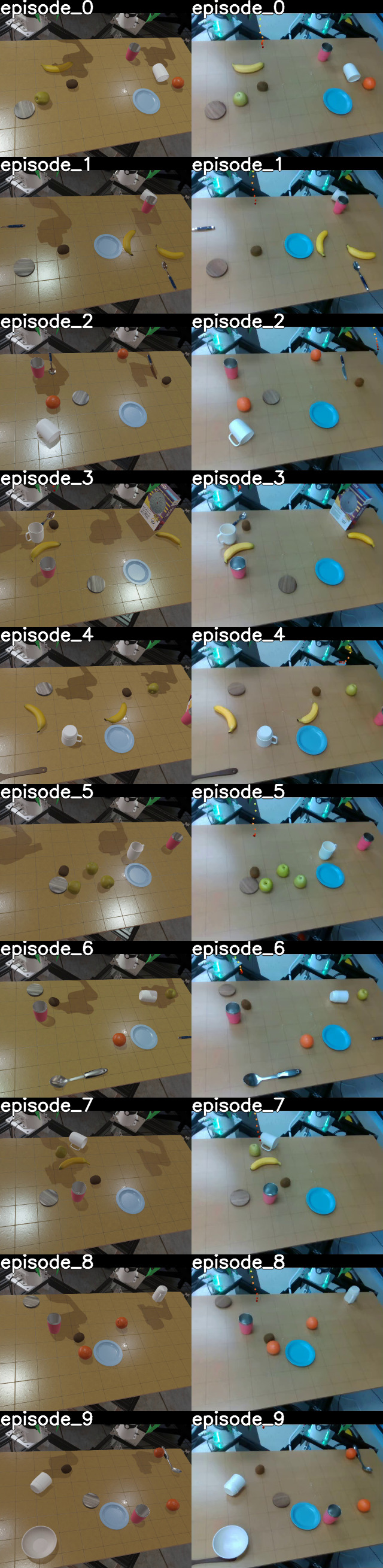
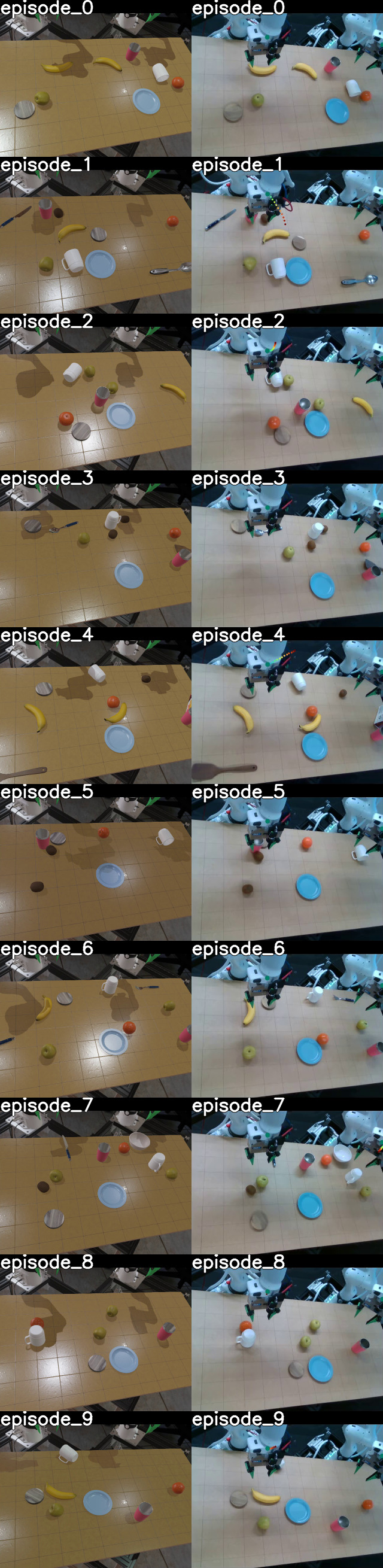
The supplement shows all eight hardware task setups and detailed nominal, station-transfer, and object-shift examples for kiwi placement and mug turning. Shape and appearance variation is larger for mugs and coasters than for kiwis. A different kiwi is sampled for each initial-condition bundle, illustrating that the intensity of shift varies by task.
9.4 Rubrics for real-world tasks
The five original yes/no rubric tables remain intact for counter cleanup, breakfast setup, rotor installation, apple slicing, and litter-box cleanup. They award milestone credit for intermediate handling and tool-use steps, so task-completion scores need not imply final task success or safe completion of every stage.
| BimanualClearKitchenCounter |
|---|
| Robot picked up and placed all tools in the tray receptacle |
| Robot picked up the sponge |
| Robot held the cutting board in place |
| Robot cleaned the cutting board with the sponge |
| Robot moved the cutting board aside to make room for cleaning |
| Robot swept the waste into the trash bin |
| Robot dropped the sponge and returned to the home position |
| BimanualSetUpBreakfastTable |
|---|
| Robot opened the cabinet door |
| Robot picked the bowl up and placed it on the tray |
| Robot placed the milk cup on the tray |
| Robot placed the juice cup on the tray |
| Are the milk and juice cups upright? |
| Robot placed the plate on the tray |
| Robot put the apple on the tray |
| Robot put the banana on the tray |
| Robot picked up at least one toast from the toaster |
| Robot put the toast on the plate |
| Robot poured the cereal into the bowl |
| Robot put the spoon on the tray |
| BimanualBikeRotorInstall |
|---|
| Robot picked up rotor |
| Robot handed over the rotor to other arm |
| Robot placed the rotor on the bike wheel |
| Robot seated the rotor onto the bike wheel |
| Robot picked up the lockring |
| Robot placed the lockring over the rotor |
| Robot handed over the tool to other arm |
| Robot placed the tool onto lockring |
| Robot positioned the tool into lockring grooves |
| Robot tightened the lockring at least one revolution |
| Robot engaged the threads of the lockring |
| Robot took off the tool from the lockring |
| Robot puts the tool back onto the table |
| CutAppleInSlices |
|---|
| Robot grasped the apple |
| Robot grabed the corer and aligned it with apple center |
| Robot cored the apple successfully |
| Robot unsheathed the knife and aligned it with the center of the apple |
| Robot sliced the apple into two halves |
| Robot fliped one half of apple |
| Robot fliped the other half of apple |
| Robot sliced one half of the apple in at least 3 slices |
| Robot picked up the cloth |
| Robot wiped the knife |
| Robot placed the cloth on top of the shelf |
| Robot picked up the knife sheath |
| Robot sheathed the knife |
| Robot placed the knife into the utensil crock |
| CleanLitterBox |
|---|
| Robot grasped the cat litter scoop |
| Robot scooped up the cat excrement |
| Robot used the other arm to open the trash can |
| Robot poured the cat excrement into the trash can |
| Robot repeated scooping until all excrement is removed from the litter box |
| Robot closed the trash can |
| Robot placed the scoop back onto the table |
10 “Seen” tasks under nominal conditions analysis: Breakfast Scenario
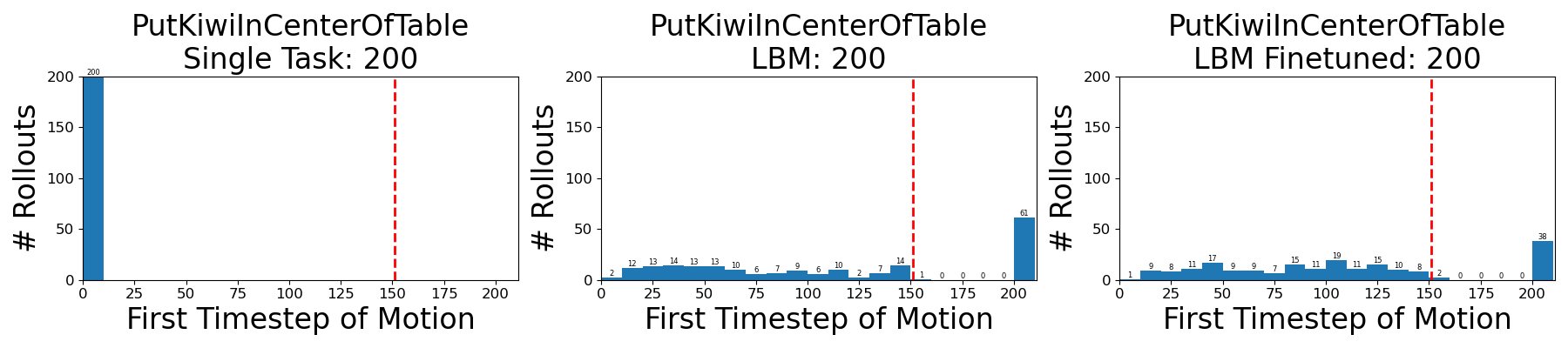
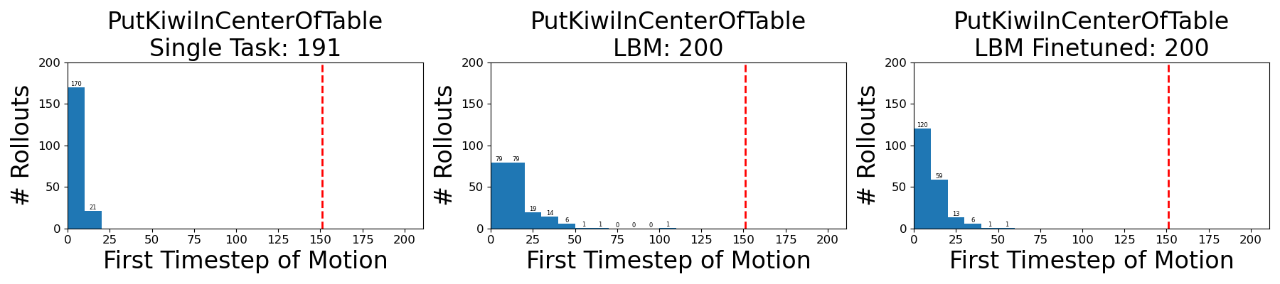
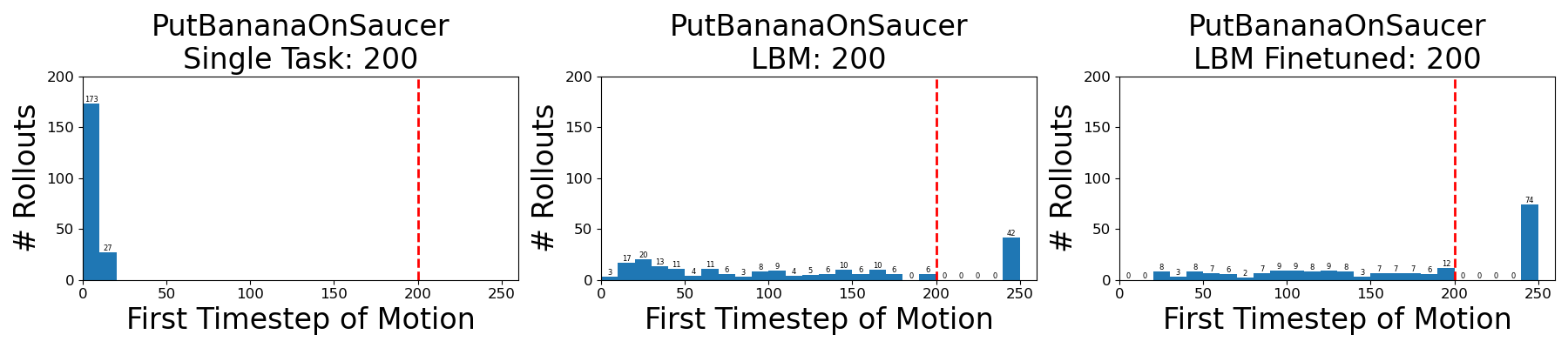
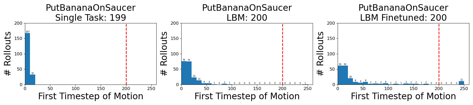
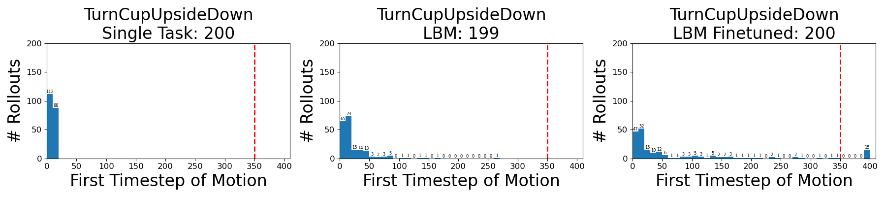
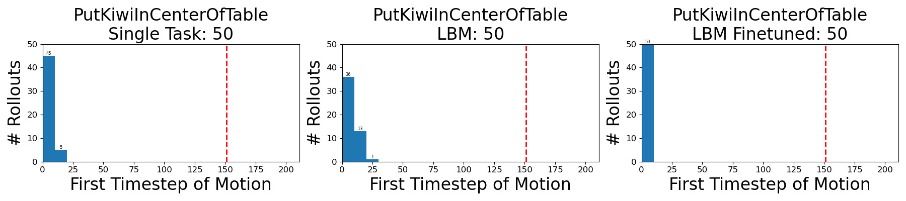
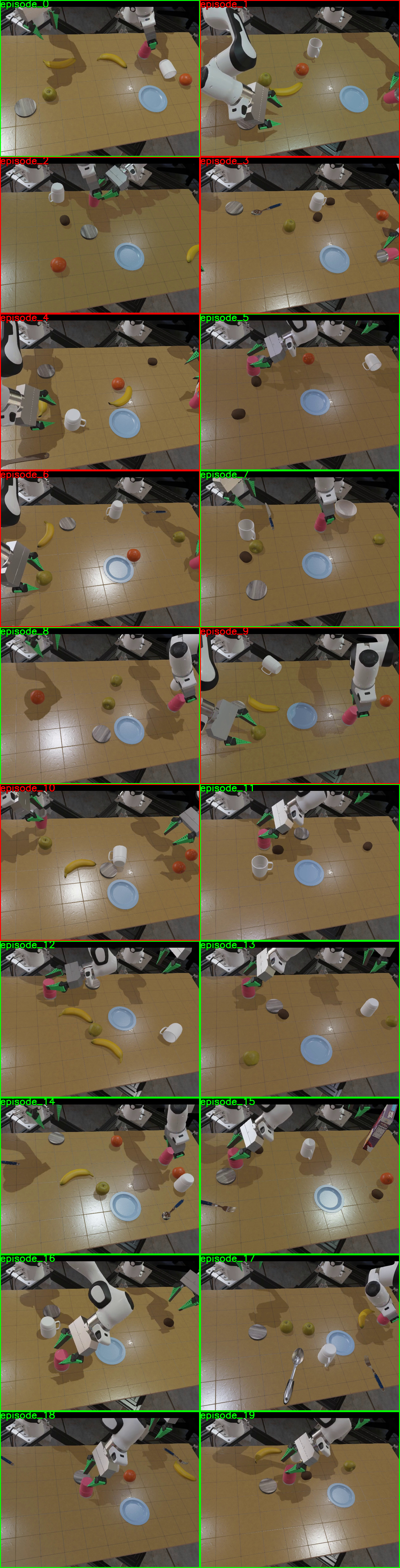
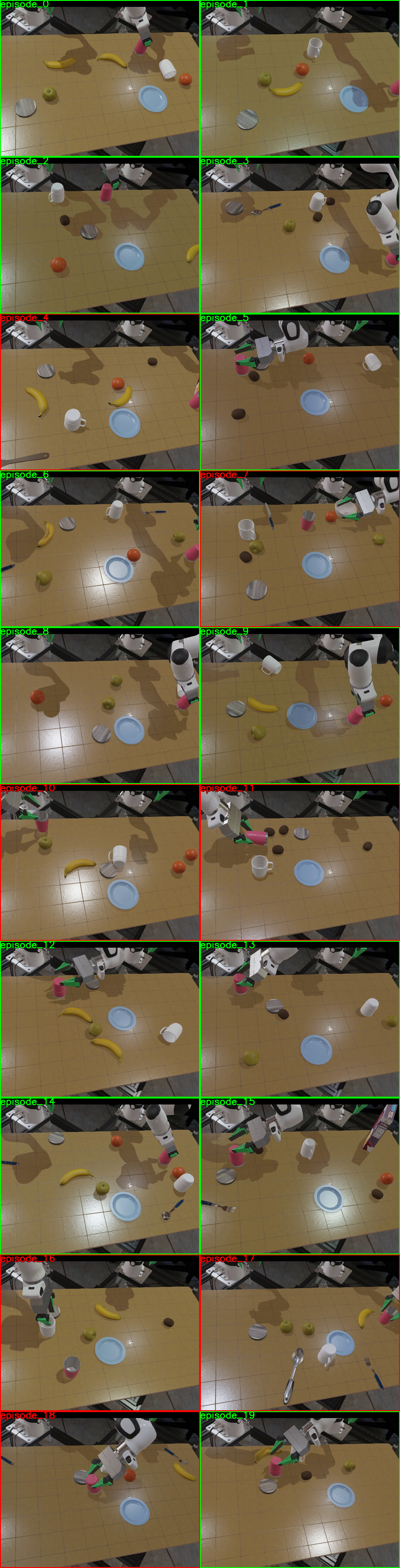
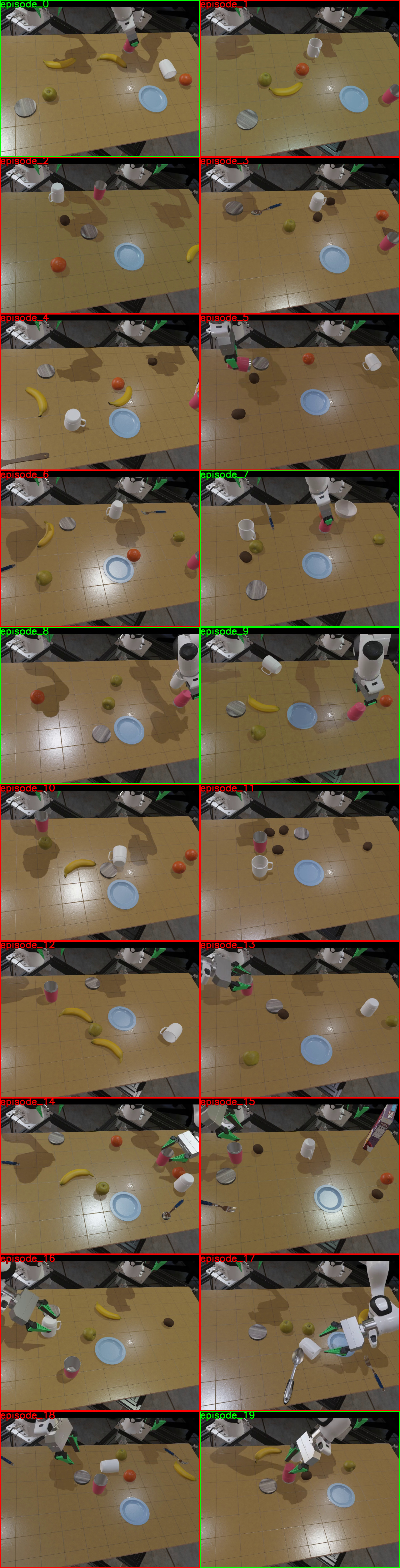
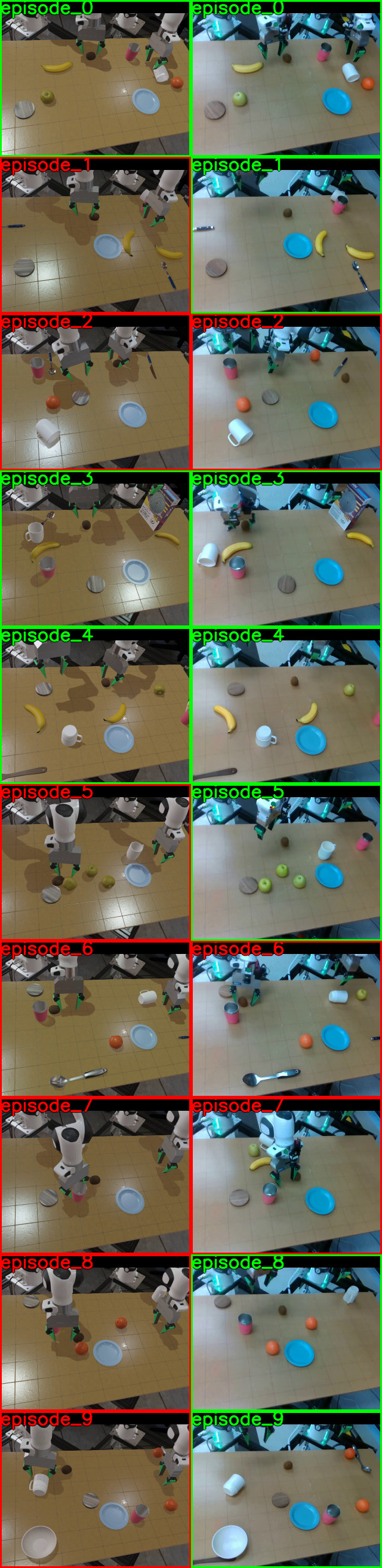
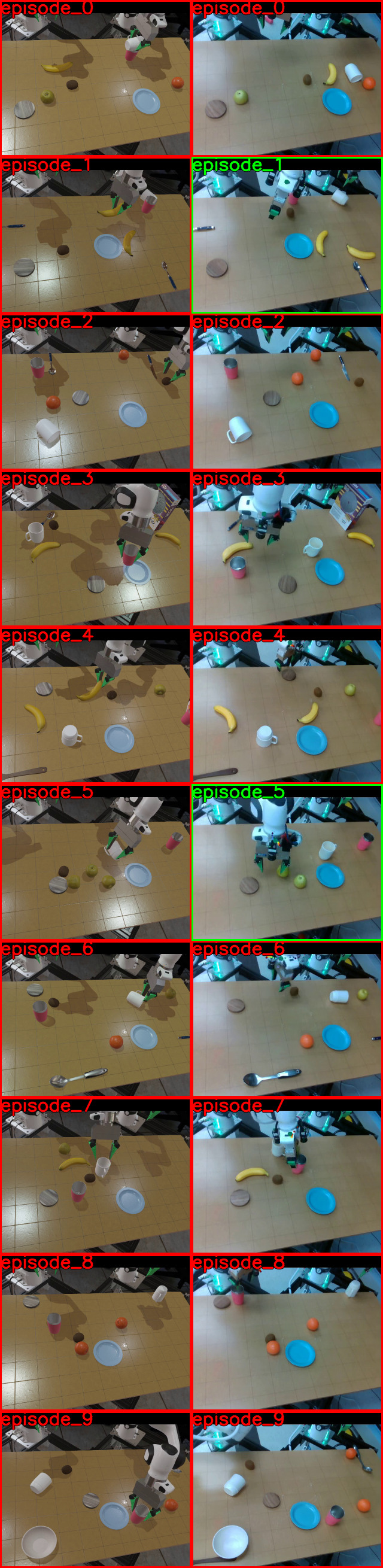
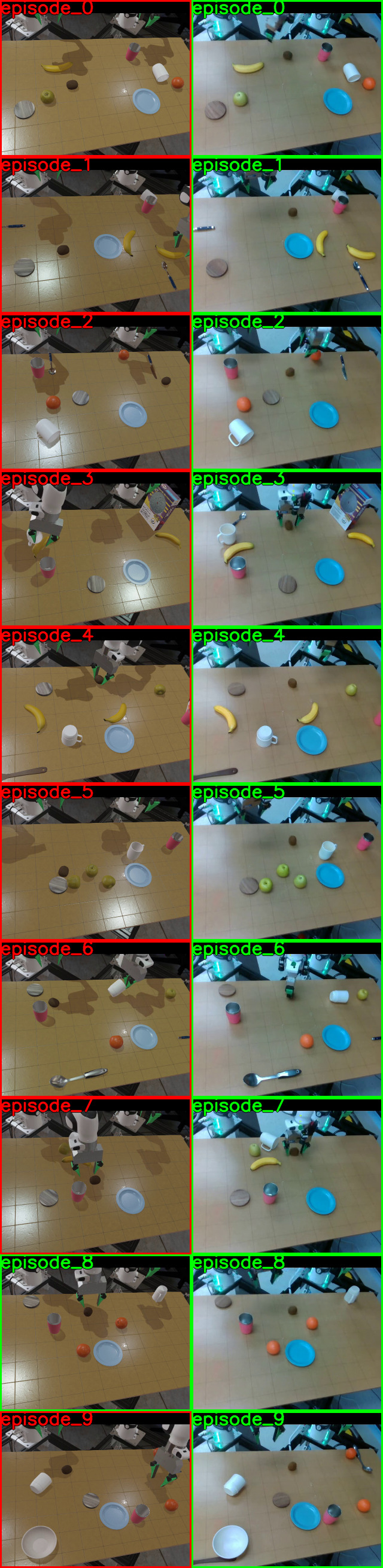
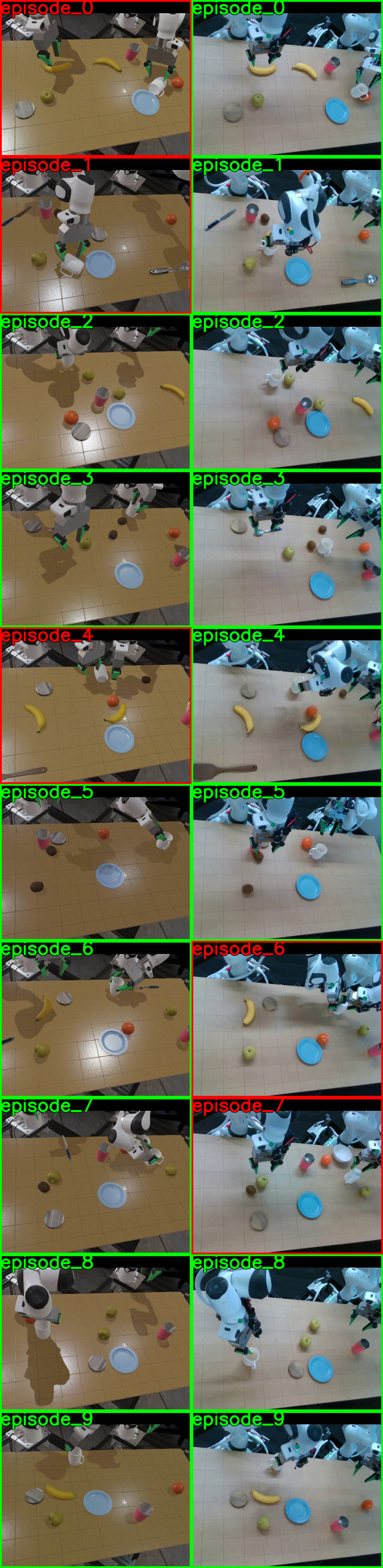
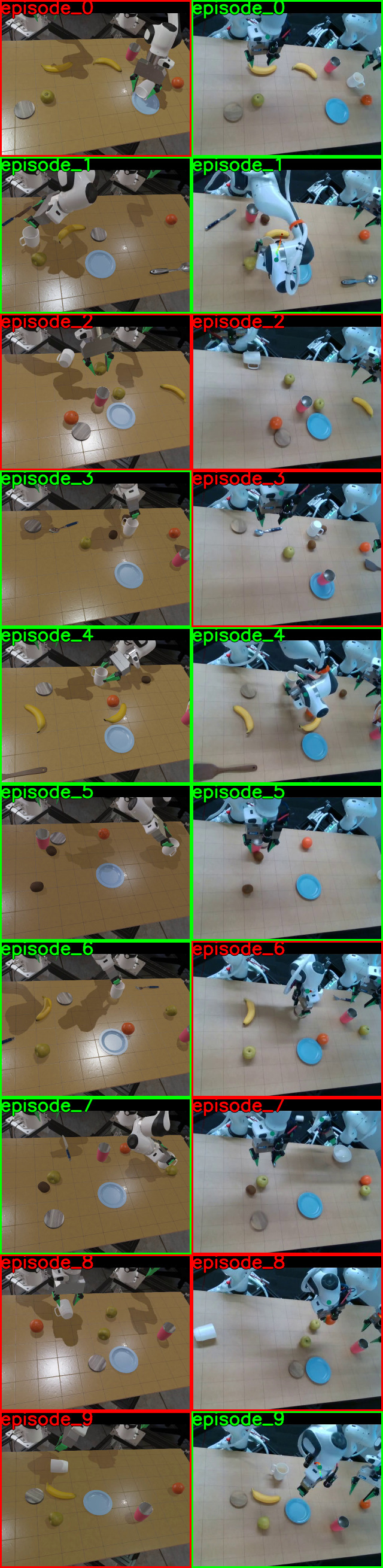
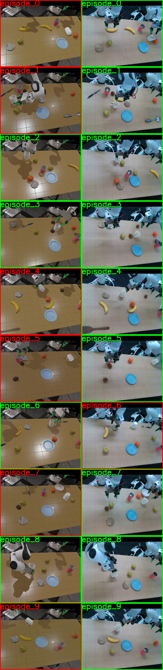
The Breakfast analysis links sparse demonstrations, wrong-task execution, and delayed motion to performance failures. Terminal-frame montages show what was manipulated, while first-motion histograms distinguish incorrect action from inactivity. Demonstration count correlates with performance here but is not independently randomized from task difficulty.
10.1 PutKiwiInCenterOfTable and PutBananaOnSaucer
For kiwi placement and banana-on-saucer tasks, single-task models usually pursue the requested object but often fail at grasping or placement. Multitask models also manipulate unrelated objects or remain at the starting pose. Fine-tuning reduces some of these errors without eliminating them; all original terminal-frame examples are retained.
10.2 TurnCupUpsideDown
The cup-turning fine-tuned model performs worse because many trials never initiate motion. The pretrained model sometimes executes another task, while the single-task model’s more common failure is grasping. Filtering experiments later examine this specific inactivity problem.
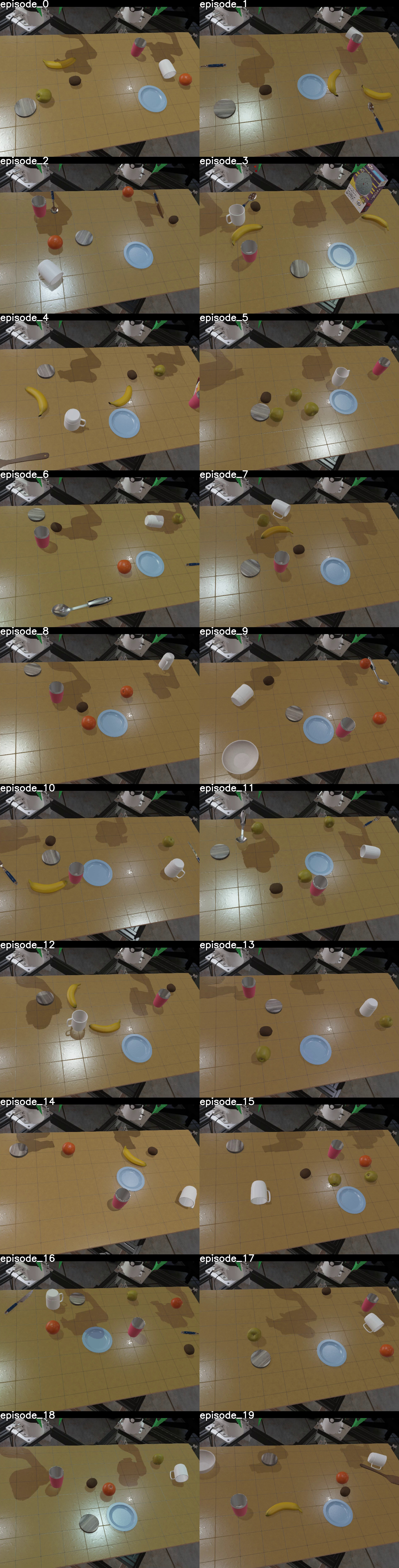
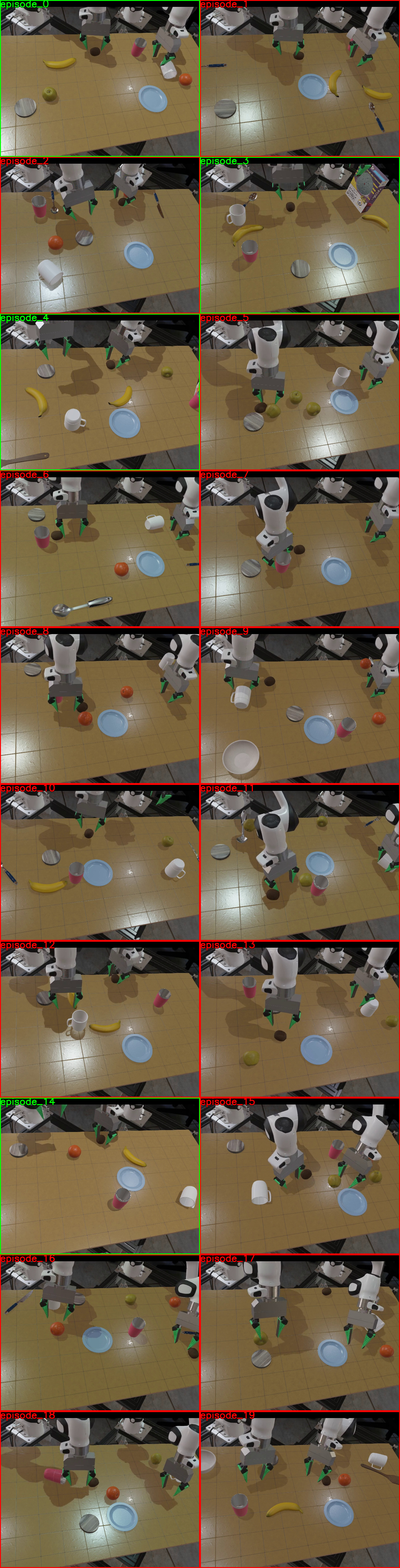
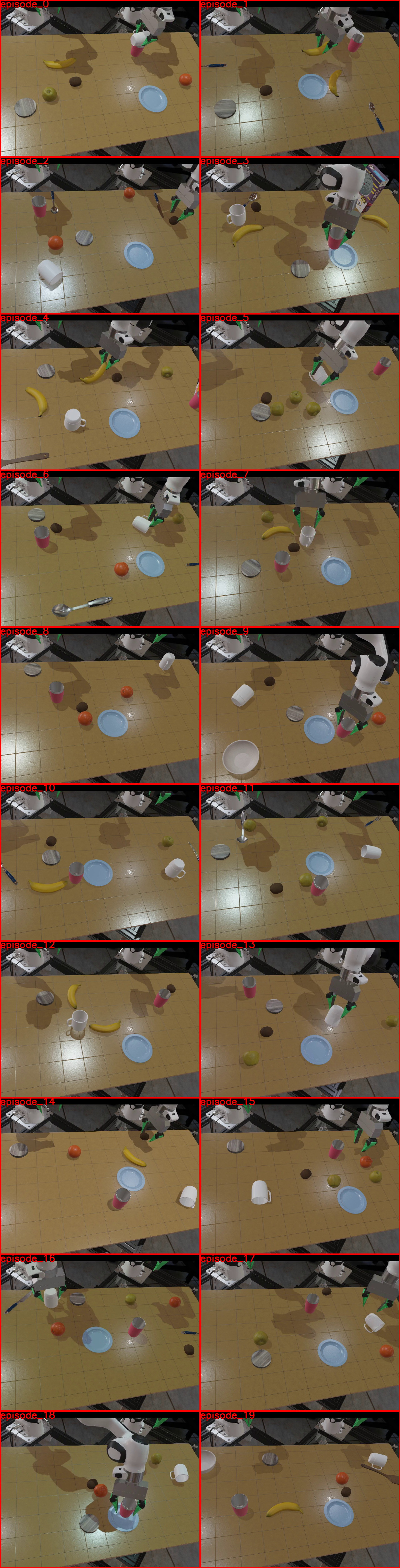
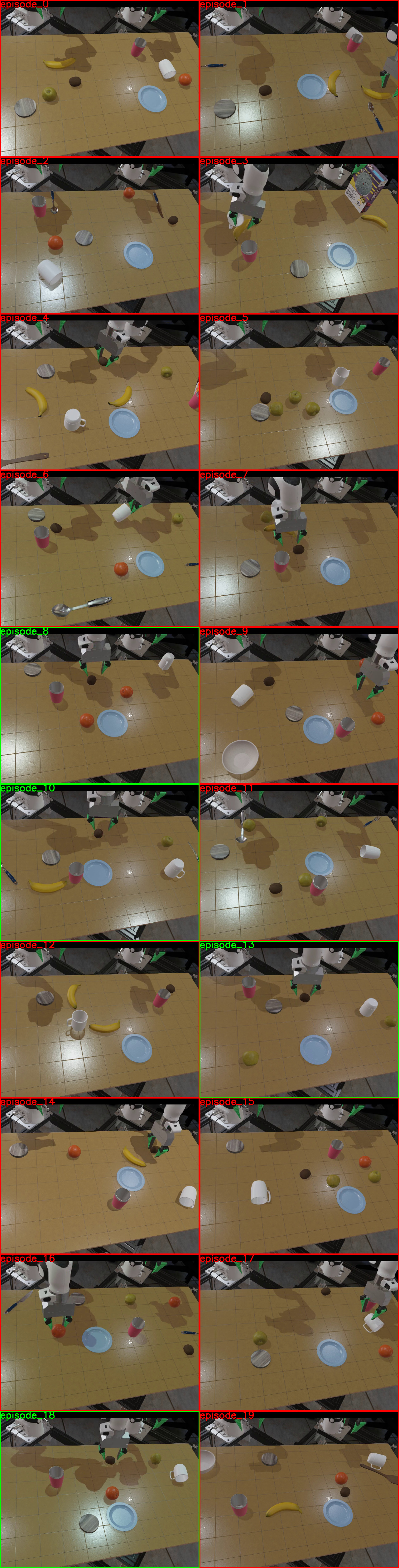
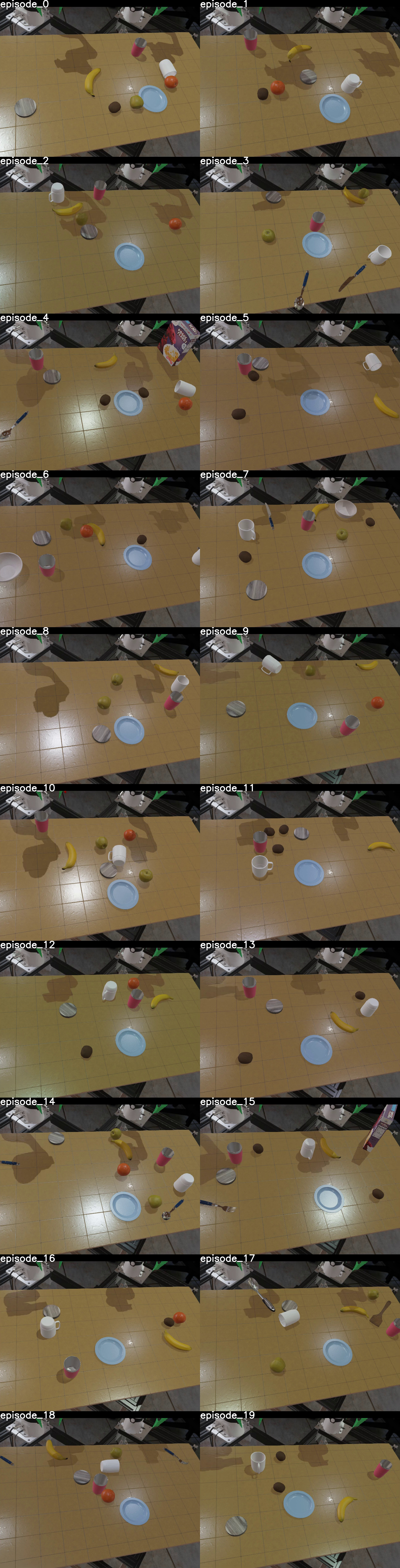
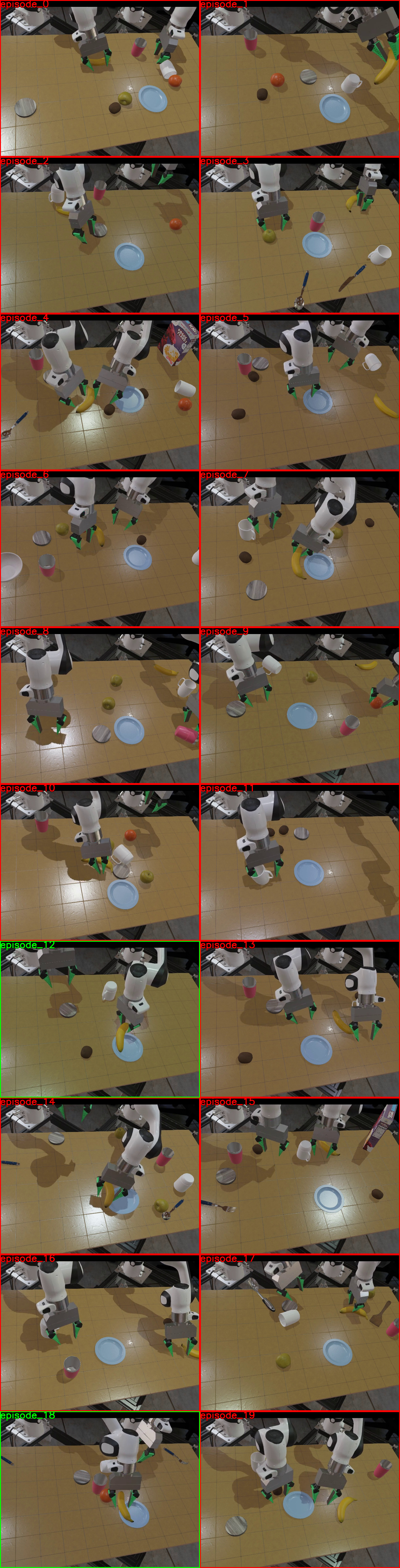
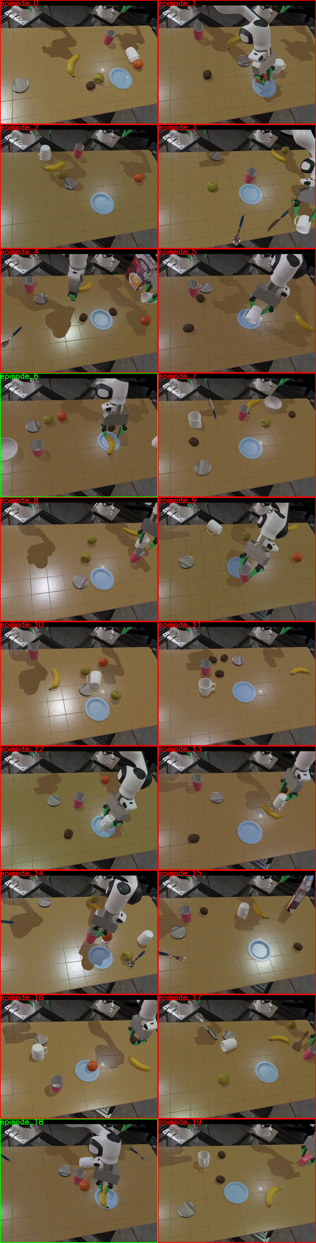
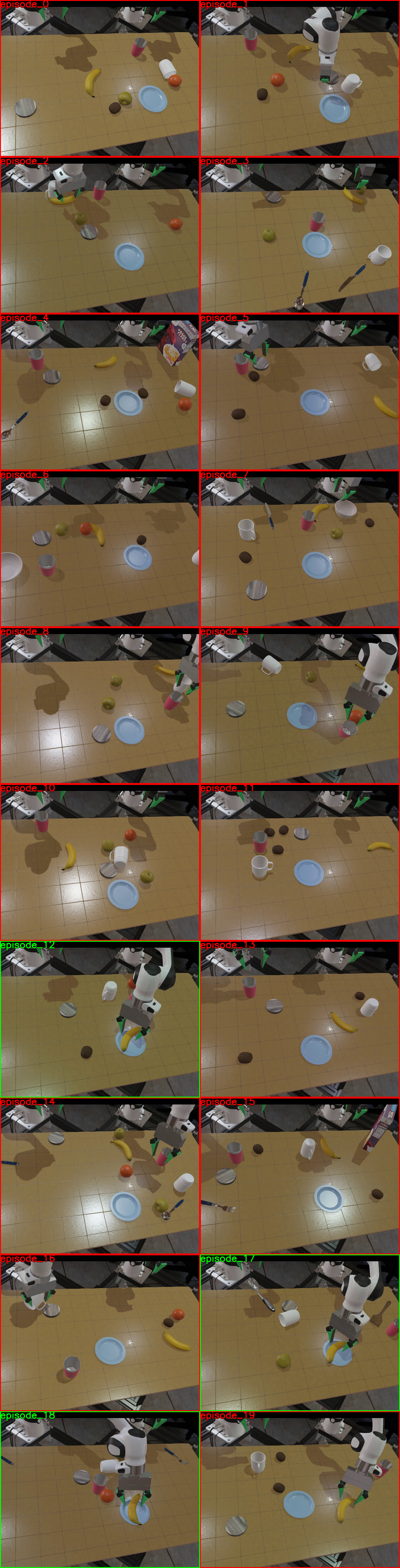
10.3 Simulation and Real Comparison for PutKiwiInCenterOfTable, TurnMugRightsideUp
Applying simulation timeouts to hardware trials reduces the fine-tuned mug model from 88% success to 50%, close to its 46.5% simulation result. Kiwi placement remains discrepant: 82% physical success becomes 70% under the cutoff, versus 9% in simulation. Thus timing explains much of one gap but not both. The same pretrained model also pauses more in simulation, suggesting additional domain-dependent behavior.
| Task x Policy | Sim | Real | Real w. |
| Sim Timeout | |||
| PutKiwiInCenterOfTable x single task | 0.135 | 0.44 | 0.2 |
| PutKiwiInCenterOfTable x LBM pretrained | 0.02 | 0.2 | 0.04 |
| PutKiwiInCenterOfTable x LBM finetuned | 0.09 | 0.82 | 0.7 |
| TurnMugRightsideUp x single task | 0.375 | 0.84 | 0.46 |
| TurnMugRightsideUp x LBM pretrained | 0.485 | 0.56 | 0.28 |
| TurnMugRightsideUp x LBM finetuned | 0.465 | 0.88 | 0.5 |
11 Bayesian analysis for task completion
Figures S17 and S18 replot the same completion data as posterior uncertainty in the mean, complementing the full rollout distributions in the main figures. They add a statistical view, not another set of independent experiments.
12 Effects of dataset filtering
Filtering removes 3.3% of internal hardware data and 11.7% of internal simulation data. Models initiate actions sooner, but filtered pretraining worsens language steering in the unadapted policy. Fine-tuned aggregate performance is similar, with substantial gains on particular tasks previously dominated by inactivity.
The authors hypothesize that idle initial frames emphasize instruction learning because these scenes are visually ambiguous. That mechanism is a hypothesis, not a separately isolated causal result. The same severe initiation delays were not observed on hardware, and the full filtering study is simulation-only.


13 Additional pretraining dataset details
Table S7 gives unnormalized sampling weights summing to 1.045. Internal real, simulated, and handheld sources receive weights 0.5, 0.25, and 0.05 before normalization; public sources share the remainder. Consequently roughly 76.6% of training samples come from internal sources by these weights, despite public datasets providing most raw hours.
| Data source name | Weights |
|---|---|
| lbm_real | 0.5 |
| lbm_sim | 0.25 |
| lbm_umi | 0.05 |
| bc_z | 0.03 |
| berkeley_autolab_ur5 | 0.007 |
| bridge_data_v2 | 0.02 |
| droid | 0.05 |
| fractal20220817_data | 0.03 |
| furniture_bench_dataset_converted_externally_to_rlds | 0.02 |
| jaco_play | 0.005 |
| language_table | 0.015 |
| nyu_franka_play_dataset_converted_externally_to_rlds | 0.05 |
| stanford_hydra_dataset_converted_externally_to_rlds | 0.01 |
| utokyo_xarm_pick_and_place_converted_externally_to_rlds | 0.003 |
| viola | 0.005 |
| Total weight | 1.045 |
14 Data normalization experiment
The corrected normalizer is tested on seen simulation tasks. It produces no clear aggregate nominal gain but improves shifted-condition performance on four of 16 tasks and in aggregate. This restricted follow-up supports sensitivity to normalization; it does not replace the original bug-affected main experiments or establish corrected hardware performance.