This essay argues that world models should support action-conditioned simulation for reasoning, planning, and agent learning. It organizes the design problem around data, representation, architecture, training objectives, and usage.
Its proposed GLP architecture combines discrete concepts, continuous perceptual features, and observation reconstruction. PAN sketches how those components might support hierarchical agents. This paper presents a position and architectural proposal, not a controlled benchmark demonstrating general intelligence. Some stated theoretical guarantees require stronger assumptions, identified below.
1 Introduction
The motivating idea is to compare imagined futures before acting. A useful world model should predict consequences across physical, social, and abstract situations, rather than merely generate plausible imagery. The authors advocate multimodal experience, mixed representations, hierarchical prediction, observation-grounded training, and policy learning from simulated experience.
This edition follows arXiv v5, revised June 2026; its publication date records the first preprint posting. Detailed PAN experiments belong to the separately cited companion paper. [66]
Equation 1
(1)
2 World Model and Agent Decision-Making
The formal setup pairs an agent’s action policy with an environment transition model and a goal-dependent reward. A learned world model supplies a usable surrogate when real interaction or exact dynamics are unavailable.
2.1 Agent-Environment Model and Optimal Agent
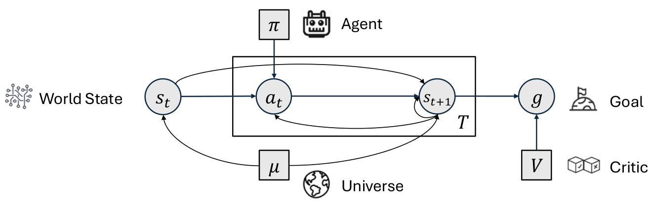
The paper writes trajectory probability as a product of action and environment-transition probabilities. Expected discounted reward defines a value function and motivates selecting actions by predicted future return. This idealized presentation assumes access to a sufficient state representation and a well-defined discounted objective.
Figure 1: A possible definition of an optimal agentEquations 2–5
(2)
(3)
(4)
(5)
2.2 World Model and Simulative Reasoning
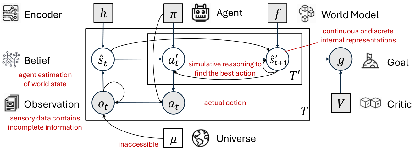
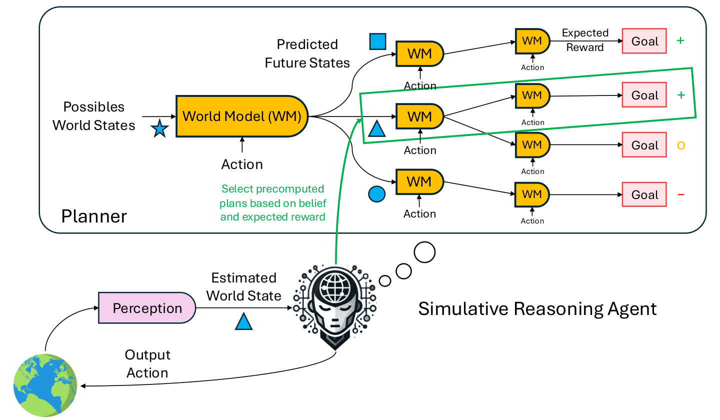
A practical agent encodes observations into an internal belief state, proposes actions, and rolls the world model forward. A critic evaluates those simulated futures. The authors emphasize persistent memory, multiple time scales, counterfactuals, and domains beyond physical motion.
These are desired capabilities of a general system. A learned simulator’s predictions and policy quality remain limited by its data, state representation, model error, and planning procedure.
Figure 2: An agent in real world where groundtruth world state and universe are unavailable to experience or experiment, so world model is crucial for simulation.Equation 6
(6)
3 The World Model Landscape
The survey groups contemporary systems by their main demonstrated capabilities. Its assessments reflect the essay’s cited versions and the authors’ preferred definition of a decision-oriented world model.
Gaming World Models
Game simulators produce action-conditioned visual trajectories, but the authors question their action diversity, interacting-agent support, and long-term consistency. These are scope limitations of the surveyed demonstrations, not a shared impossibility result.
Scene generators create explorable geometry. The essay distinguishes generating a static environment from learning its interactive dynamics, especially when exported geometry relies on a separate programmed physics engine.
Physical World Models
Driving and robotics world models learn useful physical regularities in specific domains. The critique asks whether their sensor interfaces, action spaces, and training distributions can support broader social or multi-agent situations.
Video Generation Models
Prompted video generation can depict plausible events without providing persistent state or explicit alternative-action control. The authors therefore separate visual synthesis from the stronger simulation interface needed for evaluating decisions.
Joint Embedding Predictive Models
JEPA-style systems predict latent representations instead of reconstructing pixels. The authors recognize this efficiency and abstraction strategy while questioning generalization to more diverse, extended tasks. V-JEPA 2 includes real-robot planning demonstrations; the open question concerns breadth, rather than an absence of practical evidence. [4]
4 Critique of World Modeling
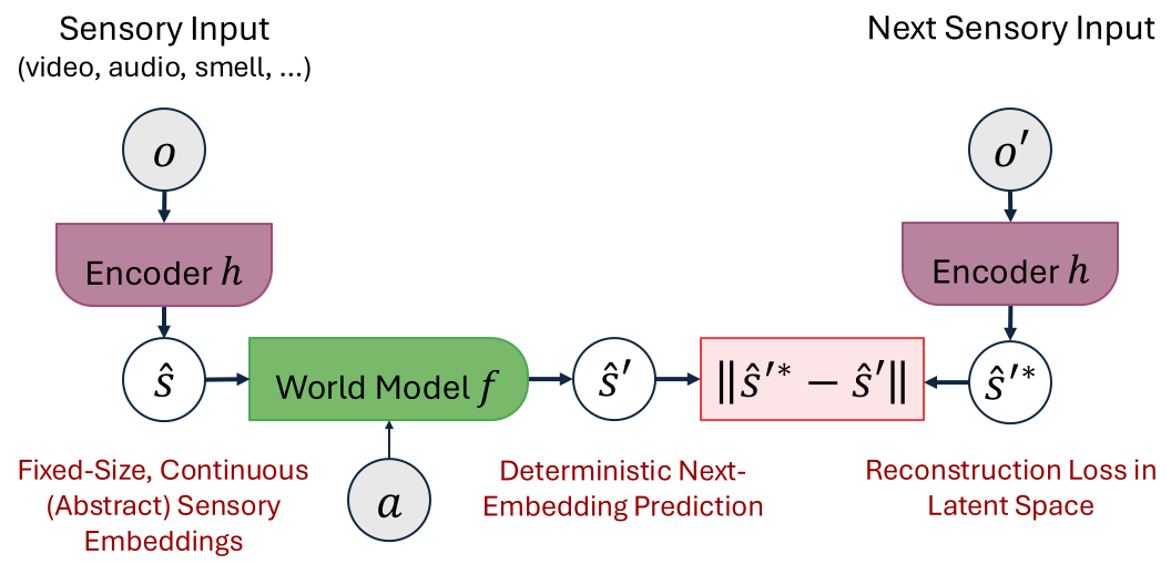
The critique examines five design preferences: sensory-first data, continuous embeddings, decoder-free latent prediction, latent-space losses, and online model-predictive control. It argues for alternatives or combinations according to the desired scope of the system.
Figure 3: A systematic technical proposal that results from common wisdom on world modeling, most prominently instantiated by the joint embedding predictive architecture (JEPA).
4.1 Data: Information Density, Not Just Volume
Raw byte count does not measure useful information. Language compactly records concepts, explanations, and social knowledge; sensory streams provide physical detail and grounding. The authors favor learning from their complementary roles instead of selecting one modality by volume alone.
4.2 Representation: Continuous? Discrete? Or Both?
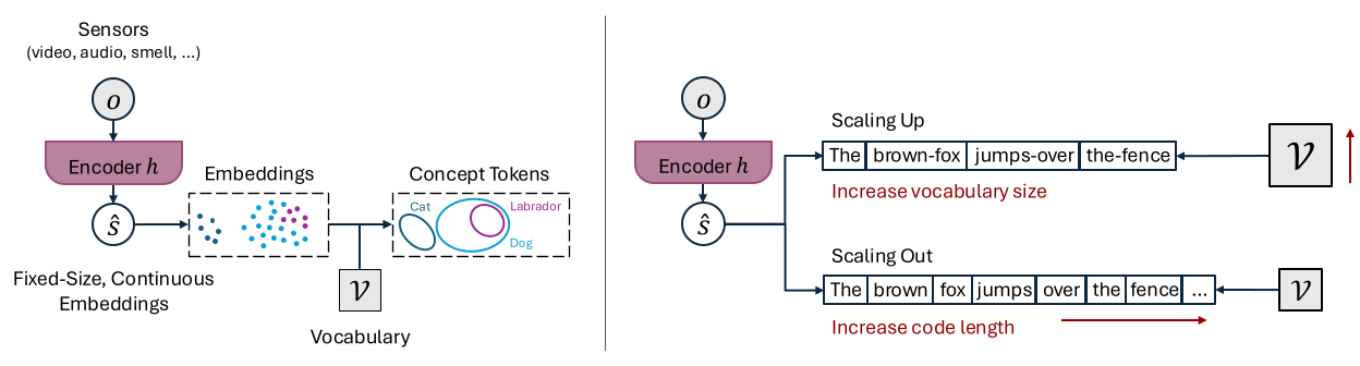
The proposed representation combines discrete concepts for compositional reasoning with continuous features for fine perceptual variation. “Stateful” here means a persistent, identifiable estimate useful for predicting relevant dynamics. Discreteness alone does not establish that property, and a compressed continuous representation can also preserve sufficient task information.
Theorem 1 gives a bounded-input, finite-resolution encoding argument: sufficiently different real-valued inputs can receive distinct finite token sequences. Increasing sequence length avoids the rapidly growing vocabulary in the particular fixed-length construction. This establishes representational capacity, not semantic understanding, exact lossless encoding, learnability, or a general compute-efficiency advantage. [55]
Figure 4: Vocabulary-based tokens is an effective way to categorize perceptual inputs into discrete concepts for reasoning (left). We may scale up or scale out discrete code to deal with increasing data complexity (right). Thm.1 shows either is effective, but scaling out is more efficient.
4.3 Architecture: Pure Abstraction, or Autoregressive Generation
The architectural proposal combines latent reasoning with a decoder that lets predictions be checked against observations.
4.3.1 Two Competing Approaches
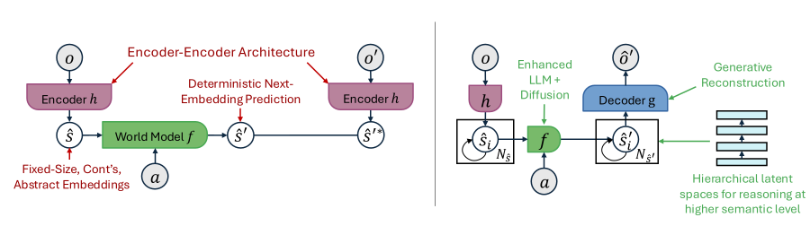
Observation-generating systems explicitly reconstruct outputs; JEPA-style systems predict a target embedding. Repeated latent prediction still rolls a state forward recursively, even without a probabilistic observation decoder. The authors distinguish this functional simulation from sampling uncertain outcomes.
Equations
Figure 5: Comparison of the joint embedding predictive architecture (JEPA, left) and the proposed Generative Latent Prediction (GLP) architecture (right). JEPA operates in open loop, predicting the next latent state without reconstructing observations. GLP closes the loop through a decoder that validates predictions against observable data, while incorporating both an enhanced LLM backbone for discrete reasoning and a diffusion-based predictor for continuous dynamics.
4.3.2 Tradeoffs for General-Purpose Modeling
Abstraction can discard information needed by an unforeseen task, while reconstruction can spend capacity on irrelevant detail. The authors prefer reconstruction as a diagnostic and training signal for broadly useful representations. The argument is a design trade-off: lossy encoders can retain sufficient dynamics, and reconstruction alone does not guarantee that every important fact or rare event is modeled.
4.3.3 Generative Latent Prediction as a Synthesis
GLP places continuous generative prediction at a perceptual level, learned discrete tokens at an intermediate level, and language-based reasoning above them. An enhanced LLM and diffusion predictor exchange information within an encoder–decoder system. Claimed improvements in long-horizon reasoning and stability are architectural motivations requiring empirical evaluation.
4.4 Objective: Learning in Data Space, or Latent Space?
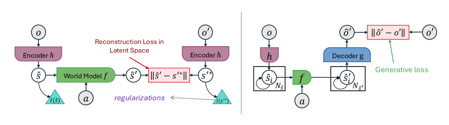
The unregularized latent loss admits a constant encoder and constant predictor with zero error: Proposition 1 establishes this collapsed optimum. It does not show that practical JEPA methods with additional training mechanisms necessarily collapse.
Proposition 2 claims reconstruction excludes such optima, but its proof requires decoder access to the target observations and independently distinguishable inputs. Distinct stochastic outcomes for the same input can still have an optimal constant deterministic prediction.
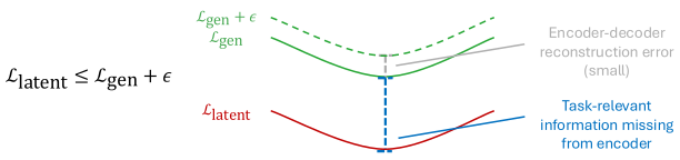
Reading note: Theorem 2 claims latent error is at most observation error plus round-trip error. This does not follow from its stated assumptions. For scalar h(o)=2o, g(s)=s/2, f=0, and next observation 1, round-trip error is zero, yet latent error is 2 and observation error is 1. The original formulas and diagram remain below; they should not be treated as an established universal ordering of the two objectives.
Equations 7–8
(7)
(8)
Figure 6: Comparison of latent-space reconstruction objectives (left) and generative data reconstruction objectives (right).Equations
Figure 7: As Thm. 2 shows, the energy-based latent reconstruction loss () is upper bounded by the generative data reconstruction loss () plus a small encoder-decoder reconstruction error (). is small in practice, meaning usually holds. Minimizing , therefore, does not guarantee consistency with observed data, which is required for minimizing .
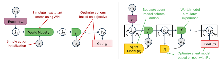
MPC repeatedly simulates candidate action sequences at decision time. Learning a policy from model-generated rollouts shifts some computation into training and can make later action selection faster. Both approaches still depend on model accuracy and can be combined with planning, value functions, or reactive control.
The authors favor using world models for learning as well as inference. Their discussion does not establish that MPC is generally limited to short-sighted behavior or that model-based RL automatically avoids unsafe or inaccurate imagined experience.
Equation
Figure 8: Comparison of model-predictive control (left) and reinforcement learning from world-model-simulated experience (right) as approaches to using the world model for decision-making.Equation 9
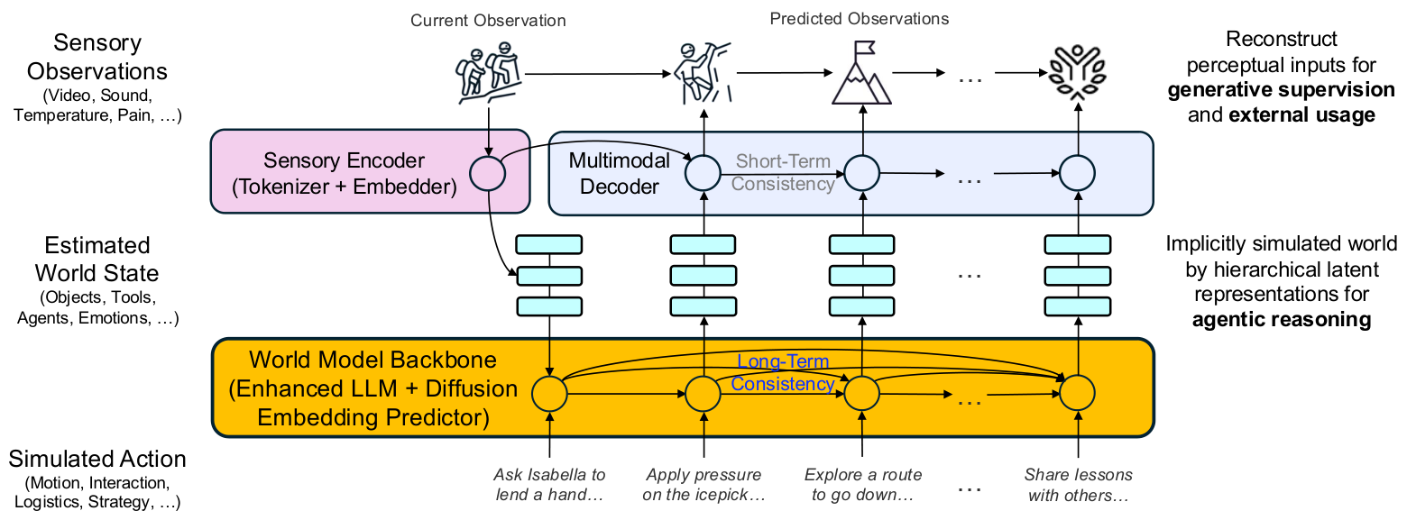
PAN instantiates the proposed principles: multimodal experience, persistent mixed representations, hierarchical GLP prediction, observation-based supervision, and simulated experience for agents. Figure 9 summarizes the intended information flow.
Figure 9: Illustration of the generative latent prediction (GLP) architecture of PAN-World, our proposed framework for general-purpose world modeling. At each time point, PAN-World estimates the world state based on the current sensory observation , predicts the future world states based on proposed actions for agentic reasoning, and reconstructs the future observations for generative supervision and external usage.
5.1 A Motivating Usecase
A mountaineering expedition illustrates the desired range: route planning, gear use, movement, weather assessment, and social coordination operate at different time and spatial scales. This is a motivating scenario, not a reported deployment or task-success experiment.
A sensory encoder produces learned discrete tokens and continuous embeddings. An LLM handles conceptual sequences, a diffusion predictor handles detailed perceptual transitions, and a learned switch chooses how to combine them. A multimodal decoder reconstructs predicted observations.
The factorization describes hierarchical state inference and next-state prediction. Dynamic vocabulary growth and persistent memory are proposed mechanisms; this essay does not measure their reliability or establish general-purpose state sufficiency.
Modules are first pretrained on suitable modality-specific data, then aligned through multimodal post-training. The proposal uses text for broad conceptual knowledge and physical observations for embodied detail, aiming to combine knowledge without requiring complete demonstrations of every complex task. Its sample-efficiency advantages are expectations rather than quantified results here.
A PAN agent would precompute and cache candidate futures, then consult them alongside current beliefs and goals. This separates some simulation effort from immediate action selection. The section outlines an agent design rather than a validated solution to open-ended planning.
Figure 10: Illustration of our proposed simulative reasoning agent powered by the PAN World Model. Unlike traditional RL agents that rely on reactive policies, or model-precitive control (MPC) agents that expensively simulates futures at decision time, this agent leverages a cache of precomputed simulations generated by the PANWM. During decision-making, the agent selects actions based on its current beliefs and expected outcomes, enabling a more efficient, flexible, and intentional form of planning, which, as we argue, is closer to the flexibility of human reasoning.
6 Conclusion
The essay’s main contribution is a synthesis of world-model design choices and a proposal for mixed, hierarchical, observation-grounded simulation. Wider generalization, multiple agents, long time scales, and learning from imagined experience remain research directions. Evaluating those ambitions requires evidence beyond the architectural sketch and the qualified theoretical arguments.
Appendix A Proof for Theorem 1
The proof quantizes each coordinate of a bounded input finely enough that equal codes imply a bounded reconstruction difference. It constructs either a large vocabulary with fixed-length codes or longer base-coded sequences with a fixed vocabulary.
This is a finite-precision existence argument. The printed proof has inconsistent norm, index, and vocabulary-size notation; its central quantization idea does not establish natural-language semantics or compare total storage bits and runtime.
Equations 10–12
(10)
(11)
(12)
Appendix B Proof for Proposition 1
Choose any constant latent vector. Map every observation to it and every encoded state–action pair back to it. The latent reconstruction loss is then zero, a global minimum of this nonnegative unregularized objective.
Appendix C Proof for Proposition 2
The proposed proof changes the representation and prediction for two examples so that a fixed decoder reproduces their distinct targets, leaving other outputs unchanged. That construction assumes suitable decoder preimages and independently adjustable inputs.
Those conditions are stronger than merely having two distinct next observations. A constant fixed decoder cannot improve at all, and incompatible targets for the same input cannot both be fitted by the deterministic predictor. Reconstruction can discourage collapse without the unconditional guarantee stated in the proposition.
Equations
Appendix D Proof of Theorem 2
The proof tries to compare Gaussian KL divergences using data processing, then apply round-trip consistency and the triangle inequality. Its key step treats an encoded observation Gaussian as a unit-covariance latent Gaussian. A general encoder does not preserve that covariance or even Gaussianity.
Consequently, the claimed bound and equality under exact inversion do not follow. The scalar scaling counterexample in Section 4.4 already violates both despite a perfect encoder–decoder round trip. Additional metric or distributional assumptions would be needed.
Equations 13–14
(13)
(14)
72 references
[1]N. Agarwal, A. Ali, M. Bala, Y. Balaji, E. Barker, T. Cai, P. Chattopadhyay, Y. Chen, Y. Cui, Y. Ding, et al. (2025)Cosmos world foundation model platform for physical ai.
arXiv preprint arXiv:2501.03575.
[3]A. Ali, J. Bai, M. Bala, Y. Balaji, A. Blakeman, T. Cai, J. Cao, T. Cao, E. Cha, Y. Chao, et al. (2025)World simulation with video foundation models for physical ai.
arXiv preprint arXiv:2511.00062.
[4]M. Assran, A. Bardes, D. Fan, Q. Garrido, R. Howes, Mojtaba, Komeili, M. Muckley, A. Rizvi, C. Roberts, K. Sinha, A. Zholus, S. Arnaud, A. Gejji, A. Martin, F. R. Hogan, D. Dugas, P. Bojanowski, V. Khalidov, P. Labatut, F. Massa, M. Szafraniec, K. Krishnakumar, Y. Li, X. Ma, S. Chandar, F. Meier, Y. LeCun, M. Rabbat, and N. Ballas (2025)V-jepa 2: self-supervised video models enable understanding, prediction and planning.
External Links: 2506.09985,
Link
[5]L. J. Ball (2020)Hypothetical thinking.
In The Cambridge Handbook of the Imagination, A. Abraham (Ed.),
Cambridge Handbooks in Psychology, pp. 514–528.
[6]P. J. Ball, J. Bauer, F. Belletti, B. Brownfield, A. Ephrat, S. Fruchter, A. Gupta, K. Holsheimer, A. Holynski, J. Hron, C. Kaplanis, M. Limont, M. McGill, Y. Oliveira, J. Parker-Holder, F. Perbet, G. Scully, J. Shar, S. Spencer, O. Tov, R. Villegas, E. Wang, J. Yung, C. Baetu, J. Berbel, D. Bridson, J. Bruce, G. Buttimore, S. Chakera, B. Chandra, P. Collins, A. Cullum, B. Damoc, V. Dasagi, M. Gazeau, C. Gbadamosi, W. Han, E. Hirst, A. Kachra, L. Kerley, K. Kjems, E. Knoepfel, V. Koriakin, J. Lo, C. Lu, Z. Mehring, A. Moufarek, H. Nandwani, V. Oliveira, F. Pardo, J. Park, A. Pierson, B. Poole, H. Ran, T. Salimans, M. Sanchez, I. Saprykin, A. Shen, S. Sidhwani, D. Smith, J. Stanton, H. Tomlinson, D. Vijaykumar, L. Wang, P. Wingfield, N. Wong, K. Xu, C. Yew, N. Young, V. Zubov, D. Eck, D. Erhan, K. Kavukcuoglu, D. Hassabis, Z. Gharamani, R. Hadsell, A. van den Oord, I. Mosseri, A. Bolton, S. Singh, and T. Rocktäschel (2025)Genie 3: a new frontier for world models.
External Links:
[7]A. Bardes, Q. Garrido, J. Ponce, X. Chen, M. Rabbat, Y. LeCun, M. Assran, and N. Ballas (2024)Revisiting feature prediction for learning visual representations from video.
arXiv preprint arXiv:2404.08471.
[9]L. E. Baum and T. Petrie (1966)Statistical inference for probabilistic functions of finite state markov chains.
The Annals of Mathematical Statistics37 (6), pp. 1554–1563.
External Links: Document
[10]T. Brooks, B. Peebles, C. Holmes, W. DePue, Y. Guo, L. Jing, D. Schnurr, J. Taylor, T. Luhman, E. Luhman, et al. (2024)Video generation models as world simulators. 2024.
URL https://openai. com/research/video-generation-models-as-world-simulators3, pp. 1.
[12]M. Caron, H. Touvron, I. Misra, H. Jégou, J. Mairal, P. Bojanowski, and A. Joulin (2021)Emerging properties in self-supervised vision transformers.
In Proceedings of the IEEE/CVF international conference on computer vision,
pp. 9650–9660.
[13]Y. Chervonyi, T. H. Trinh, M. Olšák, X. Yang, H. Nguyen, M. Menegali, J. Jung, V. Verma, Q. V. Le, and T. Luong (2025)Gold-medalist performance in solving olympiad geometry with alphageometry2.
arXiv preprint arXiv:2502.03544.
[14]B. Chiou, M. Choey, M. Deng, J. Hou, J. Wang, A. Wu, F. Xu, Z. Hu, H. Jin, L. E. Li, G. Neubig, Y. Shen, and E. P. Xing (2025)ReasonerAgent: a fully open source, ready-to-run agent that does research in a web browser and answers your queries.
External Links: Link
[17]M. Deng, J. Hou, Z. Hu, G. Neubig, H. Jin, Y. Shen, and E. P. Xing (2025)SimuRA: towards general goal-oriented agent via simulative reasoning architecture with llm-based world model.
External Links: Link
[21]D. Guo, D. Yang, H. Zhang, J. Song, R. Zhang, R. Xu, Q. Zhu, S. Ma, P. Wang, X. Bi, et al. (2025)Deepseek-r1: incentivizing reasoning capability in llms via reinforcement learning.
arXiv preprint arXiv:2501.12948.
[23]S. Hao, Y. Gu, H. Ma, J. J. Hong, Z. Wang, D. Z. Wang, and Z. Hu (2023)Reasoning with language model is planning with world model.
arXiv preprint arXiv:2305.14992.
[24]K. He, X. Chen, S. Xie, Y. Li, P. Dollár, and R. Girshick (2022)Masked autoencoders are scalable vision learners.
In Proceedings of the IEEE/CVF conference on computer vision and pattern recognition,
pp. 16000–16009.
[29]A. Kanervisto, D. Bignell, L. Y. Wen, M. Grayson, R. Georgescu, S. Valcarcel Macua, S. Z. Tan, T. Rashid, T. Pearce, Y. Cao, et al. (2025)World and human action models towards gameplay ideation.
Nature638 (8051), pp. 656–663.
[31]Y. LeCun and E. Xing (2026)How should ai learn to understand the world? yann lecun & eric xing on jepa and glp(Website)
Spring School AI for Impact.
Note: YouTube video; debate at Spring School AI for Impact 2026, Ben Guerir, Morocco, March 25, 2026External Links: Link
[35]W. E. McNelly (Ed.) (1984)The dune encyclopedia.
Berkley Publishing Group, New York.
Note: Published by arrangement with the author. Designed by Jeremiah B. LighterExternal Links: ISBN 0-425-06813-7
[36]C. Mitra, B. Huang, T. Darrell, and R. Herzig (2024)Compositional chain-of-thought prompting for large multimodal models.
In Proceedings of the IEEE/CVF Conference on Computer Vision and Pattern Recognition,
pp. 14420–14431.
[39]J. Parker-Holder, P. Ball, J. Bruce, V. Dasagi, K. Holsheimer, C. Kaplanis, A. Moufarek, G. Scully, J. Shar, J. Shi, S. Spencer, J. Yung, M. Dennis, S. Kenjeyev, S. Long, V. Mnih, H. Chan, M. Gazeau, B. Li, F. Pardo, L. Wang, L. Zhang, F. Besse, T. Harley, A. Mitenkova, J. Wang, J. Clune, D. Hassabis, R. Hadsell, A. Bolton, S. Singh, and T. Rocktäschel (2024)Genie 2: a large-scale foundation world model.
External Links: Link
[42]A. Radford, J. W. Kim, C. Hallacy, A. Ramesh, G. Goh, S. Agarwal, G. Sastry, A. Askell, P. Mishkin, J. Clark, et al. (2021)Learning transferable visual models from natural language supervision.
In International conference on machine learning,
pp. 8748–8763.
[43]R. Rombach, A. Blattmann, D. Lorenz, P. Esser, and B. Ommer (2022)High-resolution image synthesis with latent diffusion models.
In Proceedings of the IEEE/CVF conference on computer vision and pattern recognition,
pp. 10684–10695.
[44]R. Y. Rubinstein (1997)Optimization of computer simulation models with rare events.
European Journal of Operational Research99 (1), pp. 89–112.
External Links: ISSN 0377-2217,
Document,
Link
[46]L. Russell, A. Hu, L. Bertoni, G. Fedoseev, J. Shotton, E. Arani, and G. Corrado (2025)Gaia-2: a controllable multi-view generative world model for autonomous driving.
arXiv preprint arXiv:2503.20523.
[47]D. Silver, A. Huang, C. J. Maddison, A. Guez, L. Sifre, G. Van Den Driessche, J. Schrittwieser, I. Antonoglou, V. Panneershelvam, M. Lanctot, et al. (2016)Mastering the game of go with deep neural networks and tree search.
nature529 (7587), pp. 484–489.
[48]D. Silver, T. Hubert, J. Schrittwieser, I. Antonoglou, M. Lai, A. Guez, M. Lanctot, L. Sifre, D. Kumaran, T. Graepel, et al. (2017)Mastering chess and shogi by self-play with a general reinforcement learning algorithm.
arXiv preprint arXiv:1712.01815.
[49]O. Siméoni, H. V. Vo, M. Seitzer, F. Baldassarre, M. Oquab, C. Jose, V. Khalidov, M. Szafraniec, S. Yi, M. Ramamonjisoa, et al. (2025)Dinov3.
arXiv preprint arXiv:2508.10104.
[50]V. Sobal, W. Zhang, K. Cho, R. Balestriero, T. G. Rudner, and Y. LeCun (2025)Learning from reward-free offline data: a case for planning with latent dynamics models.
arXiv preprint arXiv:2502.14819.
[52]Q. Sun, X. Huang, J. Gu, B. C. Williams, and H. Zhao (2022)M2i: from factored marginal trajectory prediction to interactive prediction.
In Proceedings of the IEEE/CVF Conference on Computer Vision and Pattern Recognition,
pp. 6543–6552.
[54]R. Team, Z. Gao, Q. Wang, Y. Zeng, J. Zhu, K. L. Cheng, Y. Li, H. Wang, Y. Xu, S. Ma, et al. (2026)Advancing open-source world models.
arXiv preprint arXiv:2601.20540.
[56]N. Van Hoeck, P. D. Watson, and A. K. Barbey (2015)Cognitive neuroscience of human counterfactual reasoning.
Frontiers in human neuroscience9, pp. 420.
[57]B. Varadarajan, A. Hefny, A. Srivastava, K. S. Refaat, N. Nayakanti, A. Cornman, K. Chen, B. Douillard, C. P. Lam, D. Anguelov, et al. (2022)Multipath++: efficient information fusion and trajectory aggregation for behavior prediction.
In 2022 International Conference on Robotics and Automation (ICRA),
pp. 7814–7821.
[59]D. Wang, H. Jung, T. Monnier, K. Sohn, C. Zou, X. Xiang, Y. Yeh, D. Liu, Z. Huang, T. Nguyen-Phuoc, et al. (2025)WorldGen: from text to traversable and interactive 3d worlds.
arXiv preprint arXiv:2511.16825.
[60]X. Wang, B. Li, Y. Song, F. F. Xu, X. Tang, M. Zhuge, J. Pan, Y. Song, B. Li, J. Singh, et al. (2024)Openhands: an open platform for ai software developers as generalist agents.
In The Thirteenth International Conference on Learning Representations,
[63]G. Williams, A. Aldrich, and E. Theodorou (2015)Model predictive path integral control using covariance variable importance sampling.
arXiv preprint arXiv:1509.01149.
[66]J. Xiang, Y. Gu, Z. Liu, Z. Feng, Q. Gao, Y. Hu, B. Huang, G. Liu, Y. Yang, K. Zhou, et al. (2025)Pan: a world model for general, interactable, and long-horizon world simulation.
arXiv preprint arXiv:2511.09057.
[67]J. Xiang, G. Liu, Y. Gu, Q. Gao, Y. Ning, Y. Zha, Z. Feng, T. Tao, S. Hao, Y. Shi, et al. (2024)Pandora: towards general world model with natural language actions and video states.
arXiv preprint arXiv:2406.09455.
[68]J. Xiang, T. Tao, Y. Gu, T. Shu, Z. Wang, Z. Yang, and Z. Hu (2023)Language models meet world models: embodied experiences enhance language models.
Advances in neural information processing systems36, pp. 75392–75412.
[70]P. Zhang, Y. Chen, H. Huang, W. Lin, Z. Liu, I. Stoica, E. Xing, and H. Zhang (2026)Faster video diffusion with trainable sparse attention.
Advances in Neural Information Processing Systems38, pp. 152509–152534.
[71]P. Zhang, Y. Chen, R. Su, H. Ding, I. Stoica, Z. Liu, and H. Zhang (2025)Fast video generation with sliding tile attention.
arXiv preprint arXiv:2502.04507.
[72]G. Zhou, H. Pan, Y. LeCun, and L. Pinto (2024)Dino-wm: world models on pre-trained visual features enable zero-shot planning.
arXiv preprint arXiv:2411.04983.