A compositional method learns stable linear parameter-varying dynamical systems (LPV-DS) from high-dimensional demonstrations. It fits smaller interconnected subsystems, then searches for a global stability certificate. Seven-dimensional robot-joint examples become tractable where the tested monolithic optimization fails, and a physical arm tracks the learned motions.
I Introduction
Joint-space learning can preserve demonstrated coordination and orientation without inverse kinematics, but stable LPV-DS fitting becomes numerically difficult as dimension grows. The proposed divide-and-conquer method retains the joint coordinates, partitions the dynamics into coupled subsystems, and certifies their interconnection. It targets the bilinear matrix inequalities (BMIs) that make direct fitting nonconvex.
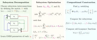
Fig. 1: Our proposed approach consists of three main steps: subsystem decomposition, subsystem-level optimization and compositional construction of the DS and of the Lyapunov function certifying its stability.
II Preliminaries
States are concatenations of subsystem coordinates. Symmetric matrix inequalities express positivity, while the interconnection matrix specifies which coordinates serve as inputs to each subsystem.
II-A Learning Stable Dynamical Systems
Demonstrated position–velocity pairs define a regression objective with a chosen equilibrium and Lyapunov decrease constraints. An LPV model combines local linear dynamics through Gaussian mixture model (GMM) weights. Searching jointly for dynamics and a general quadratic Lyapunov function gives expressive models but introduces nonconvex bilinear constraints.
Equations 1–5
(1)
(2a)
such that
(2b)
(2c)
(2d)
(3)
(4)
(5)
II-B Interconnected Systems
Each subsystem has its own state and internal inputs. A fixed interconnection matrix couples these inputs to the other subsystem states. The resulting vector field is assembled from all local vector fields; subsystem fitting alone does not establish stability of the interconnected model.
Equations 6–8
(6)
(7)
(8)
III Compositional Framework
Each local optimization fits demonstration velocities together with a sub-Lyapunov function and a matrix describing its interaction with other subsystems. Theorem 1 gives sufficient global coupling conditions so a weighted sum of these functions certifies the full system. Theorem 2 expresses local conditions as linear and bilinear matrix inequalities for LPV subsystems. The retained algorithm fits GMMs, solves the local problems, and then finds the global certificate. The decomposition is chosen manually and can affect accuracy and computation; automated selection remains future work.
Equations 9a–23
(9a)
such that
(9b)
(9c)
(20)
(21)
(22)
(23)
Algorithm 1Proposed Framework
Input:Demonstrated data
Output:Dynamics and Lyapunov function
Initialize: Shift equilibrium point to origin;
Subsystem Decomposition
Choose subsystem configuration and specify connections defining the matrix :
Replace the numerical values of the found matrices and in the quadratic inequality (3) and find that satisfy this constraint ;
Let
;
;
Define the interconnected system dynamics and Lyapunov function as:;
, ;
IV Simulation
Two seven-dimensional joint-space datasets are fitted in MATLAB R2024a using YALMIP and PENLAB on an Apple M2 MacBook Pro with 8 GB of memory. Results concern these datasets and solver configurations, rather than a universal complexity or convergence bound.
IV-A Example 1: Individual Joint Subsystems
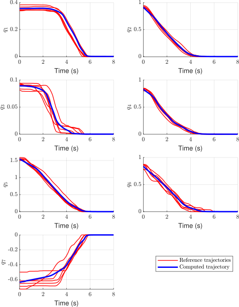
Using one subsystem per joint, local optimization takes about 92 seconds and composition another 9 seconds. Table I reports mean squared error 2.76 in 101 seconds, versus 3.39 in 72.35 seconds for the stable neural dynamical system baseline (SNDS). The monolithic LPV-DS solver does not converge in this example. The compositional method is therefore more accurate here, but not faster than SNDS.
Fig. 2: Comparison between demonstrated trajectories (red) in the joint-space and a generated trajectory (blue) from the learned DS using our proposed algorithm with the interconnection defined in Example 1.
IV-B Example 2: Flexible Subsystem Structure
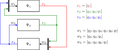
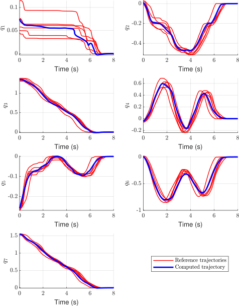
A second hand-selected coupling structure models a more curved trajectory. Table I reports error 0.37 in 146.32 seconds, versus SNDS error 7.00 in 559.66 seconds after 1,000 epochs; the 150-epoch neural run and monolithic LPV-DS fit fail. The prose gives a slightly different 146.36-second runtime, so the table value is used here.
TABLE I: Comparison of mean squared error (MSE) and run time in seconds. The symbol indicates the learning method failed to produce a stable DS due to numerical error or solver failure.
Fig. 3: Interconnection between subsystems in Example 2.Fig. 4: Comparison between demonstrated trajectories (red) in the joint-space and a generated trajectory (blue) from the learned DS using our proposed algorithm with the interconnection defined in Example 2.
V Experiment
A seven-degree-of-freedom Franka Emika arm tracks the learned joint velocities through its internal joint impedance controller. The Franka Control Interface (FCI) runs at 1 kHz on an Intel i5 workstation with a real-time Linux kernel.
V-A Experiment 1
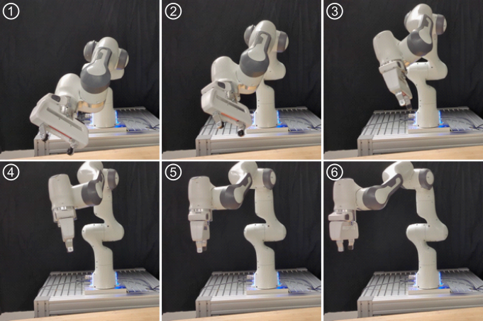
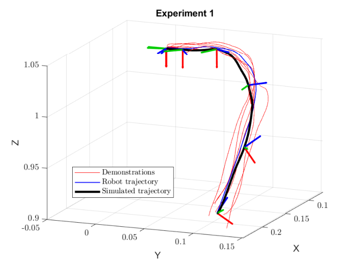
The first physical experiment reproduces a nonlinear motion with varying end-effector position and orientation. Recorded trajectories closely follow the demonstrations, illustrating the benefit of learning coordinated joint motion directly.
Fig. 5: Experimental setup corresponding to Experiment 1. The task is to move the end effector sequentially through poses \raisebox{-0.9pt}{1}⃝ to \raisebox{-0.9pt}{6}⃝, matching the pose shown in the corresponding snapshots.
Fig. 6: Reference trajectories (red), DS-generated trajectory (blue), and trajectory executed by the DS-controlled robot (black) are shown in the task space, along with orientations using RGB stick axes.
V-B Experiment 2
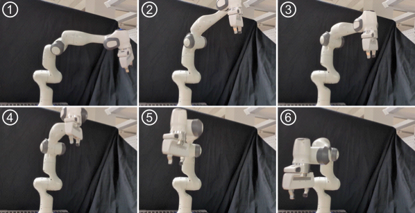
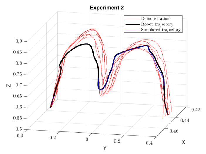
The second dataset demonstrates extracting an object from a box along a curved path. The learned model reproduces the motion while avoiding the walls in the shown experiment. Stability toward an equilibrium does not itself certify obstacle avoidance everywhere; the paper does not establish a general collision-safety guarantee for this learned field.
Fig. 7: Experimental setup corresponding to Experiment 2. The task is to move the end effector sequentially through poses \raisebox{-0.8pt}{1}⃝
to \raisebox{-0.8pt}{6}⃝, matching the pose shown in the corresponding snapshots.
Fig. 8: Reference trajectories (red), DS-generated trajectory (blue), and trajectory executed by the DS-controlled robot (black) are shown in the task space.
VI Conclusion
Decomposing the nonconvex fit makes these high-dimensional LPV models practical to learn in minutes. The method still relies on successful numerical local solves and a feasible interconnection certificate. The experiments demonstrate seven-dimensional scalability and reproduction of two motions; broader scaling and automatic decomposition are open.
Appendix A
The appendix proves the composition and LPV matrix-inequality results under their stated assumptions.
Proof of Theorem 1
The demonstration-fitting objective separates by subsystem coordinates. Bounds on local sub-Lyapunov functions and the coupling inequality then establish a positive global Lyapunov function and a negative derivative for the interconnected dynamics.
Equations
Proof of Theorem 2
Substituting quadratic sub-Lyapunov functions converts the required bounds into matrix inequalities. Each local linear component satisfies the derivative condition, and nonnegative GMM weights preserve it when the components are mixed.
Equations 24–25
(24)
(25)
25 references
[1]
A. Billard, S. Calinon, R. Dillmann, and S. Schaal, Robot Programming by Demonstration. Berlin, Heidelberg: Springer Berlin Heidelberg, 2008, pp. 1371–1394.
[2]
B. Argall, S. Chernova, M. Veloso, and B. Browning, “A survey of robot learning from demonstration,” Robotics and Autonomous Systems, vol. 57, pp. 469–483, 05 2009.
[3]
H. Ravichandar, A. S. Polydoros, S. Chernova, and A. Billard, “Recent advances in robot learning from demonstration,” Annual review of control, robotics, and autonomous systems, vol. 3, no. 1, pp. 297–330, 2020.
[5]
Y. Shavit, N. Figueroa, S. S. M. Salehian, and A. Billard, “Learning augmented joint-space task-oriented dynamical systems: a linear parameter varying and synergetic control approach,” IEEE Robotics and Automation Letters, vol. 3, no. 3, pp. 2718–2725, 2018.
[6]
A. Ude, B. Nemec, T. Petrić, and J. Morimoto, “Orientation in Cartesian space dynamic movement primitives,” in 2014 IEEE International Conference on Robotics and Automation (ICRA). IEEE, 2014, pp. 2997–3004.
[8]
M. J. A. Zeestraten, I. Havoutis, J. a. Silvério, S. Calinon, and D. G. Caldwell, “An approach for imitation learning on Riemannian manifolds,” IEEE Robotics and Automation Letters, vol. 2, no. 3, pp. 1240–1247, 2017.
[9]
N. Figueroa and A. Billard, “A physically-consistent Bayesian non-parametric mixture model for dynamical system learning,” in Conference on Robot Learning. PMLR, 2018, pp. 927–946.
[10]
——, “Locally active globally stable dynamical systems: theory, learning, and experiments,” The International Journal of Robotics Research, vol. 41, no. 3, pp. 312–347, 2022.
[11]
O. Toker and H. Ozbay, “On the NP-hardness of solving bilinear matrix inequalities and simultaneous stabilization with static output feedback,” in Proceedings of 1995 American Control Conference, vol. 4. IEEE, 1995, pp. 2525–2526.
[12]
M. Fukuda and M. Kojima, “Branch-and-cut algorithms for the bilinear matrix inequality eigenvalue problem,” Computational Optimization and Applications, vol. 19, pp. 79–105, 2001.
[13]
P. Roux, Y.-L. Voronin, and S. Sankaranarayanan, “Validating numerical semidefinite programming solvers for polynomial invariants,” Formal Methods in System Design, vol. 53, pp. 286–312, 2018.
[14]
A. Abyaneh and H.-C. Lin, “Learning Lyapunov-stable polynomial dynamical systems through imitation,” in Proceedings of the 2023 Conference on Robot Learning (CoRL 2023), 2023.
[15]
M. Schonger, H. T. Kussaba, L. Chen, L. Figueredo, A. Swikir, A. Billard, and S. Haddadin, “Learning barrier-certified polynomial dynamical systems for obstacle avoidance with robots,” in Proceedings of the 2024 International Conference on Robotics and Automation, 2024, pp. 17 201–17 207.
[16]
S. M. Khansari-Zadeh and A. Billard, “Learning stable nonlinear dynamical systems with Gaussian mixture models,” IEEE Transactions on Robotics, vol. 27, no. 5, pp. 943–957, Oct. 2011.
[18]
M. A. Rana, A. Li, D. Fox, B. Boots, F. Ramos, and N. Ratliff, “Euclideanizing flows: Diffeomorphic reduction for learning stable dynamical systems,” in Learning for Dynamics and Control. PMLR, 2020, pp. 630–639.
[19]
N. Lawrence, P. Loewen, M. Forbes, J. Backstrom, and B. Gopaluni, “Almost surely stable deep dynamics,” Advances in Neural Information Processing Systems, vol. 33, pp. 18 942–18 953, 2020.
[20]
A. Abyaneh, M. S. Guzmán, and H.-C. Lin, “Globally stable neural imitation policies,” in 2024 IEEE International Conference on Robotics and Automation (ICRA). IEEE, 2024, pp. 15 061–15 067.
[21]
M. Arcak, C. Meissen, and A. Packard, Networks of dissipative systems: compositional certification of stability, performance, and safety. Springer, 2016.
[24]
J. Löfberg, “YALMIP: A toolbox for modeling and optimization in MATLAB,” in 2004 IEEE international conference on robotics and automation. IEEE, 2004, pp. 284–289.
[25]
S. Haddadin, S. Parusel, L. Johannsmeier, S. Golz, S. Gabl, F. Walch, M. Sabaghian, C. Jaehne, L. Hausperger, and S. Haddadin, “The Franka Emika robot: A reference platform for robotics research and education,” IEEE Robotics & Automation Magazine, 2022.