Overview
The supplement expands the generative-model background, spatial-consistency metric, camera-rotation and object-editing galleries, and limitations. All 16 numbered figures, five numbered tables with seven data panels, eight appendix equations and the main-text mathematical definitions are retained.
At a glance
BEV-VAE compresses synchronized surround-camera images into one spatially organized bird’s-eye-view latent representation. A camera-conditioned decoder reconstructs views, while a separately trained diffusion transformer generates new latent scenes from noise and optional 3D box occupancy. The experiments show useful reconstruction, modest camera-rotation synthesis and object-layout edits on nuScenes and Argoverse 2. Shared coordinates provide a geometric inductive bias; they do not guarantee physically correct images or consistent object identity.
1 Introduction
Generating each camera image independently makes overlapping views difficult to align, while projecting 3D boxes into 2D can discard depth relationships. This work instead assigns the scene a common BEV latent grid and conditions generation on 3D occupancy. Camera extrinsics choose which view the decoder produces, without retraining for each demonstrated rotation.
The evidence concerns static multi-view image generation at 256×256 resolution. Claims about synthetic data helping autonomous driving motivate the work; no downstream driving, planning or safety improvement is measured. “Arbitrary view” is broader than the demonstrated rotations, which range up to ±15° around the original cameras.

2 Related Work
The design combines BEV perception, a variational image bottleneck and latent diffusion. Its distinction is where generation occurs and how geometric conditioning enters, rather than inventing these components.
2.1 Bird’s-Eye-View Perception
Bottom-up BEV methods lift image features using estimated depth. Top-down approaches query spatial reference points and gather projected image features with deformable attention [8][9]. Each attention head learns sampling offsets and weights, with bilinear interpolation of sampled features. The original attention formula and weight normalization are retained below; q is a query, p a reference location, v the value features, M the heads and K the sampled keys.
Equations
2.2 Variational Autoencoder
The VAE learns a Gaussian posterior and reconstruction decoder. Prior vector-quantized and adversarial variants improve perceptual quality, while latent diffusion moves iterative denoising into a compressed representation [10][11][18]. Here the latent representation covers a multi-camera scene, and a DiT transformer models its distribution [19]. The method uses pretrained perceptual features even though its generative backbone is trained without a Stable Diffusion prior.
2.3 Autonomous Driving Multi-view Generation
BEVGen uses autoregressive generation from BEV layouts [20]. MagicDrive, DrivingDiffusion and Panacea use diffusion with different camera/layout encodings and cross-view interactions [1][2][4], while DriveWM models multi-view relations in a world-model setting [3]. Comparisons therefore differ in pretraining, conditions and architecture; they do not isolate the effect of BEV representation alone.
3 Method
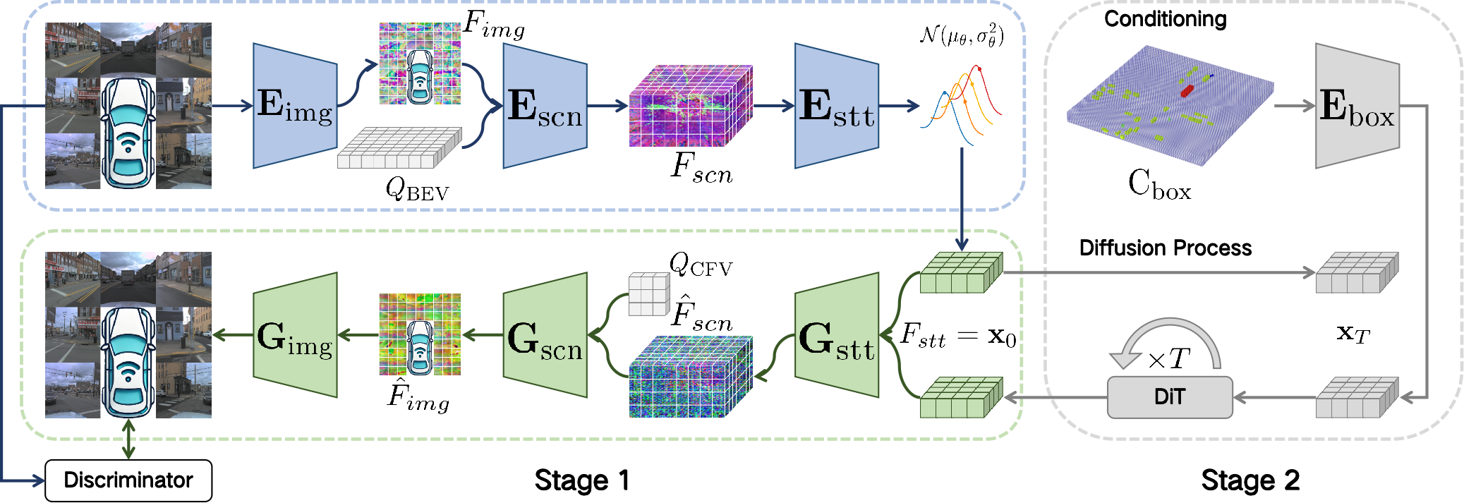
Training is split into a multi-view autoencoder stage and a latent generative stage. The architectural figure preserves both paths and their conditioning.
3.1 Overall Architecture
The encoder processes images, assembles multi-height scene features and compresses them into a sampled state latent. The decoder reverses this process through state, scene and image modules. A StyleGAN discriminator supplies an adversarial training signal alongside reconstruction and KL terms. The second-stage DiT generates in the learned scene space; it is not a temporally predictive driving policy.
3.2 Encoder
A ViT uses 8×8 patches on each 256×256 image, producing a 32×32 token grid. An upsampling-only three-level FPN supplies image features with 96 channels [23]. The scene encoder places eight height samples at each position of a 128×128 BEV grid, projects them with known camera calibration and gathers features only from views containing the projected points.
Queries share parameters along a pillar, with height positional encodings distinguishing samples. The state encoder concatenates eight heights into 768 channels, reduces the horizontal grid to 32×32 and applies self-attention. The resulting latent has d channels, evaluated at 4, 8, 16 and 32. Eight here counts height samples; the paper does not specify that the vertical extent is eight meters. The original feature aggregation and sequence-length definitions follow, with V denoting camera views and L sequence lengths.
Equations
3.3 Decoder
The state decoder expands 32×32 features to a 128×128 grid, splits channels into eight height levels, and builds a downsampled scene pyramid. For each camera, the scene decoder samples 60 depths on each of 32×32 rays and aggregates scene features with learned depth weights. Samples outside the represented scene receive zero weight. Camera parameters determine the mapping between frustum and BEV coordinates.
The image decoder maps the 96-channel features to width 768, adds interactions between rays with self-attention, and upsamples to 256×256 RGB. This is learned feature aggregation, not an explicit guarantee of correct visibility, surface geometry or radiance. The source equations retain their original notation, including the argument written as x̂ in the state-decoder formula.
Equations
3.4 Loss
The posterior is regularized toward a standard Gaussian, and reparameterization permits gradient training. Reconstruction combines squared pixel error with squared VGG-16 feature differences. A hinge discriminator loss separates real and reconstructed images; the generator receives the negative discriminator score. The total encoder/decoder objective uses β=10⁻⁶ and adversarial coefficient 0.1λ, with δ=10⁻⁶ in the adaptive gradient ratio.
All seven original definitions follow. The printed λ expression divides gradients and does not state a norm or scalar reduction convention; practical reproduction should check the implementation instead of assuming a missing operation. The small KL coefficient is a chosen regularization weight, not evidence that the learned posterior exactly matches the sampling prior.
Equations
3.5 Generation
Each box stores quaternion orientation, center, size and semantic class. Boxes become a class-specific binary occupancy tensor over eight heights and a 128×128 horizontal grid. Maximum occupancy merges overlapping boxes of the same class, so the condition does not retain separate instance identities. Patch processing produces a 768×32×32 conditional feature added to a corresponding state feature.
The main text writes a scale s on feature addition, while Appendix A also uses s in conventional classifier-free noise-prediction guidance. Both source formulas are retained; their shared symbol alone does not fully specify the implementation of guidance. The paper does not detail every projection between the d-channel VAE latent and the 768-channel conditioning representation.
Equations
4 Experiments
Experiments evaluate reconstruction and generation separately. The galleries preserve all cameras, editing examples and original captions, including examples where generated vehicle appearance changes.

4.1 Datasets
nuScenes supplies six cameras, 700 training and 150 validation scenes: 155,245 training samples and 33,142 validation samples, with 28,126 and 6,019 annotated samples respectively, across ten categories. AV2 supplies seven cameras and the same scene-split counts: 224,175 training and 47,946 validation samples, with 109,907 and 23,521 annotated samples, across 30 categories. The front AV2 camera uses a rotated orientation. Sample counts refer to synchronized multi-camera sets, not single images; labeled subsets are smaller than the complete image collections.
4.2 Metrics
PSNR and SSIM measure reconstruction against the input. FID measures feature-distribution differences for either reconstruction or generation; those two uses should not be compared as the same task. MVSC divides average LoFTR adjacent-view matching confidence by that of real images [24]. It is a relative feature-matching statistic, not a direct geometric error, a percentage of physically correct scenes or a guarantee of accurate layout adherence.
4.3 Settings
Training uses eight A800 GPUs and AdamW. The VAE stage runs 100,000 iterations at one sample per GPU, learning rate 4×10⁻⁵ on nuScenes or 8×10⁻⁵ on AV2, 5,000 warm-up steps, betas (0.9,0.99), weight decay 10⁻⁴ and EMA 0.9999.
The diffusion stage uses eight samples per GPU, learning rate 10⁻⁴, 400,000 iterations for nuScenes or 200,000 for AV2, 5,000 warm-up steps, betas (0.9,0.95), weight decay 0.1, zero bias decay and EMA 0.999. Wall-clock cost, sampling latency, repeated-seed uncertainty and several spatial-range/architecture details are not specified in the paper.
4.4 Reconstruction
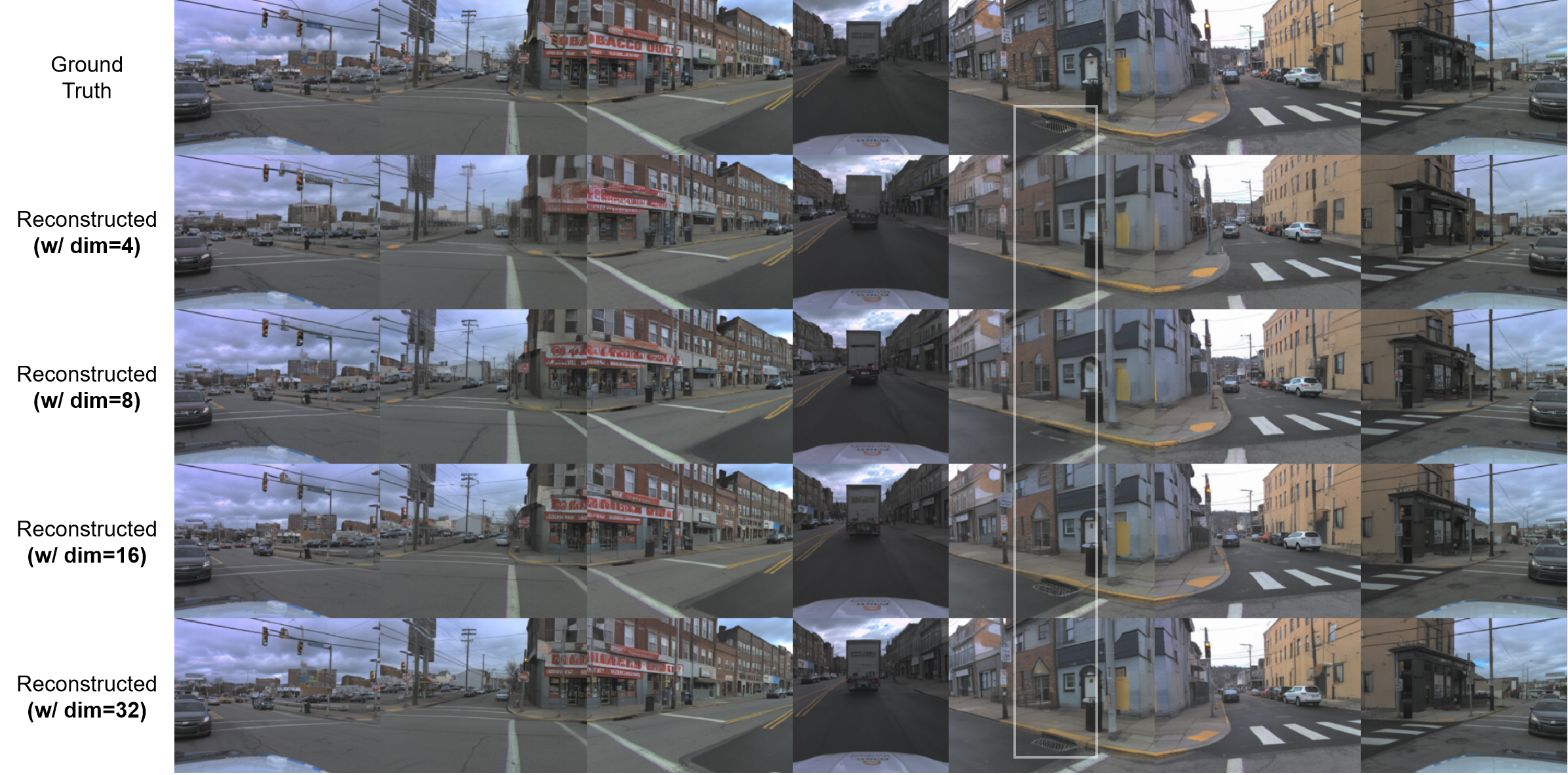
One 32×32×d latent represents the entire camera set, whereas the SD-VAE reference compresses each individual image into 32×32×4. Table 1 treats SD-VAE as a pretrained image-reconstruction reference, with substantially different training resources, rather than a controlled equal-budget baseline.
Larger d generally improves PSNR, SSIM and MVSC. On nuScenes, reconstruction FID improves to 11.42 at d=16 but worsens to 13.72 at d=32; suggested overfitting is not independently established. At d=32, AV2 reaches PSNR 26.68, SSIM 0.8004, MVSC 0.9505 and FID 3.02, compared with SD-VAE’s 27.81, 0.8229, 0.8962 and 1.87. Thus it improves this spatial-consistency proxy while remaining behind in per-image fidelity. On nuScenes its best listed MVSC 0.9291 is still just below SD-VAE’s 0.9292.
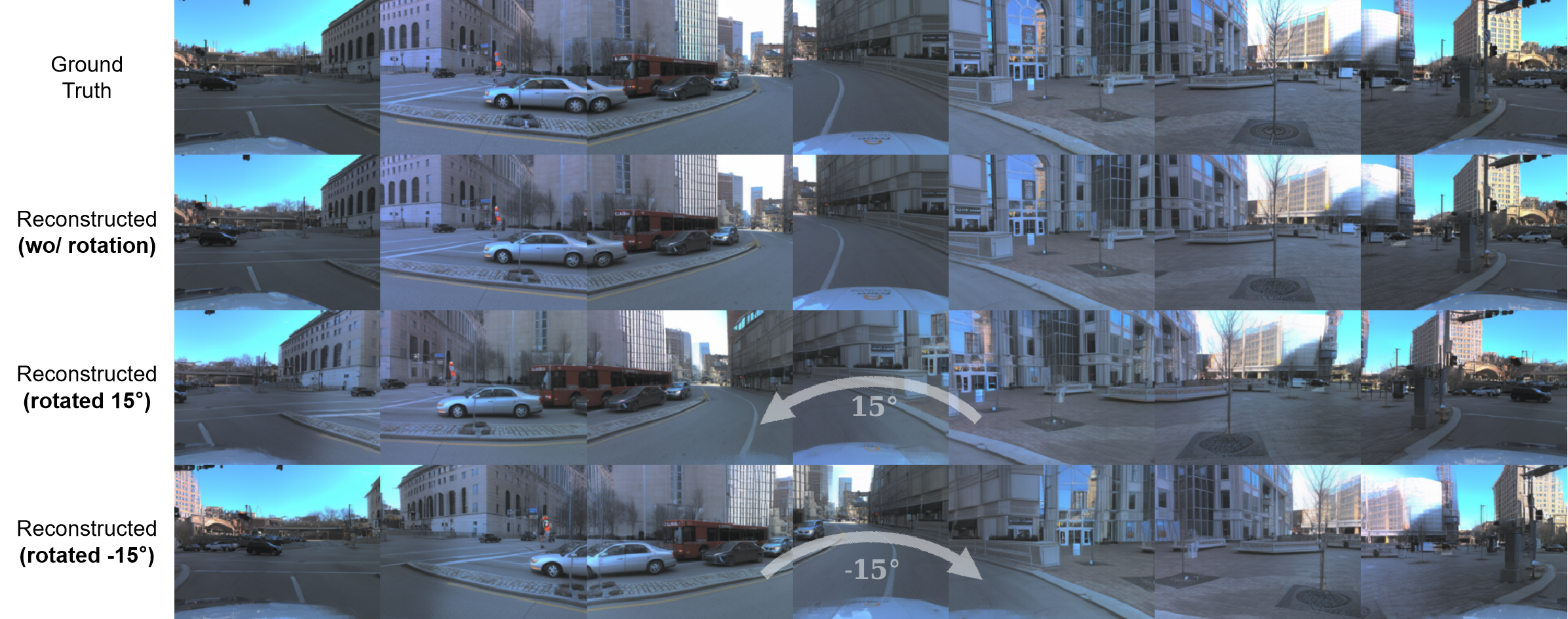
The camera-rotation galleries use d=32 and illustrate novel views around original poses. They do not include quantitative ground truth for newly synthesized viewpoints. Larger reconstruction capacity does not imply a better generative latent, as the next experiment shows.
4.5 Generation
The best generative latent in the reported sweep is d=8. nuScenes reaches FID 21.14 at guidance s=5; AV2 reaches 10.68 at s=3. Higher d makes reconstruction easier but makes modeling the latent distribution harder under the reported training setup.
On nuScenes, 21.14 improves on from-scratch BEVGen’s 25.54 but trails the listed Stable Diffusion-based results: Panacea 16.96, MagicDrive 16.20, DrivingDiffusion 15.83 and DriveWM 12.99. Similar absence of pretrained generative priors does not by itself equalize all resources or conditions. AV2 has no direct seven-view baseline here, and its lower FID than nuScenes cannot establish a scaling law because dataset content, cameras, labels and training iterations also differ.
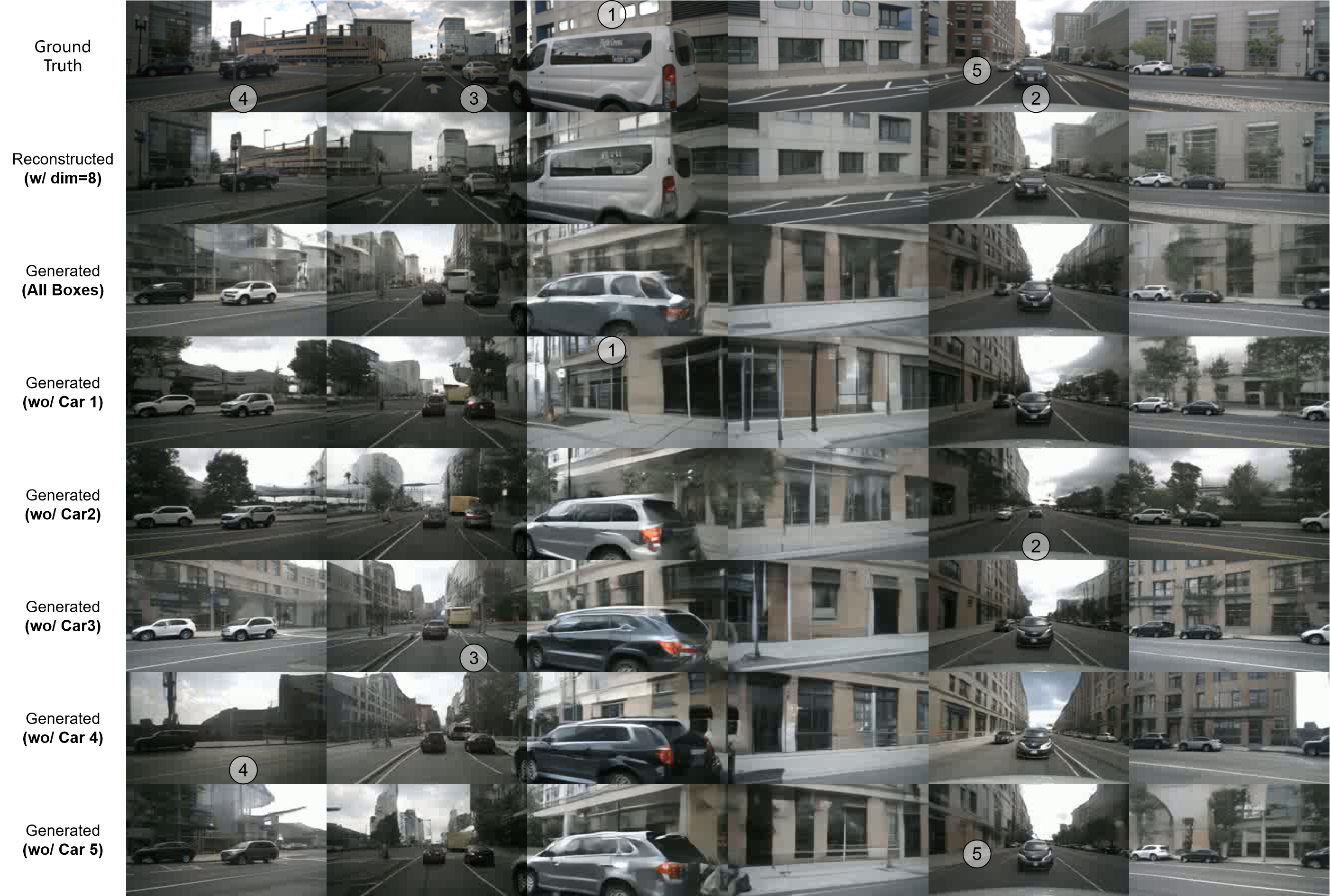
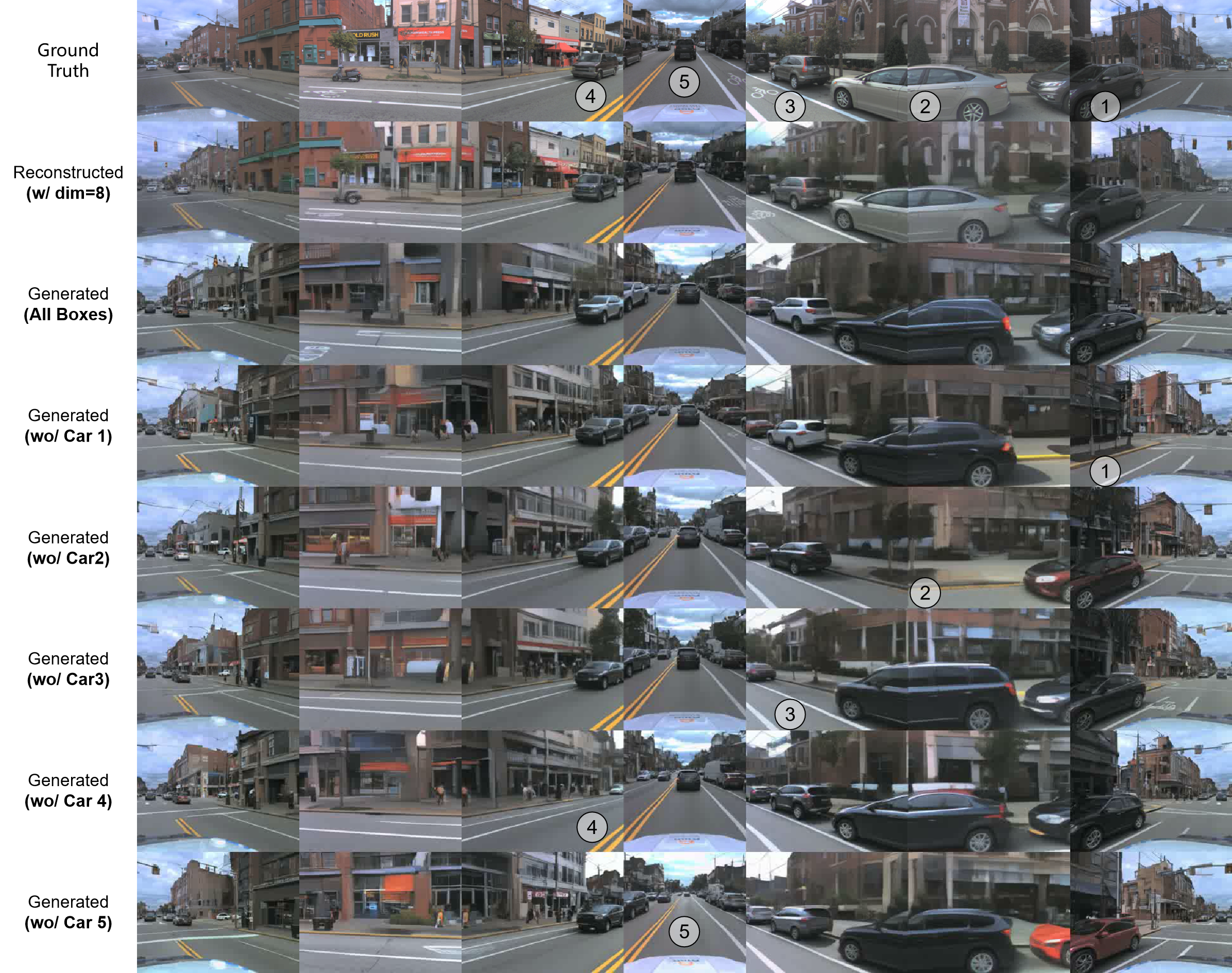
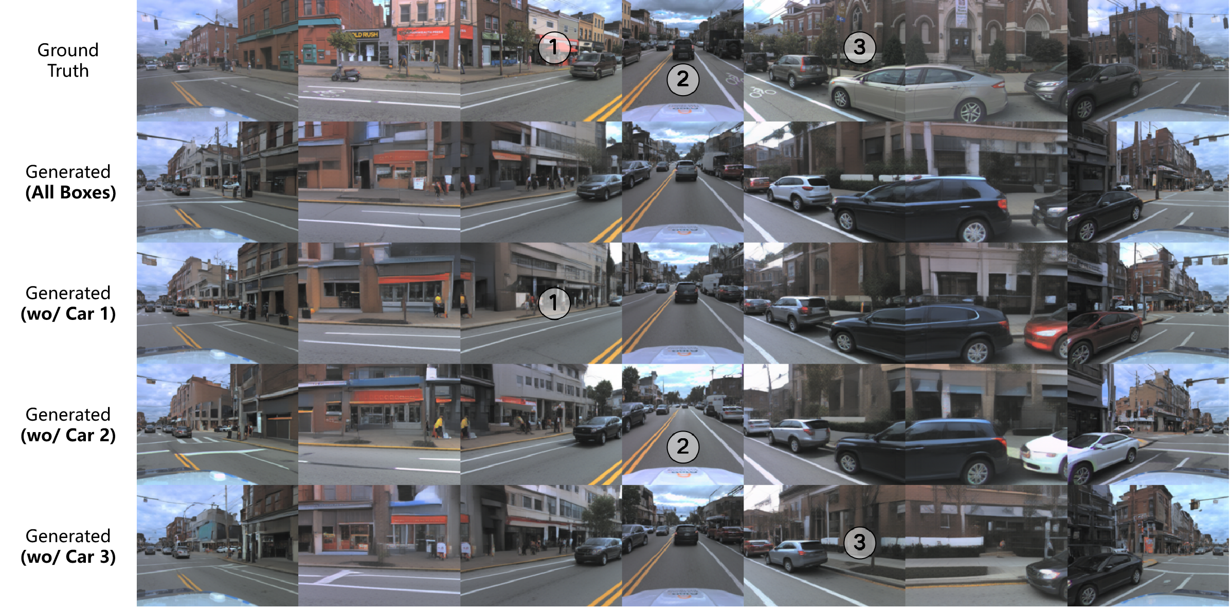
Object-removal examples show layout control qualitatively, with no numerical removal, box-adherence or identity-retention metric. The same box can produce different appearances across generated samples or views. The source cross-references around Tables 2–4 are imperfect; the original numbered table captions and panels are retained.
| Scale | ||||
|---|---|---|---|---|
| 30.04 | 32.01 | 40.31 | 47.10 | |
| 27.19 | 24.17 | 30.03 | 38.58 | |
| 24.14 | 22.43 | 24.63 | 32.78 | |
| 23.41 | 22.22 | 23.45 | 31.03 | |
| 22.94 | 22.11 | 23.42 | 30.31 | |
| 23.06 | 21.14 | 23.74 | 30.52 |
| Method | Paradigm | Extra Prior | FID |
|---|---|---|---|
| BEVGen | Autoregression | None | 25.54 |
| Panacea | Diffusion | Stable Diffusion | 16.96 |
| MagicDrive | Diffusion | Stable Diffusion | 16.20 |
| DrivingDiffusion | Diffusion | Stable Diffusion | 15.83 |
| DriveWM | Diffusion | Stable Diffusion | 12.99 |
| BEV-VAE w/ DiT | Diffusion | None | 21.14 |
4.6 Analysis of Loss Function
The AV2 d=8 loss ablation gives reconstruction FID 5.10 with the full objective, 68.99 without perceptual loss, 13.62 without adversarial loss, and 8.09 when replacing squared error with L1. The full objective’s PSNR/SSIM/MVSC are 24.02/0.6870/0.8827. Removing the adversarial term raises MVSC to 0.9053 and PSNR to 24.87, illustrating a fidelity/consistency trade-off rather than uniform improvement across metrics. These are single reported configurations without confidence intervals.
5 Conclusion
A structured scene latent enables shared-coordinate image decoding and useful qualitative control. The evidence supports a representation and generative-model design, while leaving high-resolution fidelity, temporal coherence, physical correctness, cross-dataset transfer and downstream driving benefit unresolved. Temporal models and physical priors are future directions rather than tested capabilities.
Appendix A Preliminary for Generative Models
The eight original equations cover the VAE evidence lower bound, Gaussian forward diffusion, reparameterization, the reverse process, noise-prediction loss and classifier-free guidance. The VAE maximizes its ELBO, equivalently minimizing the negative bound; the source’s later phrase about minimizing the ELBO should be interpreted with that sign distinction. Conditioning dropout trains both conditional and unconditional predictions. The final guidance relation is schematic, so its proportionality should not be read as a fully specified equality without the appropriate score/noise scaling.
Equations 1–8
| (1) |
| (2) |
| (3) |
| (4) |
| (5) |
| (6) |
| (7) |
| (8) |
Appendix B Evaluation with Multi-View Spatial Consistency
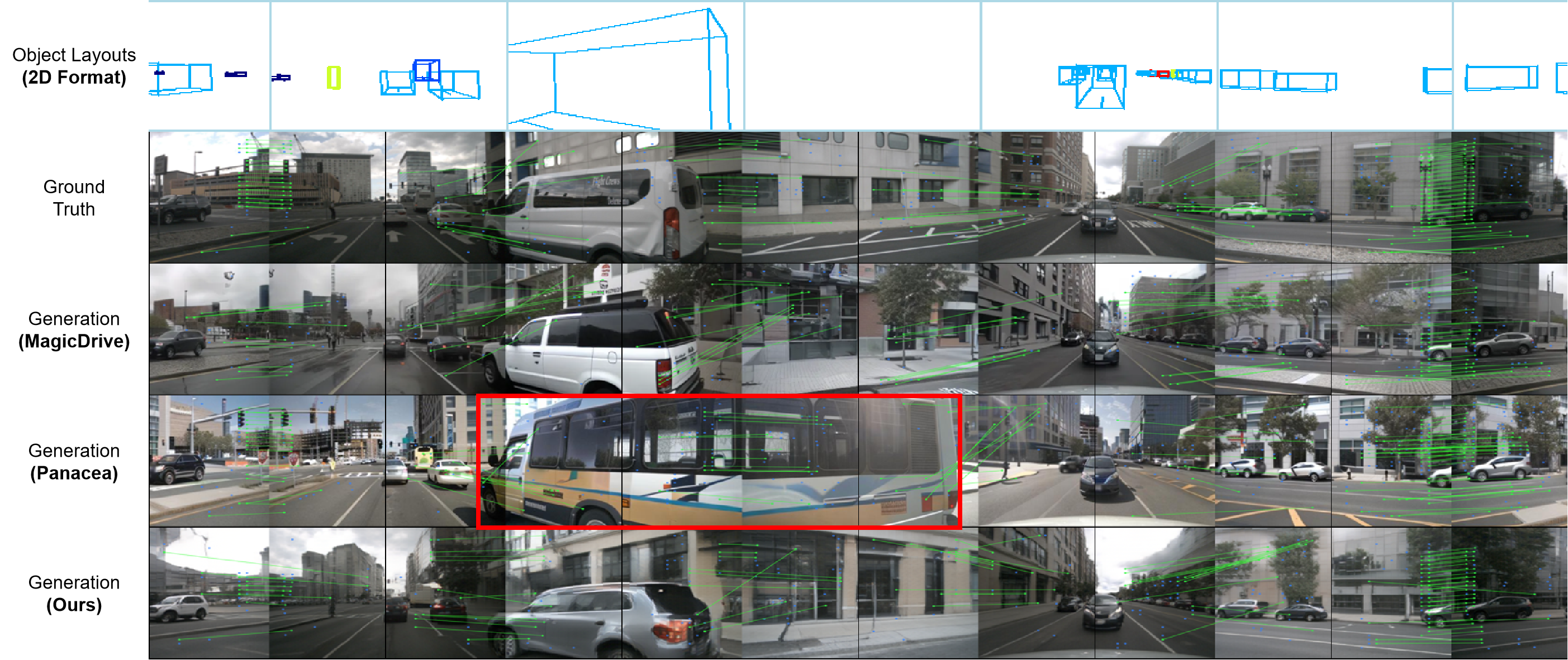
LoFTR matches the bordering half-images of each adjacent camera pair; MVSC is the mean confidence relative to real-image matches. The source calls it both Multi-View Spatial Consistency and Multi-View Spatial Confidence. Neither name changes the measured quantity. The appendix comparison reports MagicDrive 0.8310, Panacea 0.9189 and BEV-VAE 0.8902; BEV-VAE is between the two and has worse FID than both.
Panacea also uses text, map and depth conditions, and MagicDrive uses text and maps; BEV-VAE uses 3D occupancy plus extrinsics. The highlighted misaligned vehicle in Figure 7 illustrates that matching confidence need not imply agreement with the intended boxes. The paper’s explanation that extra conditioning partly causes Panacea’s higher score is not isolated by an ablation.
| Method | FID | MVSC | Object Layouts | Camera Poses | Other Conditions |
|---|---|---|---|---|---|
| MagicDrive | 16.20 | 0.8310 | Fourier embedding(1D) | Fourier embedding | Text, map. |
| Panacea | 16.96 | 0.9189 | Perspective projection (2D) | Pseudo-color image | Text, map, depth. |
| Ours | 21.14 | 0.8902 | Binary occupancy (3D) | Extrinsic matrix | None |
Appendix C Reconstruction with Camera Pose Control
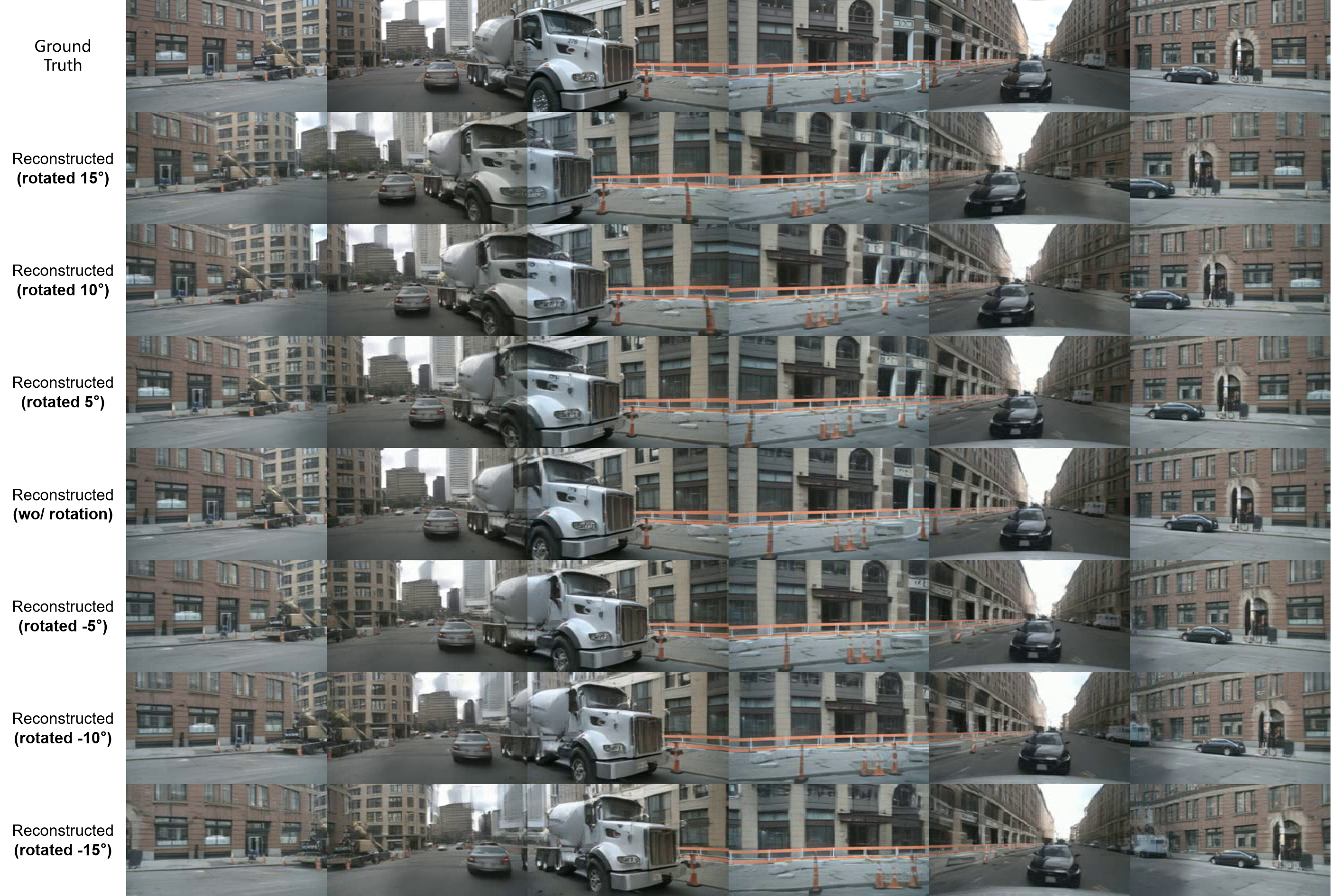
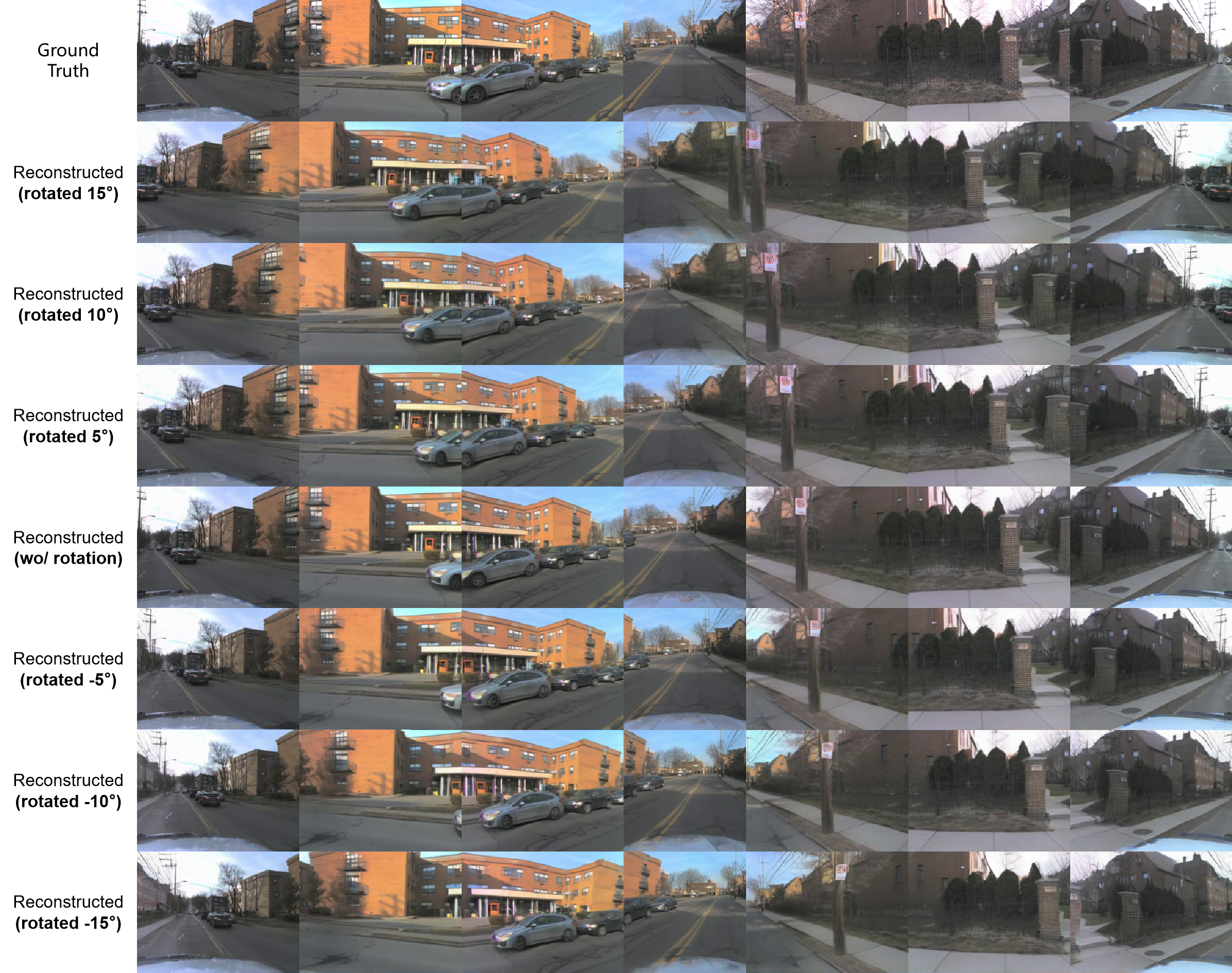
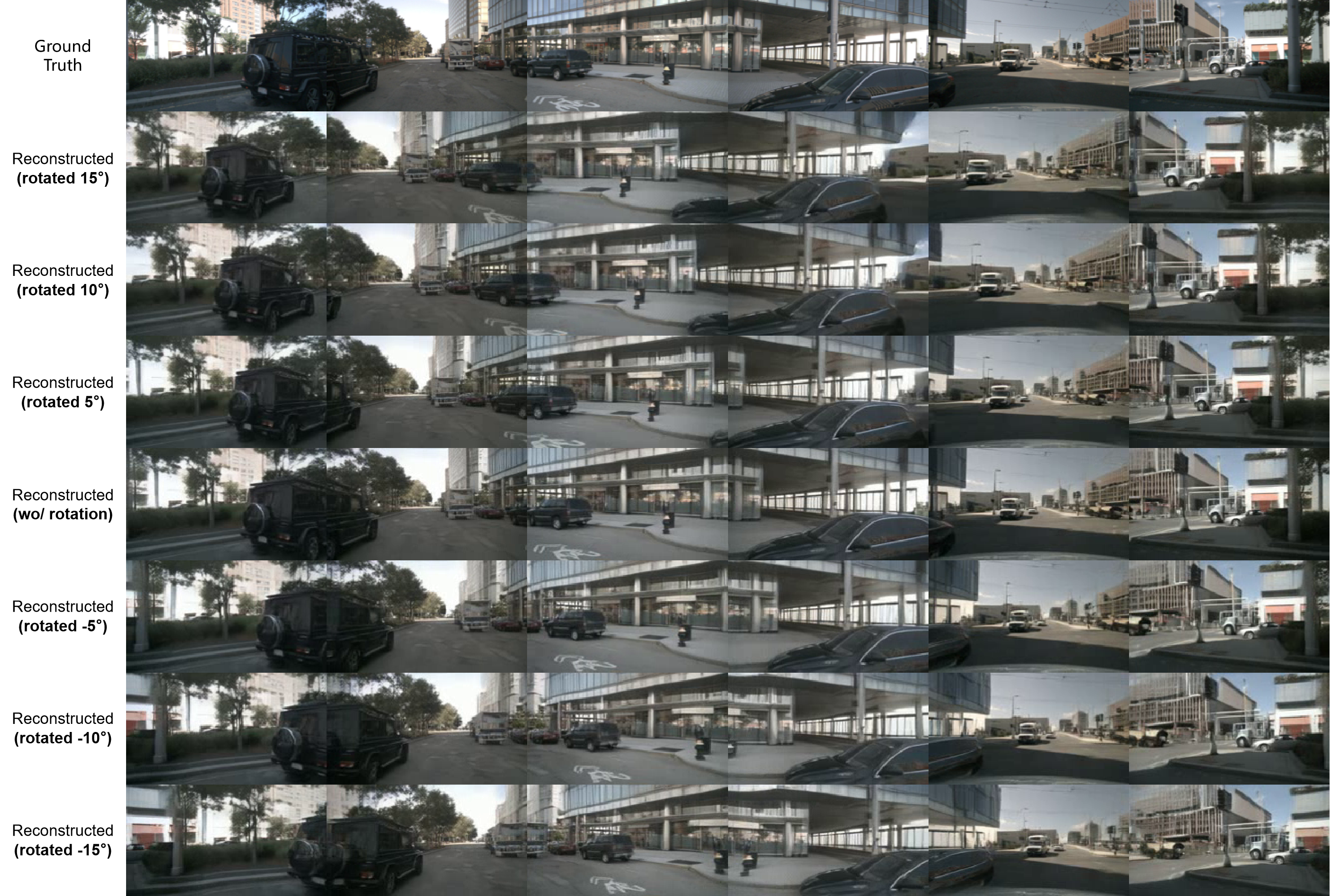
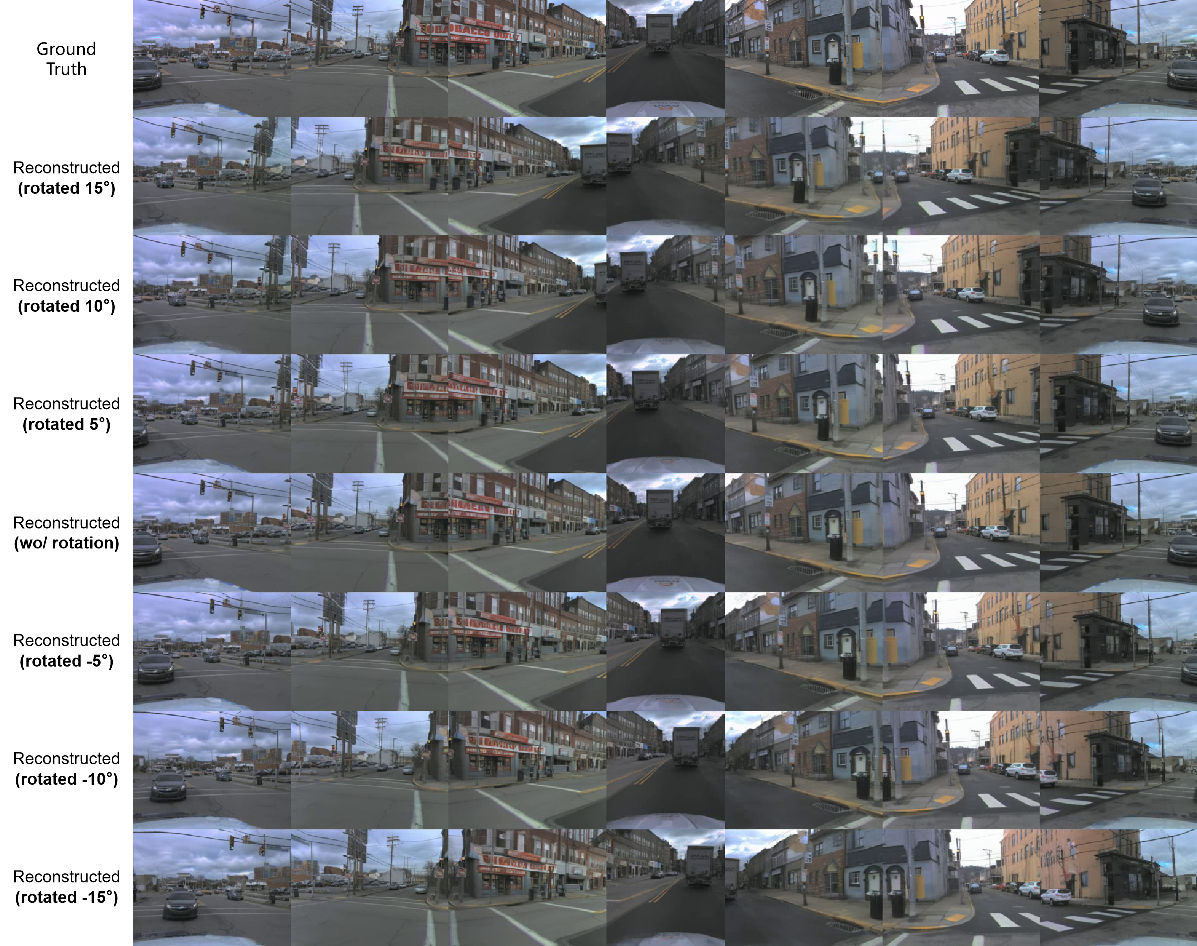
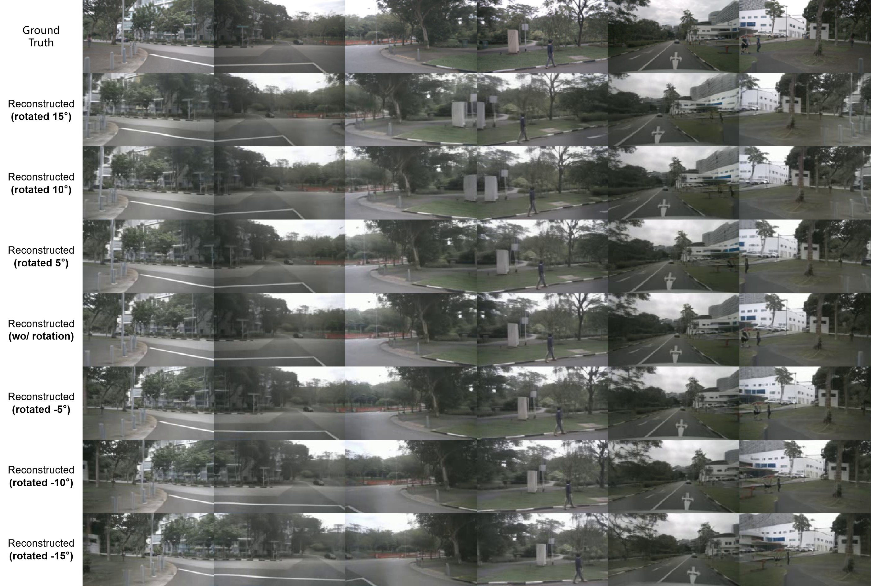
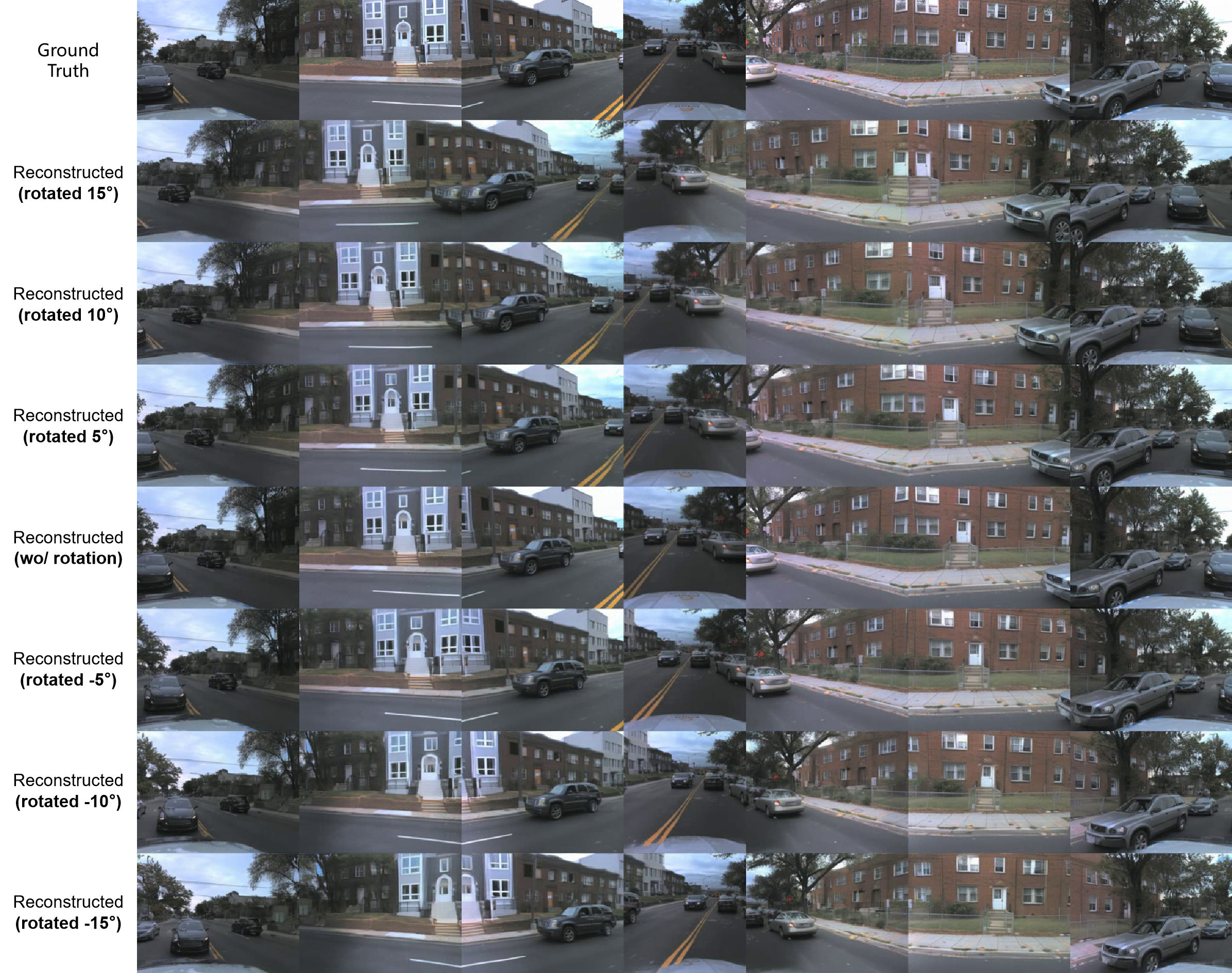
Figures 8–13 preserve three scenes from each dataset. Each has the original camera images plus seven reconstructed rows at +15°, +10°, +5°, 0°, −5°, −10° and −15°, using d=32. They demonstrate modest rotation control from an encoded scene, not unrestricted camera translation or guaranteed reconstruction of previously unseen surfaces.
Appendix D Generation with Precise 3D Object Control
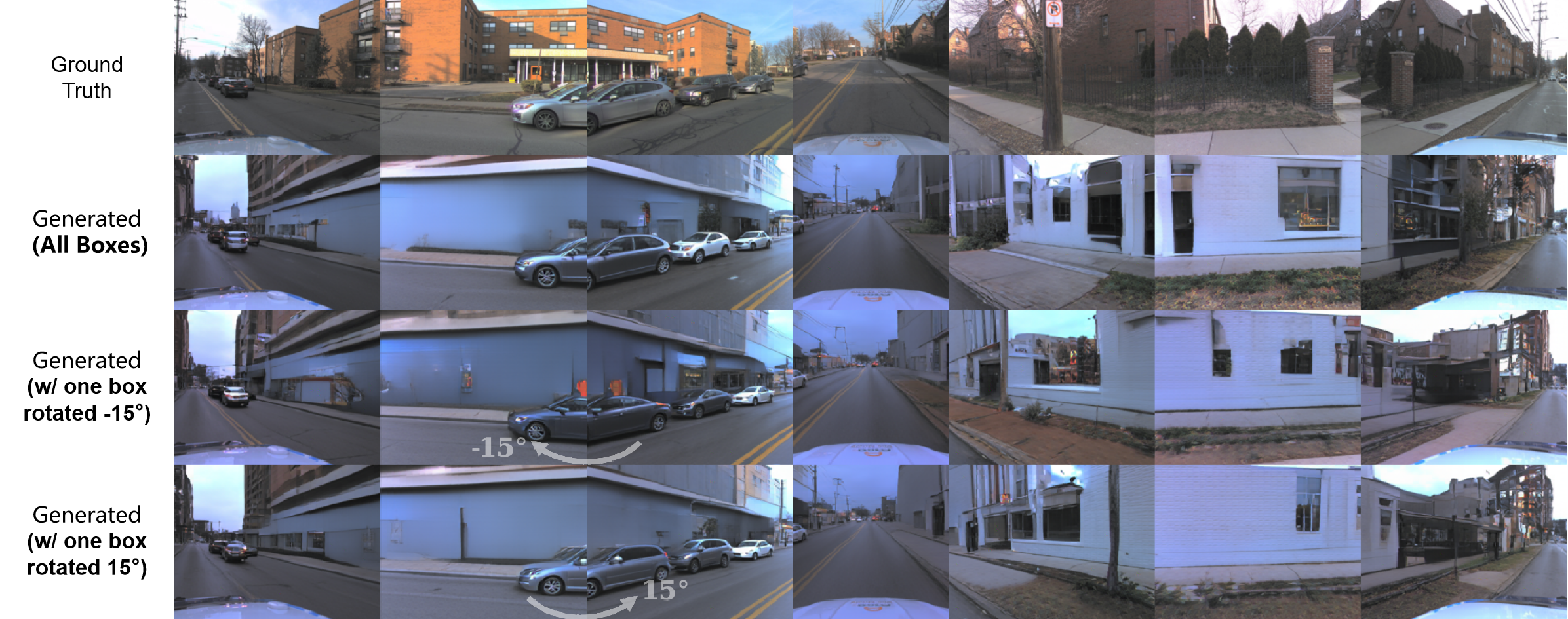
Figures 14–15 retain the real images, reconstruction, generation from all boxes and five separate vehicle-removal settings. Figure 16 rotates one vehicle’s box ±15° on the ego horizontal plane. These are selected visual demonstrations; the paper reports no aggregate edit-success rate. Appearance may change even when a box is unchanged, so occupancy control does not imply persistent vehicle identity.
Appendix E Limitations in Resolution and Data Scale
The authors acknowledge blur, 256×256 resolution and limited training data, especially on nuScenes. They attribute limitations to data scale and lack of pretrained image priors, but do not separately rule out architecture or optimization constraints. AV2 is about 1.44 times as large by the exact unannotated training-sample counts, described approximately as 1.5×. Better AV2 results are suggestive, not a controlled scaling experiment. All supplementary gallery panels remain below, including full labels supplied by the native images where the PDF page margin clips them.