At a glance
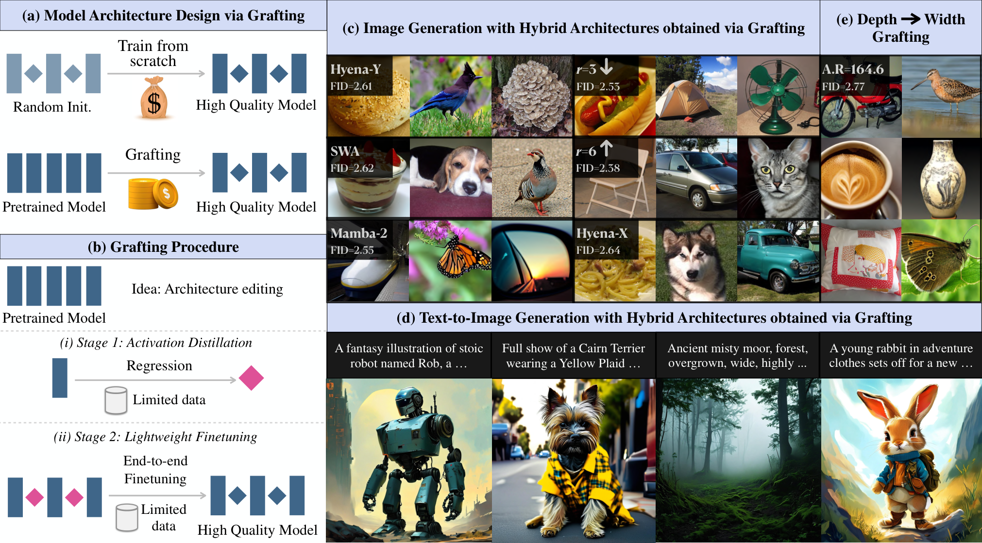
Grafting studies new diffusion-transformer architectures by editing pretrained models. It first trains replacement operators to match intermediate activations, then fine-tunes the assembled model to repair accumulated errors. Interleaved attention replacements, altered feed-forward widths and parallelized transformer blocks preserve much of the original image quality with limited additional training. The method measures compatibility with an existing pretrained model; whether the resulting architecture would train equally well from scratch remains unresolved.
1 Introduction
Architecture experiments are expensive when each candidate must be pretrained. Grafting treats a pretrained diffusion transformer [1] as a reusable starting point. Its two problems are initializing a replacement operator and preventing errors from compounding when many replacements are combined. It explores which operator to replace, its alternative, the selected layers and the replacement fraction.
The main evidence covers ImageNet class-conditional generation with DiT-XL/2, high-resolution text-to-image generation with PixArt-Σ [11], and a depth-to-width restructuring case. Several hybrid variants retain low FID after a small adaptation budget. These are incremental costs on top of existing pretraining, not equivalent costs for training a new model from no checkpoint.
2 Prerequisites
Latent diffusion adds time-dependent Gaussian noise to an encoded image and trains a denoiser conditioned on a class or text prompt. DiT processes patchified noisy latents using attention and feed-forward blocks. The original denoising objective remains available.
ImageNet evaluation generates 50,000 samples with 250-step DDPM sampling and classifier-free guidance 1.5, reporting FID, spatial FID, Inception Score, precision and recall. Text-to-image quality uses GenEval [16]. Low FID and high GenEval measure different aspects of generated distributions and prompt alignment; neither alone establishes visual fidelity on every image.
Equation 1
| (1) | ||||
3 Grafting Diffusion Transformers
The two stages separately address operator initialization and whole-model recovery. Self-grafting is the control that preserves the architecture while replacing operator weights.
3.1 Two - Stage Grafting Approach
Activation distillation trains each replacement to reproduce its pretrained operator’s outputs under noisy inputs and conditioning. The regression loss compares teacher and student intermediate tensors, using around 8,000 training examples. This borrows the teacher’s behavior rather than deriving a new architecture objective from scratch.
After insertion, small operator errors can accumulate through the network. End-to-end fine-tuning with the ordinary denoising objective repairs this mismatch, commonly using 10% of ImageNet. Success therefore depends on both local imitation and global adaptation; a low isolated activation loss does not guarantee a usable assembled generator.
Equation 2
| (2) |
(iii) MHA initialization
| IS | FID | sFID | Prec. | Rec. | |
| Baseline | 278.20 | 2.27 | 4.60 | 0.83 | 0.57 |
| Random Init. | 40.86 | 76.27 | 10.33 | 0.33 | 0.52 |
| L2 | 269.31 | 2.58 | 5.75 | 0.82 | 0.58 |
| Huber (=1.0) | 271.30 | 2.55 | 5.44 | 0.82 | 0.57 |
| L1 | 273.03 | 2.51 | 5.48 | 0.83 | 0.58 |
(iv) MLP initialization
| IS | FID | sFID | Prec. | Rec. | |
| Baseline | 278.20 | 2.27 | 4.60 | 0.83 | 0.57 |
| Random Init. | 2.18 | 297.34 | 161.76 | 0.01 | 0.00 |
| L2 | 265.34 | 2.33 | 4.38 | 0.81 | 0.59 |
| Huber (=1.0) | 262.93 | 2.38 | 4.49 | 0.81 | 0.59 |
| L1 | 235.54 | 2.83 | 4.69 | 0.77 | 0.61 |
3.2 Self - grafting Baseline
Self-grafting swaps attention or MLP operators for randomly initialized copies with identical shapes, receptive fields and parameter counts. It isolates the recovery procedure from changes in architecture. Its near-baseline results are evidence that the initialization/fine-tuning pipeline works, not evidence that attention can be removed without recovery.
3.3 Activation Behavior Analysis and Self-grafting Results
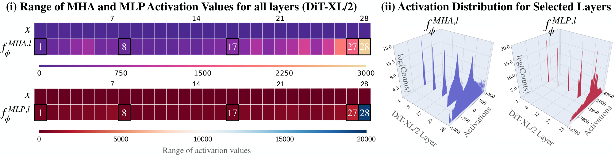
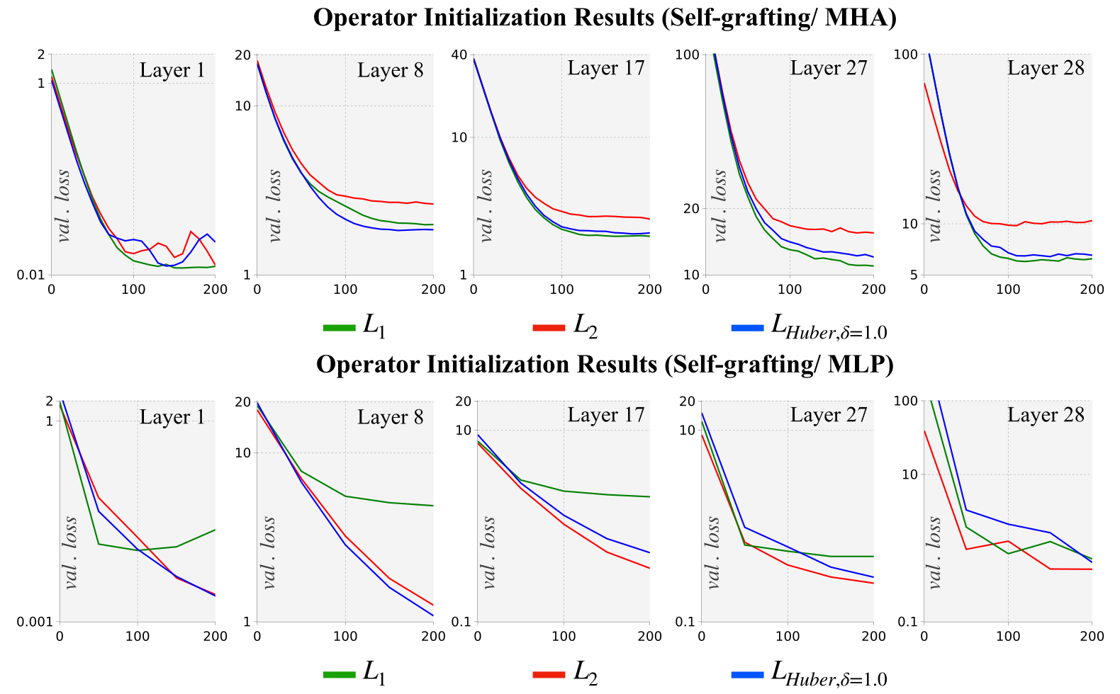
Activation ranges vary substantially across layers, especially in deeper MLPs. In five selected layers, L1 distillation yields attention FID 2.51 versus 2.58 for L2 and 2.55 for Huber. MLPs favor L2: 2.33 versus 2.38 for Huber and 2.83 for L1. The authors attribute this difference partly to MLPs having twice as many parameters, but no capacity-controlled experiment isolates that explanation.
Full attention self-grafting is poor immediately after initialization: Table 2 gives FID 16.78 with 8K distillation examples and no final adaptation. With 128K fine-tuning examples it recovers to 2.49, compared with the original 2.27; full MLP self-grafting reaches 2.54. The paragraph says 2.53 for attention, but Table 2 and subsequent plots use 2.49. Both source values are preserved, and the table is used for the numerical comparison here.
| Stage 1 | Stage 2 | IS | FID | sFID | Prec. | Rec. |
| Baseline | 278.20 | 2.27 | 4.60 | 0.83 | 0.57 | |
| MHA (Full Self-grafting) | ||||||
| Random Init. | 1.66 | 289.23 | 154.00 | 0.00 | 0.00 | |
| 0.63% | – | 117.68 | 16.78 | 13.69 | 0.60 | 0.61 |
| 0.63% | 0.63% | 148.56 | 11.26 | 11.10 | 0.66 | 0.60 |
| 0.63% | 5.0% | 270.39 | 2.70 | 5.46 | 0.81 | 0.57 |
| 0.63% | 10.0% | 287.81 | 2.49 | 4.71 | 0.83 | 0.56 |
| MLP (Full Self-grafting) | ||||||
| Random Init. | 1.27 | 314.72 | 204.99 | 0.00 | 0.00 | |
| 0.63% | 10.0% | 277.72 | 2.54 | 4.52 | 0.83 | 0.57 |
3.4 Locality Analysis of Self-attention
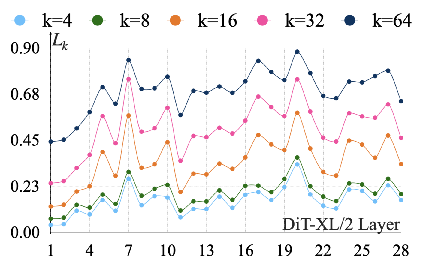
The band-k metric measures attention mass within k positions on either side in the flattened token sequence. It averages 250 generated samples, diffusion timesteps and attention patterns; at k = 32, 15 of 28 layers put more than half their mass locally. Early layers are less local. This is sequence-index locality, not necessarily a uniform two-dimensional image neighborhood.
Local mass guides replacement but is not a proof that distant interactions are dispensable. Directly replacing all attention with sliding-window attention gives FID 53.9, and full replacement remains poor in the grafting experiments. Interleaving preserves some global attention and generally works better than indiscriminate substitution.
Equations 3
| (3) |
4 Experiments I: Hybrid Architectures via Grafting
The ImageNet testbed compares attention alternatives and feed-forward alternatives under full or interleaved replacement. All configurations and numerical outcomes are retained in restored semantic tables.
4.1 Testbed and Experiment setup
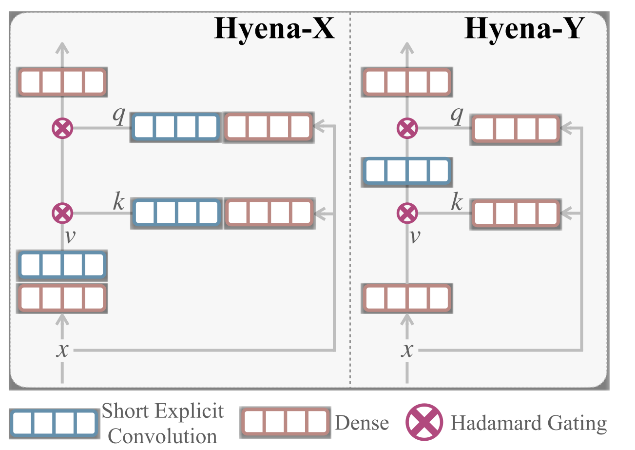
Attention alternatives include sliding-window attention [26], Mamba-2 [28] and local gated convolutions. Hyena-X removes the long implicit convolution from a Hyena-style operator [52]; Hyena-Y instead removes the three featurizer convolutions and keeps a short inner filter. Both use dense projections plus local mixing. Hyena-X also supplies an MLP alternative that mixes channels.
Stage 1 independently fits replacement operators on 8K examples for 200 epochs, batch 64, with pre-extracted features. The main text specifies learning rate 10⁻⁴; Appendix Table B.1 says 10⁻³, an unresolved recipe discrepancy. Stage 2 usually uses 128K examples, 50K updates, batch 256 and learning rate 10⁻⁴ after 1K warmup steps. Reported standard runs take under ten hours on eight H100 GPUs, with larger ablations up to 24 hours. Feature extraction and all previous model pretraining should be considered when interpreting incremental compute savings.
| Operator Type: Which operator types are we replacing? | ||
| MHA, MLP | ||
| Efficient Alternative: What do we replace it with? | ||
| MHA | Convolutions: Hyena-SE [24], Hyena-X/ Hyena-Y (Ours) | =4, causal |
| Local Attention: Sliding Window Attention (SWA) [26, 27] | =4, bidirectional | |
| Linear Attention: Mamba-2 [28] | =64, =2 | |
| MLP | Variable expansion ratio | =3,6 |
| Hyena-X (Ours) | =2, =4, causal, mix channels | |
| Layer Selection: In which layers is the operator replaced? | ||
| Full | Replace the operator in all layers | |
| Interleaved | Replace the operator in a repeating pattern (e.g., every 2 or 3 out of 4) | |
| Replacement Ratio: What percentage of operators are replaced? | ||
| 50%, 75%, 100% | ||
4.2 Results and Insights
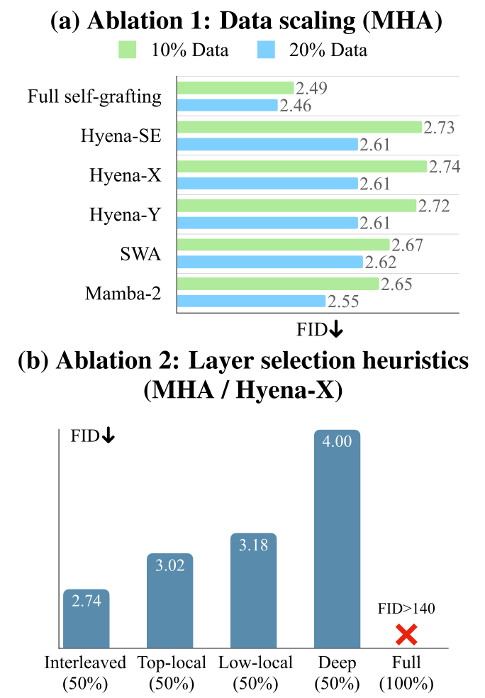
At 50% attention replacement, standard 10%-data results remain within about 0.5 FID of the 2.27 baseline: Hyena-SE 2.73, Hyena-X 2.74, Hyena-Y 2.72, sliding-window attention 2.67 and Mamba-2 2.65. Increasing replacement to 75% generally hurts; sliding-window attention is still 3.09. Full replacement fails badly. Expanding fine-tuning data to 20% improves the 50% variants, including Hyena-X to 2.61 and Mamba-2 to 2.55. The headline range combines selected settings rather than describing every standard configuration.
For Hyena-X, interleaving gives 2.74, selecting the most local layers 3.02, the least local 3.18 and the deepest layers 4.00. The locality score has some predictive value, yet interleaving beats it. Feed-forward width changes tolerate even full replacement: expansion ratio three reaches 2.66, while wider ratio-six variants retain strong quality but increase parameters and FLOPs. The convolutional MLP alternative degrades more at high replacement fractions.
Table 4 separates operator mixing from projections/featurizers. A roughly 50% reduction in the attention-mixing component is not a 50% reduction in whole-model work. At 50% Mamba-2 replacement, mixing FLOPs fall 37.59% while projection/featurizer FLOPs rise 77.89% and operator parameters rise 28.02%. Wider MLPs also deliberately spend more computation. These distinctions prevent treating every grafted variant as a smaller or faster model.
| Ratio | IS | FID | sFID | Prec. | Rec. | FLOPsop. | FLOPsft. | Param | |
| Baseline | – | 278.20 | 2.27 | 4.60 | 0.83 | 0.57 | — | — | — |
| MHA Grafting | |||||||||
| Random Init. | 100% | 1.66 | 289.23 | 154.00 | 0.00 | 0.00 | — | — | — |
| Self-grafting | 100% | 287.81 | 2.49 | 4.71 | 0.83 | 0.56 | — | — | — |
|
(=4)
|
50% | 274.73 | 2.73 | 5.05 | 0.82 | 0.56 | -49.52% | +0.13% | +0.22% |
| 75% | 231.15 | 3.62 | 6.04 | 0.81 | 0.54 | -74.27% | +0.20% | +0.33% | |
| 100% | ✗ | ✗ | ✗ | ✗ | ✗ | -99.03% | +0.26% | +0.43% | |
|
(=4)
|
50% | 273.30 | 2.74 | 5.03 | 0.83 | 0.56 | -49.90% | +0.13% | +0.16% |
| 75% | 229.11 | 3.69 | 6.10 | 0.81 | 0.53 | -74.85% | +0.20% | +0.24% | |
| 100% | ✗ | ✗ | ✗ | ✗ | ✗ | -99.81% | +0.26% | +0.33% | |
|
(=4)
|
50% | 273.37 | 2.72 | 5.02 | 0.83 | 0.55 | -49.52% | 0.00% | +0.05% |
| 75% | 228.99 | 3.66 | 5.95 | 0.81 | 0.53 | -74.27% | 0.00% | +0.08% | |
| 100% | ✗ | ✗ | ✗ | ✗ | ✗ | -99.03% | 0.00% | +0.11% | |
|
(=4)
|
50% | 280.62 | 2.67 | 4.90 | 0.83 | 0.56 | -48.24% | 0.00% | 0.00% |
| 75% | 249.99 | 3.09 | 5.54 | 0.82 | 0.55 | -72.36% | 0.00% | 0.00% | |
| 100% | ✗ | ✗ | ✗ | ✗ | ✗ | -96.48% | 0.00% | 0.00% | |
|
(=64, =2)
|
50% | 285.08 | 2.65 | 4.84 | 0.83 | 0.55 | -37.59% | +77.89% | +28.02% |
| 75% | 257.66 | 3.02 | 5.48 | 0.82 | 0.53 | -56.38% | +116.83% | +42.04% | |
| 100% | ✗ | ✗ | ✗ | ✗ | ✗ | -75.17% | +155.77% | +56.05% | |
| MLP Grafting | |||||||||
| Random Init. | 100% | 1.27 | 314.72 | 204.99 | 0.00 | 0.00 | — | — | — |
| Self-grafting | 100% | 277.72 | 2.54 | 4.52 | 0.83 | 0.57 | — | — | — |
|
Exp. ratio
(=3)
|
50% | 272.14 | 2.53 | 4.51 | 0.83 | 0.57 | -12.50% | 0.00% | -12.50% |
| 75% | 279.72 | 2.61 | 4.61 | 0.83 | 0.56 | -18.75% | 0.00% | -18.75% | |
| 100% | 252.11 | 2.66 | 4.57 | 0.81 | 0.57 | -25.00% | 0.00% | -25.00% | |
|
Exp. ratio
(=6)
|
50% | 278.00 | 2.38 | 4.50 | 0.83 | 0.58 | +25.00% | 0.00% | +25.00% |
| 75% | 277.94 | 2.37 | 4.48 | 0.82 | 0.58 | +37.50% | 0.00% | +37.50% | |
| 100% | 276.86 | 2.42 | 4.50 | 0.82 | 0.58 | +50.00% | 0.00% | +50.00% | |
|
(=2,=4)
|
50% | 265.60 | 2.64 | 4.66 | 0.83 | 0.56 | +0.01% | 0.00% | +0.02% |
| 75% | 226.13 | 3.26 | 4.79 | 0.81 | 0.55 | +0.02% | 0.00% | +0.03% | |
| 100% | ✗ | ✗ | ✗ | ✗ | ✗ | +0.02% | 0.00% | +0.03% | |
5 Experiments II: Grafting Text-to-Image Diffusion Transformers
PixArt-Σ generates 2048×2048 images with 16,384 tokens. Attention consumes over 62% of its measured generation latency, motivating Hyena-X replacement. A small synthetic dataset contains 12K uncurated image-text pairs, with prompts sampled from the model’s public 30K evaluation prompt set. Stage 1 uses 8K pairs and L1 distillation; Stage 2 uses rank-64 LoRA [29] on the full synthetic set. Generation uses a 20-step DPM solver [30].
The 50% variant replaces layers 8, 10, 12, 14, 16, 18 and 20–27, a mixture of interleaved and contiguous late layers. Its GenEval score falls from 49.75 to 47.78: 1.97 percentage points, approximately 3.96% relative. The abstract’s “less than 2%” should be read as a point difference, not a relative percentage. Counts and positions improve slightly while several color and object-related scores decline.
Single-forward-pass latency on one H100 at batch two falls from 235.46 to 164.58 ms, a 1.43× speed ratio or about 30% less latency. This table does not measure end-to-end prompt-to-image wall time including every sampling and decoding step. The 29% variant gives 48.04 GenEval and 194.95 ms. Failure examples reveal incorrect counts, malformed structure and inherited synthetic-data artifacts; LoRA capacity is a proposed explanation, not an isolated causal result.
| Model | Ratio | Obj(1) | Obj(2) | Count | Colors | Pos | Color Attr. | Overall | Latency (ms) |
| Baseline | - | 81.45 | 61.62 | 46.25 | 77.13 | 10.75 | 21.50 | 49.75 | 235.46 |
| Hyena-X | 29% | 80.31 | 59.34 | 49.69 | 68.62 | 11.50 | 18.75 | 48.04 | 194.95 (1.21) |
| Hyena-X | 50% | 80.00 | 57.07 | 48.13 | 70.74 | 11.25 | 19.50 | 47.78 | 164.58 (1.43) |
6 Case Study: Converting Model Depth to Width via Grafting
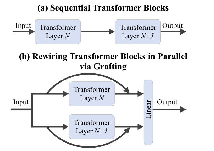
The depth-to-width case sends the same input through two formerly sequential transformer blocks, then combines outputs with a linear projection. The 28-block model becomes 14 parallel pairs, retaining both branches and adding projection parameters. It is shallower in sequential computation, not a halving of the model’s parameters: the total rises from 675M to 712M.
Unlike random self-grafting, each branch begins from its corresponding pretrained block. L1 activation matching uses 8K examples; recovery uses 320K examples, 25% of ImageNet, for up to 230K steps. FID is 3.12 at 100K updates and 2.77 at 230K, compared with the original 2.27. The longer case has a different budget from the standard 50K-step hybrid experiments.
At 14 sequential stages, 2.77 beats TinyDiT with masked distillation at 2.86 and other reported shallow baselines, but the grafted model has 712M parameters versus 340M for the pruning baselines. Its spatial FID 4.87 is worse than TinyDiT’s 4.75. Reported 2× speed uses a fused implementation and one H100 forward pass at batch two; quality uses the exact illustrated implementation. This is a quality-versus-depth study, not a parameter- or pretraining-matched dominance claim.
| Method | Depth | A.R | Iters | IS | FID | sFID | Prec. | Recall | Speedup | Params |
| DiT-L/2 [1] | 24 | 42.7 | 1,000K | 196.26 | 3.73 | 4.62 | 0.82 | 0.54 | — | 458M |
| U-ViT-L [33] | 21 | 48.8 | 300K | 221.29 | 3.44 | 6.58 | 0.83 | 0.52 | — | 287M |
| DiT-B/2 [1] | 12 | 64.0 | 1000K | 119.63 | 10.12 | 5.39 | 0.73 | 0.55 | — | 130M |
| BK-SDM [31] | 14 | 82.3 | 100K | 141.18 | 7.43 | 6.09 | 0.75 | 0.55 | 2 | 340M |
| TinyDiT-D14 [32] | 14 | 82.3 | 500K | 198.85 | 3.92 | 5.69 | 0.78 | 0.58 | 2 | 340M |
| TinyDiT-D14 w/ MKD [32] | 14 | 82.3 | 500K | 234.50 | 2.86 | 4.75 | 0.82 | 0.55 | 2 | 340M |
| DiT-XL/2 [1] | 28 | 41.4 | 7,000K | 278.20 | 2.27 | 4.60 | 0.83 | 0.57 | 1 | 675M |
| Grafting (Ours) | 14 | 164.6 | 100K | 231.91 | 3.12 | 4.71 | 0.82 | 0.55 | 2 | 712M |
| Grafting (Ours) | 14 | 164.6 | 230K | 251.77 | 2.77 | 4.87 | 0.82 | 0.56 | 2 | 712M |
7 Related Work
Related designs replace attention with state-space or linear operators, add experts, or search architectures from scratch. Earlier editing methods also transform pretrained language or diffusion models. Grafting’s broader testbed studies both attention and MLP replacement plus block-level restructuring; it does not establish that pretrained-model editing is itself a new idea.
8 Conclusion and Discussion
Grafting makes architectural experiments practical by reusing pretrained computation and recovering quality with modest additional training in the tested cases. Results are limited to attention/MLP edits in latent diffusion transformers; normalization, activations, VAEs, video and autoregressive transfer remain future work. Synthetic supervision can carry teacher errors and biases. Architecture rankings after grafting need not match rankings after training from scratch, and a pretrained checkpoint remains necessary.
Acknowledgments
Liquid AI sponsored compute. The authors acknowledge colleagues’ feedback on the manuscript.
Supplementary Material
The supplement reports limited repeat-run statistics, full training tables, modulation ablations, all generated examples and failure cases, operator definitions and component-level FLOP accounting. Original equations and every table are preserved.
Appendix A Standard Deviation of Experiments
Only two representative variants are repeated with seeds 0, 200 and 300. Hyena-Y attention has mean FID 2.73 ± 0.01, and higher-width MLP has 2.41 ± 0.01. These small reported standard deviations support repeatability of those particular runs; they do not quantify uncertainty for every grafting variant, GenEval result or speedup.
| Setup | IS | FID | sFID | Precision | Recall |
| MHA/ Hyena-Y | 273.19 0.46 | 2.73 0.01 | 5.06 0.04 | 0.83 0.00 | 0.55 0.00 |
| MLP/ higher width () | 277.91 0.95 | 2.41 0.01 | 4.48 0.02 | 0.82 0.00 | 0.58 0.00 |
Appendix B Hybrid Architecture Experiments: Additional details
The appendix supplies the common hybrid recipe, an alternative regression target and validation curves. These details qualify the initialization mechanism and expose a learning-rate discrepancy with the main text.
B.1 Experiment details and additional samples
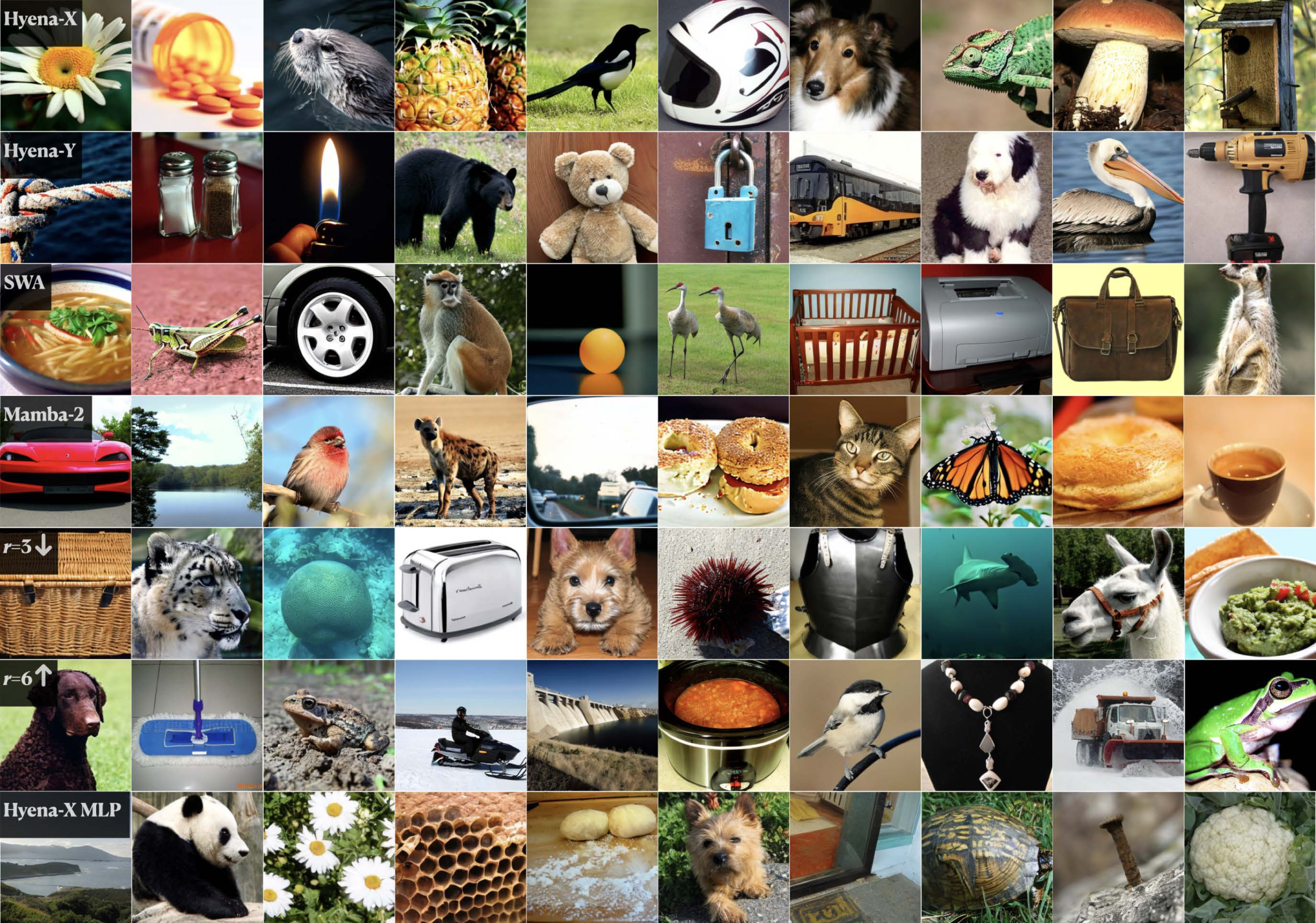
Table B.1 gives Stage 1 AdamW with β = (0.9, 0.999), no weight decay, gradient clipping at ten, 200 epochs and batch 64. It lists learning rate 10⁻³, whereas the main experiment description says 10⁻⁴. Stage 2 gives AdamW, weight decay 5×10⁻⁵, batch 256, 50K updates and 1K-step warmup to constant 10⁻⁴. The seven-row gallery includes variants from different data/settings; its best sample-associated FIDs should not be silently substituted for all Table 4 rows.
| Stage 1: Activation Distillation | |
| Initial Learning Rate | |
| Weight Decay | 0 |
| Epochs | 200 |
| Batch Size | 64 |
| Clip Norm | 10.0 |
| Optimizer | AdamW () |
| Loss Function | L1 (MHA), L2 (MLP) |
| Stage 2: Lightweight Finetuning | |
| Initial Learning Rate | |
| Weight Decay | |
| Iterations | 50,000 (100 epochs) |
| Batch Size | 256 |
| Optimizer | AdamW () |
| Scheduler | Linear Warmup over 1K steps, then constant lr |
| Training Data | 10% of ImageNet-1K (128k samples) |
B.2 Modulated Regression Targets for MHA
A modulation-aware target multiplies attention output by its learned gate. With L2 regression, this worsens FID from 2.58 to 3.00; L1 gives 2.51 in either case. This supports using ordinary, unmodulated targets with L1 for attention in this setup. The paper does not systematically vary all scales or prove that gating alone explains sensitivity.
B.3 Validation Loss Curves for Self-grafting Experiments
Validation curves use held-out 8K examples and an L2 evaluation loss regardless of the training regression objective. L1 tends to generalize better for deeper attention layers; L2 works better across the displayed MLP layers. These are isolated-operator curves and complement, rather than replace, end-to-end generation evaluation.
| Modulation-aware | IS | FID | sFID | Precision | Recall | |
| Baseline | 278.20 | 2.27 | 4.60 | 0.83 | 0.57 | |
| L2 | ✓ | 246.17 | 3.00 | 7.11 | 0.79 | 0.58 |
| ✗ | 269.31 | 2.58 | 5.75 | 0.82 | 0.58 | |
| L1 | ✓ | 272.86 | 2.51 | 5.29 | 0.82 | 0.57 |
| ✗ | 273.03 | 2.51 | 5.48 | 0.83 | 0.58 |
Appendix C Depth to Width Grafting Experiments: Additional details
Depth-to-width Stage 1 uses L1, AdamW with β = (0.9, 0.999), batch 64 and learning rate 10⁻⁴ for 200 epochs. Stage 2 uses β = (0.9, 0.95), zero weight decay, batch 256 and 230K updates, with 1K warmup then learning-rate halving every 75K steps. Its 320K examples are a quarter of ImageNet. The table’s reported aspect ratio 164.6 reflects the combined width of two branches divided by 14 stages; the caption’s 1152/14 = 82.3 example instead uses one branch width.
The authors explicitly expect speed gains to shrink at larger batch sizes because of the 712M parameter count. They also distinguish the exact rewiring used for quality from the simple fused version used for timing. No full image-generation latency curve across batch sizes is supplied.

| Stage 1: Activation Distillation | |
| Initial Learning Rate | |
| Regression Objective | L1 |
| Epochs | 200 |
| Batch Size | 64 |
| Optimizer | AdamW () |
| Stage 2: Lightweight Finetuning | |
| Learning Rate | |
| Weight Decay | 0 |
| Iterations | 230k |
| Batch Size | 256 |
| Optimizer | AdamW () |
| Scheduler | Warmup over 1K steps, half every 75k steps |
| Training Data | 25% of ImageNet-1K (320k) |
Appendix D Text-to-Image Generation Experiments: Additional details
The text-to-image supplement retains activation histograms, hyperparameters, successful outputs, prompt-alignment failures and low-quality synthetic supervision.
D.1 MHA activation plots
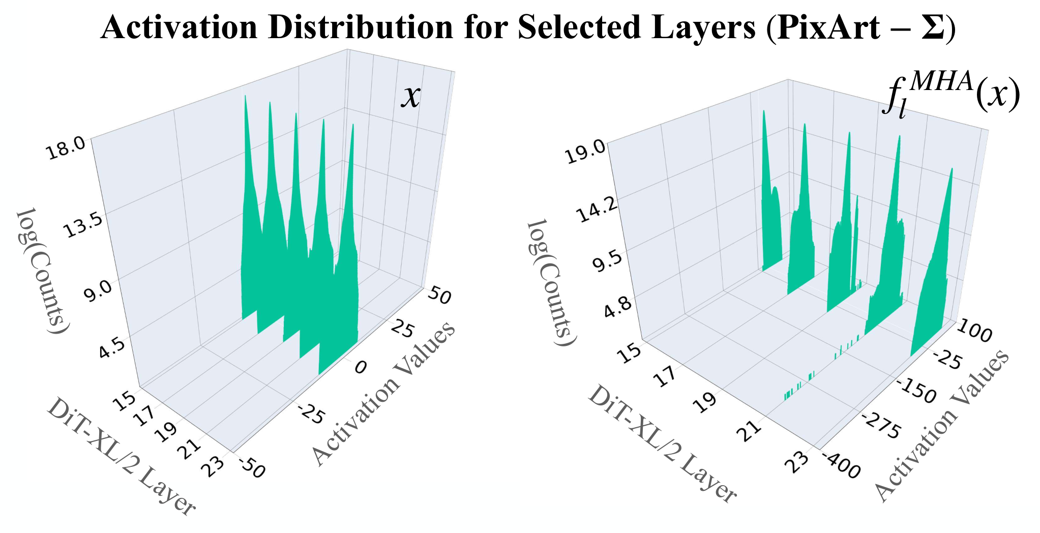
Input/output activation plots for layers 15, 17, 19, 21 and 23 show large ranges in PixArt-Σ attention. This motivates robust L1 regression but is not an independent comparison of every initialization loss on this model.
D.2 Experiment details
PixArt Stage 1 uses learning rate 10⁻⁴, weight decay 10⁻⁵, 100 epochs, batch 16 and AdamW; clipping is 0.1 for layers 20–27 and 0.01 elsewhere, with learning rate halved at epoch 50. Stage 2 uses 18K updates, effective batch 64 through accumulation, learning rate 10⁻⁵, no weight decay, 500-step warmup and rank-64 LoRA.
D.3 Generated samples and failure cases
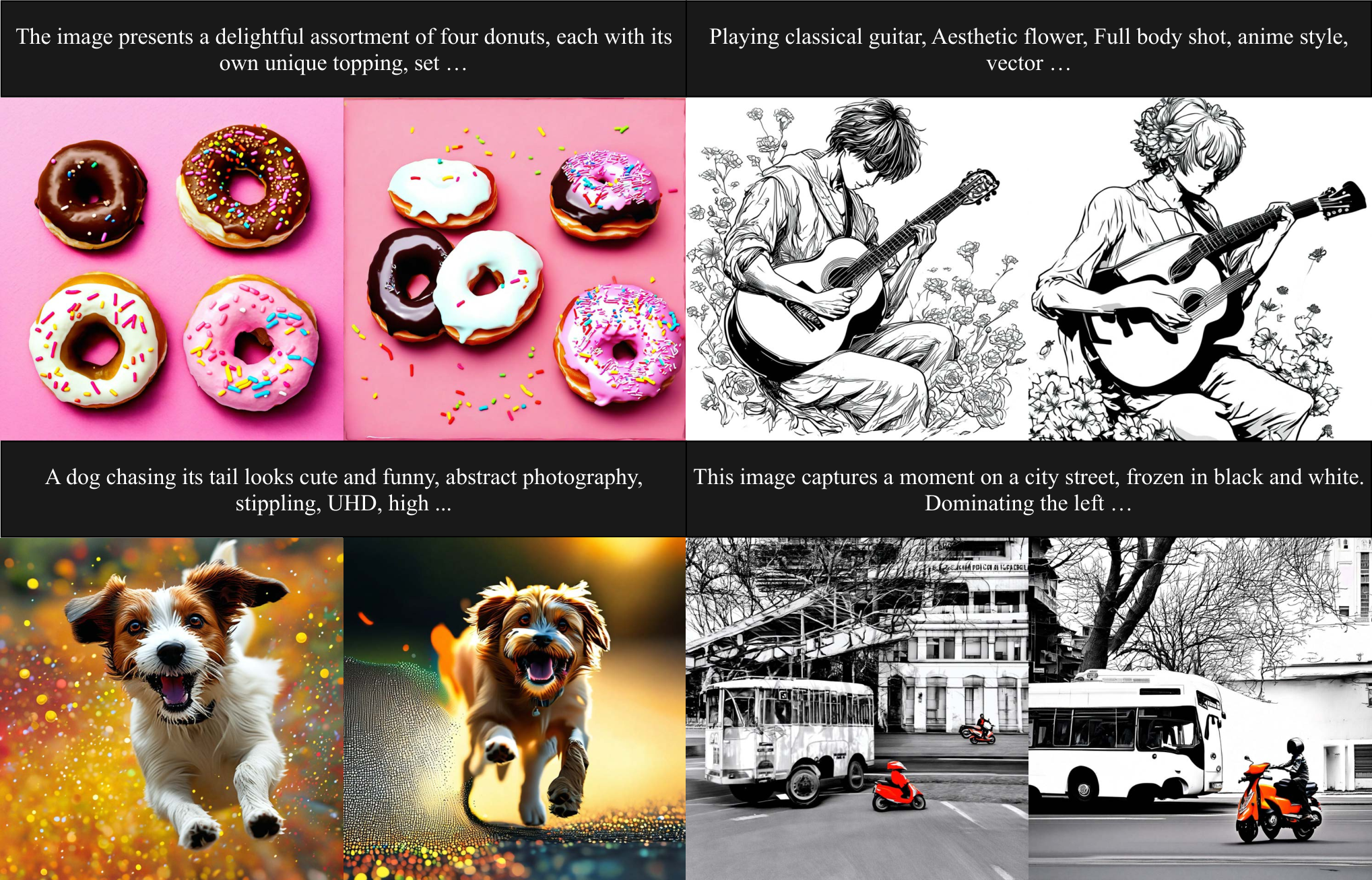
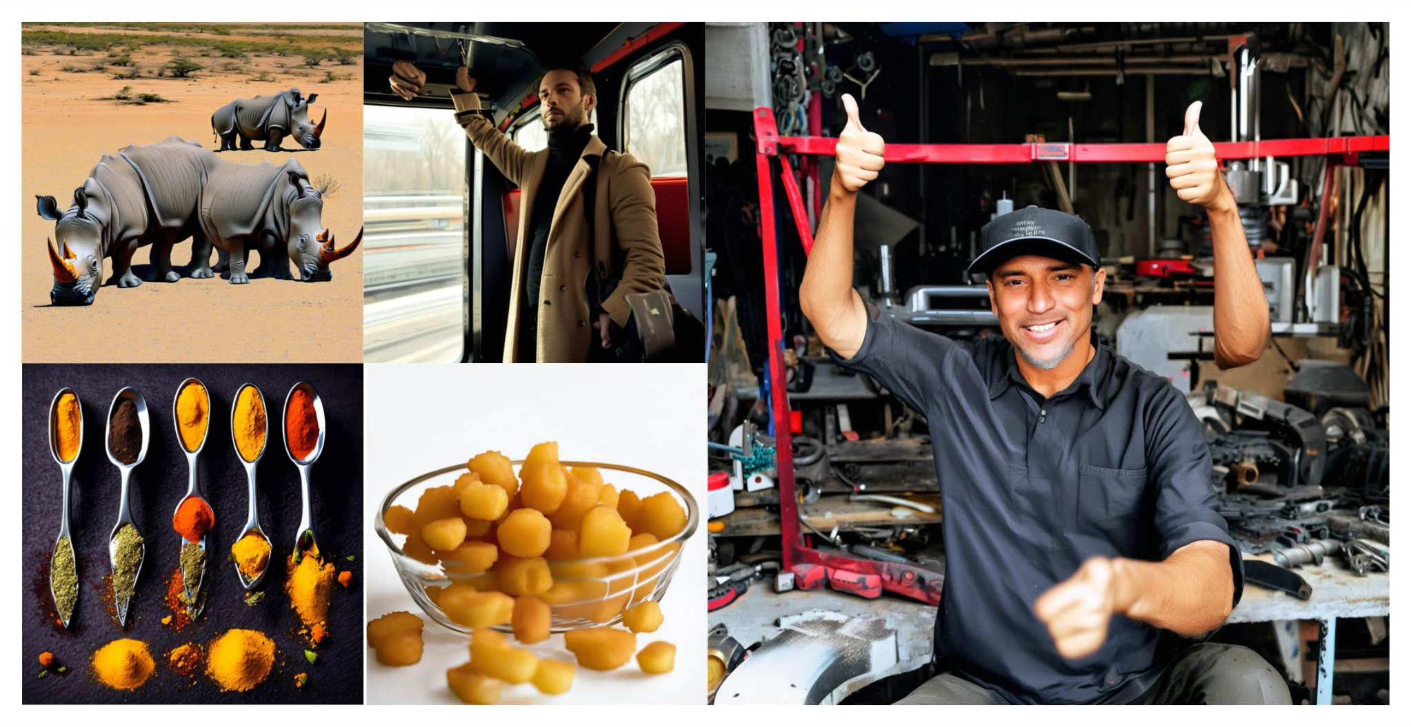
The galleries show both strengths and limits of synthetic-data adaptation. Some teacher images satisfy a prompt that the grafted model then violates, including a four-donut request and a guitar-playing character. Other prompts already receive poor teacher outputs, so both models fail. Additional examples expose implausible geometry and physics in the unfiltered training images. These figures support curation as a practical concern; they do not isolate LoRA capacity from dataset quality as the cause of every artifact.

| Stage 1: Activation Distillation | |
| Initial Learning Rate | |
| Weight Decay | |
| Epochs | 100 |
| Clip Norm Value | 0.1 (Layers 20-27), 0.01 (Other layers) |
| Batch Size | 16 |
| Optimizer | AdamW |
| Scheduler | Half lr at epochs = 50 |
| Stage 2: Lightweight Finetuning | |
| Initial Learning Rate | |
| Weight Decay | 0 |
| Iterations | 18k |
| Batch Size | 64 (with gradient accumulation) |
| Optimizer | AdamW |
| Scheduler | linear warmup (500 steps), then constant lr |
| LoRA rank | 64 |
Appendix E Hyena-X and Hyena-Y operators: Additional details
The generic Hyena equations combine dense feature projections, short convolutions and multiplicative gates with an inner convolution. Hyena-X sets the inner operator G to identity while retaining featurizer convolutions. Hyena-Y removes those three convolutions and replaces the inner long convolution with a short explicit filter. These are local operators whose overall effectiveness depends on the remaining global-attention layers and fine-tuning.
Equation
Appendix F FLOP calculation
The FLOP appendix counts dense projections, mixing, filtering, gates and output projections separately. It defines sequence length L, hidden width D, head count H, convolution width K, attention half-window w, MLP expansion r and Mamba expansion/state size. All original component formulas are retained below. FLOPs are analytical operation counts, not measured latency, and should not be equated with the speed tables.
F.1 MHA
Multi-head attention: quadratic attention mixing plus dense input/output projections.
- Input projections (Q, K, V):
- Softmax attention:
- Output projection:
F.2 SWA
Sliding-window attention: the mixing window contains 2w + 1 token positions.
- Input projections (Q, K, V):
- Sliding window attention (Bidirectional):
- Output projection:
F.3 Hyena-SE
Hyena-SE: dense projections plus three featurizer convolutions, an inner filter and gates.
- Input projections:
- Featurizer:
- Inner filter convolution:
- gates:
- Output projection:
F.4 Hyena-X
Hyena-X: retains featurizer convolutions and gates, without the inner filter.
- Input projections:
- Featurizer:
- gates:
- Output projection:
F.5 Hyena-Y
Hyena-Y: retains a short inner filter and gates, without featurizer convolutions.
- Input projections:
- Inner filter convolution:
- gates:
- Output projection:
F.6 Hyena-X (MLP)
Hyena-X as an MLP: projected channel mixing with expansion ratio r.
- Dense input projections:
- Featurizer:
- Gates:
- Dense output projections:
F.7 Mamba-2
Mamba-2: expanded projections, short convolution, featurization, state scan and output projection.
- Projections:
- Short convolution:
- Featurization:
- Associative scan:
- Output layer: