At a glance
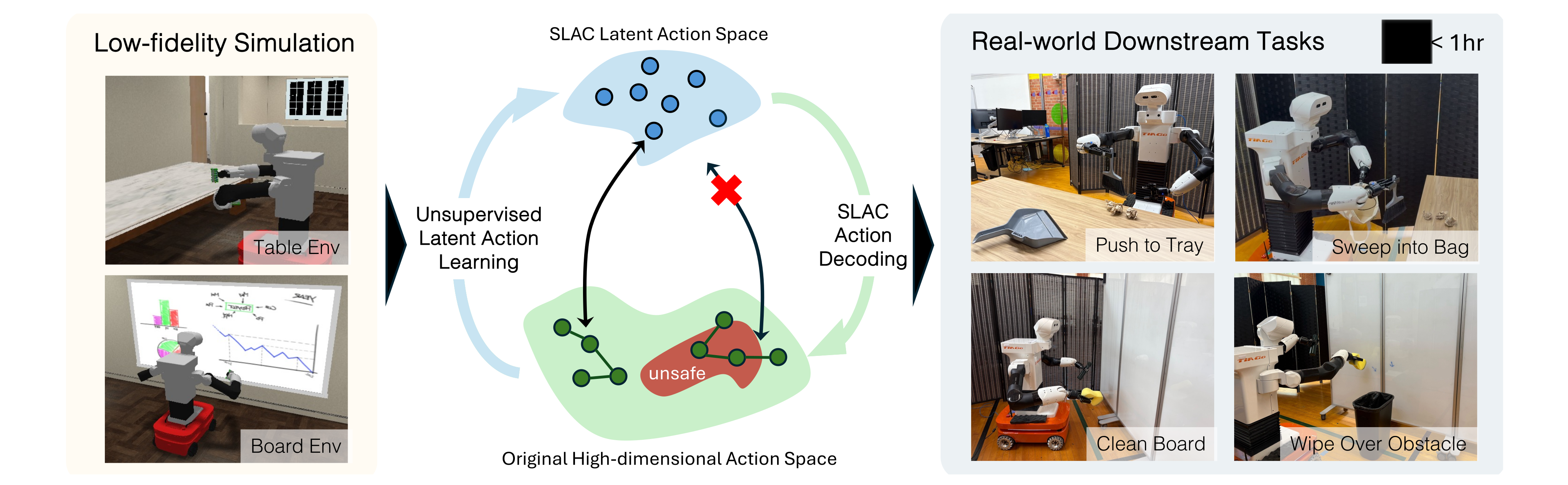
SLAC learns a reusable latent action decoder in a coarse simulator, then learns a task policy directly on the robot. Disentangled skill discovery encourages each latent factor to control a selected state factor; safety penalties discourage damaging exploration. The downstream learner combines masked value-function decomposition with frequent off-policy updates.
On a bimanual Tiago, it reaches 70–90% success over ten evaluation trials per task after 50 minutes of real-world interaction. The expanded version also tests coordinated virtual drones. Safety violations are reduced but not eliminated, and real-world interaction time excludes the simulation pretraining budget.
1 Introduction
Accurate simulation is difficult for contact, deformable objects and effects such as wiping marker traces. Direct real-world exploration avoids those modeling errors but is expensive in high-dimensional control spaces. SLAC transfers an action repertoire that reflects approximate affordances, then learns how to use that repertoire from real rewards.
The decoder supplies temporally extended, factored actions rather than a complete transferred task policy. A high-level policy can compensate for some behavior mismatch by choosing different latent actions. The approach still depends on adequate skill coverage, scene geometry, selected state factors and engineered rewards.
Novelty Statement:
This edition follows the expanded arXiv v5 manuscript dated 17 July 2026. Its CoRL 2025 predecessor was titled Simulation-Pretrained Latent Action Space for Whole-Body Real-World RL, with the same three authors.
The expansion adds multi-robot experiments, Q-decomposition during skill pretraining, and automatic inference of action–reward dependencies. These additions belong to the expanded manuscript, not necessarily to the original conference version.
2 SLAC Problem Formulation
The real task is a partially observed decision process with a composite reward. A low-fidelity simulator shares the native control interface and approximately preserves relevant affordances, while omitting detailed real dynamics, appearance and task-specific rewards.
The decoder maps a latent action and low-dimensional observations shared across simulation and reality into native controls. The task policy maps real onboard observations to latent actions. Their composition forms the deployed hierarchical policy; training the high-level policy in reality is what adapts action selection to real task outcomes.
Equations 1–2
| (1) |
| (2) |

3 SLAC Step 1: Learning Latent Action Space in Simulation
Unsupervised skill discovery pretrains the decoder without a downstream task reward. The simulator must still expose useful geometry, contacts and unsafe regions. A fixed latent action drives several low-level steps, reducing the high-level decision frequency. Algorithm 1 retains the complete pretraining loop.
3.1 Disentangled Unsupervised Skill Discovery for Structured Latent Action Space
Disentangled Unsupervised Skill Discovery (DUSDi) associates different latent factors with different state entities. A structured repertoire can be recombined more readily than an opaque one-hot skill label whose effects change many state components at once. The method builds on the authors’ earlier hierarchical-RL work.
3.1.1 DUSDi Objective
For N selected state factors, the latent action contains N categorical variables with k choices each, yielding kᴺ combinations. The objective maximizes mutual information between each latent factor and its corresponding state factor while penalizing information about all other factors.
A small penalty weight, recommended around 0.1, allows unavoidable physical coupling. The objective encourages selective effects; it cannot make inherently coupled dynamics independent or guarantee perfect disentanglement. State-factor selection is an input to the method.
Equation 3
| (3) |
3.1.2 DUSDi Tractable Optimization
Two discriminators predict each latent factor from its intended state factor and from the remaining state factors. Alternating discriminator updates with RL converts their log probabilities into an intrinsic reward. Perfect posterior estimators recover the intended mutual-information objective.
Both individual mutual-information estimates use variational lower bounds. Subtracting one bound from another does not make the combined approximate reward a guaranteed lower bound on the complete objective. Fixed target distributions can optionally focus exploration toward chosen state values; the Tiago experiments use this option.
Equations 4–6
| (4) |
| (5) |
| (6) |
3.2 Safety-Aware Latent Action Learning
The skill reward adds penalties for large actions, abrupt action changes, collisions and excessive force. The same coefficients are used across the reported environments. These are soft training preferences, not hard safety constraints or a certificate of safe execution. Algorithm 2 preserves the subsequent real-world learning procedure.
Equation 7
| (7) |
3.3 Accelerating Latent Action Space Learning through Q-Decomposition
For a fixed policy and an additive reward, linearity of expectation gives an exact decomposition of the total Q-function into one component per reward term. SLAC trains those critics separately and sums them for policy improvement; an SAC entropy bonus can be treated as another additive term.
Separating targets may ease credit assignment and reduce interference in optimization. The identity alone does not guarantee lower estimator variance or faster convergence; the empirical pretraining ablation supplies evidence for these settings.
Equation 8
| (8) |
4 SLAC Step 2: Sample-Efficient Learning of Downstream Tasks in the Real World
Factorized Latent-Action Soft Actor-Critic (FLA-SAC) trains the task policy over the frozen decoder. It combines reward-specific critics, action masks inferred from exploratory data, a high update-to-data ratio, smaller minibatches and differentiable relaxed categorical actions.
4.1 Factorized Policy Learning via Masked Q-Decomposition
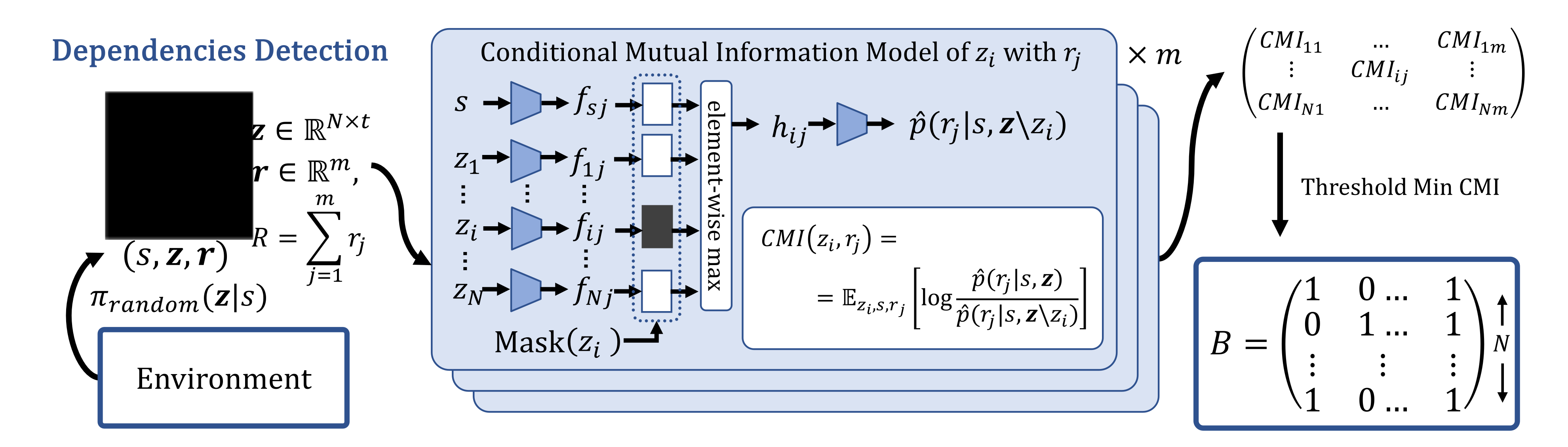
Each task reward component receives its own critic. A binary dependency matrix masks latent dimensions judged irrelevant to that component, so both value learning and actor gradients avoid unnecessary action inputs. The intended benefit is less spurious correlation and clearer credit assignment.
The source defines edges using conditional dependence of immediate reward on latent actions given state and the other actions. Applying that structure to long-horizon Q-values assumes the selected dependencies remain adequate for future return; immediate reward independence alone does not establish that in arbitrary dynamics.
Equation 9
| (9) |
4.2 Autonomous Detection of Action-Reward Dependencies
Random interactions collected for the replay-buffer warm start also train dependency models. For each reward channel, separate state/action encoders produce 128-dimensional features, combined by an elementwise maximum. Masking an action feature to −∞ lets one model predict the reward with or without that input.
The model maximizes full and partially masked reward likelihoods on training data. Held-out log-likelihood ratios estimate conditional mutual information; pairs above a threshold become dependency edges. This uses m models for m reward terms rather than one model per action–reward pair, following causal dynamics modeling. Finite exploratory coverage, model error and threshold choice can still yield incorrect masks.
Equations 10–11
| (10) | ||||
| (11) |
| Method / Task | Board | Board-Obstacle | Table-Tray | Table-Bag | ||||
|---|---|---|---|---|---|---|---|---|
| Success # | Unsafe # | Success # | Unsafe # | Success # | Unsafe # | Success # | Unsafe # | |
| SLAC (ours) | 9 / 10 | 1 | 8 / 10 | 4 | 9 / 10 | 0 | 7 / 10 | 0 |
| SERL (Luo et al., 2024) | 0 / 10 | 8 | 0 / 10 | 22 | 0 / 10 | 6 | 0 / 10 | 9 |
| Sim2Real (Tobin et al., 2017) | 2 / 10 | - | 2 / 10 | - | 4 / 10 | - | 0 / 10 | - |
| RLPD (Ball et al., 2023) | 4 / 10 | 34 | 2 / 10 | 37 | 3 / 10 | 26 | 0 / 10 | 33 |
4.3 Further Boosting Sample Efficiency via High UTD Ratio and Regularization
Ten actor–critic updates per new high-level transition reuse limited real experience. The reported setup reduces minibatch size from 256 to 64, which empirically worked better than the tested layer normalization and critic ensembles. The proposed explanation is useful gradient noise; it is not a general guarantee that smaller batches prevent overfitting.
4.4 Handling Large Discrete Action Space
Enumerating every joint categorical action becomes expensive as the factored space grows. A non-straight-through Gumbel-softmax relaxation permits gradients through sampled latent actions, with temperature fixed at 1.0. The source reports feasibility for action spaces of order one million combinations. The retained formula describes the relaxed sample, not an exact discrete gradient.
Equation 12
| (12) | ||||
5 Experimental Results
Evaluation covers four physical mobile-manipulation tasks, two simulated multi-robot tasks, and component ablations. Real-world trials, simulation curves and skill-prediction accuracy answer different questions and use different evaluation protocols.
5.1 SLAC for Real-World Mobile Manipulation
Two coarse iGibson scenes—table and whiteboard—are reported to take under 20 minutes each to construct from existing assets. The real robot uses RGB-D observations and proprioception, with a randomly initialized PointNet and MLP. A scene-specific decoder is reused across its two downstream tasks.
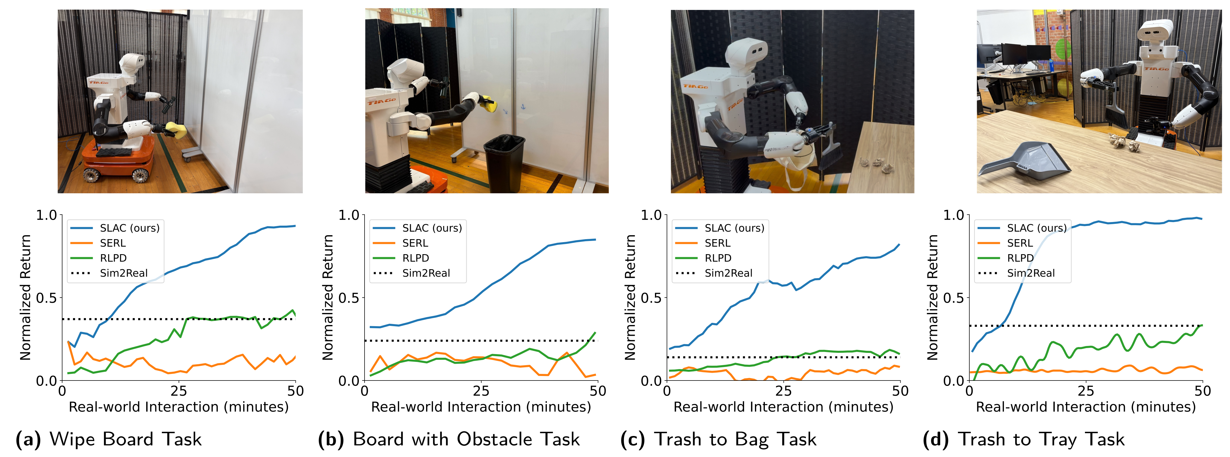
SLAC, zero-shot Sim2Real and RLPD receive 10 million simulation steps. SLAC, SERL and RLPD receive 30,000 native real-world steps, corresponding to 50 minutes of interaction. Sim2Real and RLPD additionally need task rewards and objects in simulation, so the methods require different engineering inputs.
Across Board, Board-Obstacle, Table-Tray and Table-Bag, SLAC succeeds in 9, 8, 9 and 7 of ten final trials. Training incurs 1, 4, 0 and 0 safety violations, versus SERL’s 8, 22, 6 and 9 and RLPD’s 34, 37, 26 and 33. SERL succeeds in none of the final trials; the two simulation-based baselines achieve some successes. These small evaluation samples and reported counts do not establish a universal safety guarantee.


5.2 SLAC for Multi-Robot Systems
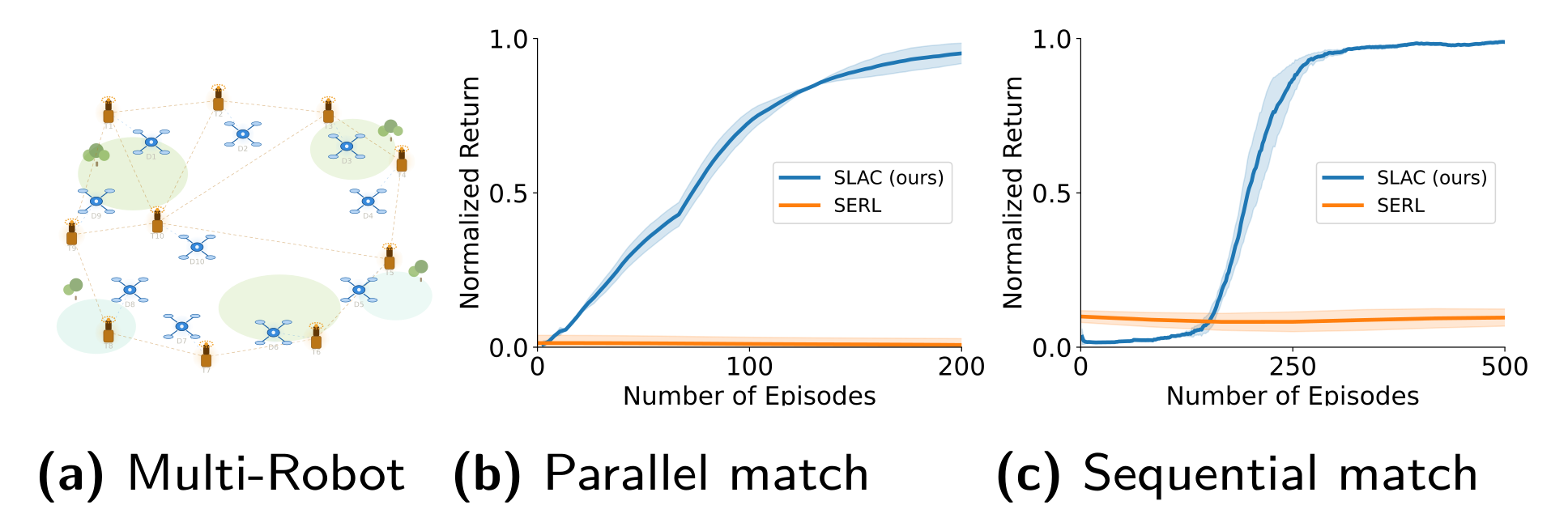
A centralized controller learns to coordinate ten virtual drones with ten matching stations. SLAC learns both simultaneous binary-command matching and ordered sequential matching, while the SERL baseline remains poor in the shown curves. Figure 7 averages three random seeds and shades the standard error.
This broadens the evidence beyond Tiago’s control structure, but the drones are simulated. It does not demonstrate transfer to a physical drone team or unrestricted embodiment independence.
5.3 Ablations
The ablations separate downstream task-learning choices from the pretraining value-function architecture. Their curves identify useful components within the tested system rather than prove each component necessary for every application.
5.3.1 Ablations of Downstream Learning
Removing disentanglement also removes the usable reward–action factorization, so that ablation changes more than one isolated mechanism. Replacing FLA-SAC with on-policy PPO or making high-level decisions at the native 10 Hz rate also reduces sample efficiency on the shown tasks. The results support structured skills, off-policy reuse and temporal abstraction as a combined design.

5.3.2 Ablations of Action Space Learning
Skill-discriminator accuracy measures how well an intended state factor reveals its latent label. Across three random seeds, decomposed critics achieve higher prediction accuracy than a monolithic critic in both virtual multi-robot and Tiago pretraining.
This indicates more distinguishable state effects under the diagnostic, not direct proof of safety or success on every downstream task. The experiment compares these architectures rather than establishing that no alternative can learn useful skills.
6 Related Work
The paper places SLAC between full-policy simulation transfer and direct physical RL, then relates it to whole-body planning, control and imitation learning.
6.1 Sim-to-Real Reinforcement Learning
Simulation-trained task policies can use cheap parallel rollouts but depend on suitable assets and dynamics. SLAC transfers a reusable action decoder and learns task selection in reality. This relaxes the need to simulate the complete task, while retaining dependence on shared control interfaces and relevant affordances.
6.2 Reinforcement Learning in the Real World
Direct real-world methods such as SERL motivate strong data reuse. High-dimensional mobile manipulation adds coordinated motion and exploration risks; earlier systems often use demonstrations or explicit behavior priors. SLAC avoids demonstrations and hand-authored motion skills, while still using designed state factors, observations and reward terms.
6.3 Whole-body Mobile Manipulation
Whole-body planners and prioritized controllers depend on models, localization and choices about competing objectives. Demonstration learning avoids some online exploration but requires suitable coordinated teleoperation data. SLAC instead trains closed-loop policies through interaction; its results do not imply that planning or demonstrations are universally inferior.
7 Conclusion
The central result is that coarse simulated affordances can support real-world RL when transferred as structured actions. A frozen decoder limits which fine-grained behaviors the task policy can express. Smaller skill vocabularies and longer execution intervals improve learning efficiency at the cost of control resolution; the best choices are task-dependent.
Decoder finetuning is proposed for finer tasks. Automated resets and reward generation remain future work, so autonomous policy updates should not be read as eliminating every human setup or reset requirement. Reported safety penalties reduce measured violations but do not eliminate them.
Support includes NSF, ONR, ARO, DARPA, Lockheed Martin and UT Austin’s Good Systems program; Jiaheng Hu also reports a Two Sigma fellowship. Peter Stone discloses compensated service as Sony AI Chief Scientist, reviewed under UT Austin’s research-objectivity policy.
Appendix A Appendix
The appendix specifies the reusable action space, continuous-action extension, safety reward, training settings and all task environments.
A.1 Policy and Training Videos
The project website provides real-world training and policy videos. The edition retains the paper’s complete still-image motion sequences in Figures 5 and 6.
A.2 Properties of the Learned Latent Action Space
The skill repertoire is task-agnostic within its training scene, but environment-aware rather than universal. The table decoder is reused for tray and bag tasks. The board repertoire tolerates the tested addition of marks and an obstacle, which were absent from its skill-training scene; broader geometric changes are not evaluated here.
A.3 Discrete vs Continuous Latent Actions
Experiments use categorical latents as a compact vocabulary of distinguishable behaviors. A proposed continuous version would give each factor a k-dimensional continuous prior and replace categorical discriminators with density estimators such as diagonal-covariance Gaussians. The mutual-information objective remains defined, but this appendix does not supply a continuous-versus-discrete experiment.
A.4 Universal Safety Reward
The universal reward penalizes squared action magnitude, squared change from the previous action, collision indicators and excessive-force indicators. Coefficients are respectively 0.01, 0.1, 0.2 and 0.05. They specify a soft penalty; physical force thresholds and a formal safety guarantee are not provided by this equation.
Equation 13
| (13) |
A.5 Hyperparameter
Each latent action executes for 50 low-level steps—five seconds at the reported 10 Hz. Decoder pretraining uses batch size 1,024, two 1,024-unit layers, 16 environments and learning rate 10⁻⁴. The table labels 4⁵ latent combinations as the latent action dimension; it is not a 1,024-coordinate vector.
Downstream learning uses batch size 64, two 256-unit layers, learning rate 4×10⁻⁴, UTD ratio 10, 60 warm-start samples and Gumbel temperature 1.0. Both complete hyperparameter tables are retained. Their single listed latent configuration does not separately enumerate every multi-robot setting.
| Name | Value | |
|---|---|---|
| SAC | optimizer | Adam |
| activation functions | ReLU | |
| learning rate | ||
| batch size | 1024 | |
| critic target | 0.01 | |
| MLP size | [1024, 1024] | |
| n updates | 2 | |
| # of environments | 16 | |
| entropy coefficient | 0.0 | |
| log std bounds | [-10, 2] | |
| warmup samples | 24000 | |
| latent action dimension |
A.6 Mobile Manipulation Environment Description
Tiago’s 17 native controls comprise three base velocities, two head joints and two six-dimensional end-effector pose increments. The task policy receives a segmented 320×240 RGB-D observation reduced to 50 points plus seven proprioceptive values. Reward is delivered at the end of each high-level step.
A.6.1 Board Environment
The board decoder observes proprioception, previous actions, board-relative distance/orientation and contact history. RANSAC estimates board geometry in reality. Skill factors cover contact history, base position, camera view and contact force.
Clean Whiteboard rewards looking at, approaching and removing the target mark while penalizing collisions or excessive force. Wipe Board over Obstacles adds an intervening obstacle with the same reward formulation. The stated success criterion requires all four conditions, not just visible wiping.
A.6.2 Table Environment
The table decoder uses proprioception, previous actions and RANSAC-estimated table-relative geometry. Its factors cover both end-effectors, base location and camera view; table collision is penalized.
Push to Tray rewards looking at and approaching the garbage, pushing it into the tray and avoiding dangerous contact. Sweep to Bag starts with a bag already in the left gripper; it rewards pushing garbage off the table while keeping the bag nearby. This setup does not learn bag pickup or specify an explicit garbage-in-bag reward term.
A.7 Multi-Robot Environment Description
The simulated multi-robot system has ten drones and ten uniquely matching stations, a 70-dimensional observation and 50-dimensional action space. Five controls per robot govern acceleration and interaction.
Parallel Match requires simultaneous compliance with binary interaction indicators. Sequential Match requires visiting matching stations in a prescribed episode-level order. Incorrect interactions are penalized; both tasks use a centralized controller.