Overview
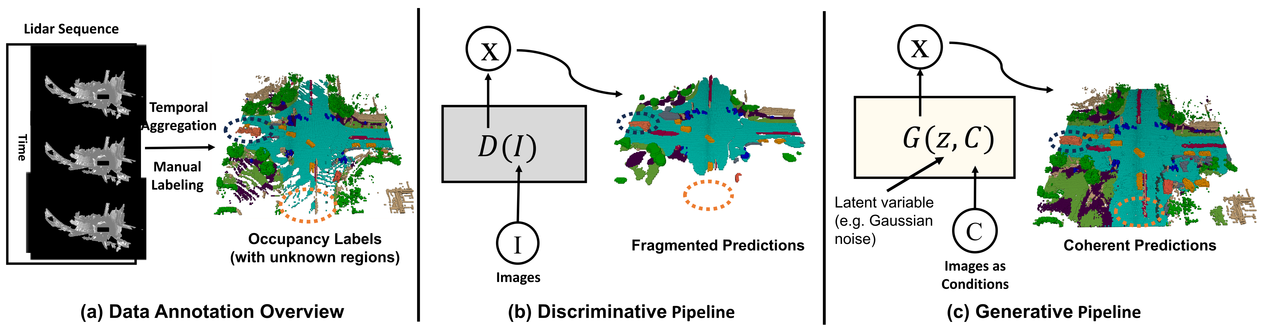
Figure 1 contrasts incomplete LiDAR-derived annotations, a direct prediction pipeline and conditional generative prediction. The edition retains the complete seven-page source, including every figure, table and equation; this version contains no separate supplementary appendix.
At a glance
DiffOcc predicts a distribution of semantic 3D occupancy grids conditioned on multi-camera features. A BEV encoder lifts images into spatial features, and a diffusion denoiser uses those features to reconstruct voxel labels. The study compares representations, conditioning signals and guidance methods.
On Occ3D-nuScenes, discrete diffusion improves aggregate occupancy accuracy and several offline planning measures. Results are particularly strong in camera-invisible and low-visibility regions, where the learned prior can fill gaps in incomplete observations. These experiments do not establish safety or freedom from hallucination.
I INTRODUCTION
Multi-view images leave some voxels unobserved, and aggregated LiDAR annotations can themselves be sparse or noisy. Directly predicting each scene from images may produce fragmented geometry. DiffOcc instead models plausible occupancy structure and samples it under visual conditioning.
The proposed advantages are spatial consistency, completion of unseen regions, multiple plausible outputs and an adjustable sampling budget. These motivate the design study. The evaluation uses 0.4 m voxels, so the introduction’s general reference to centimeter-level precision is not the tested grid resolution.
II Formulation
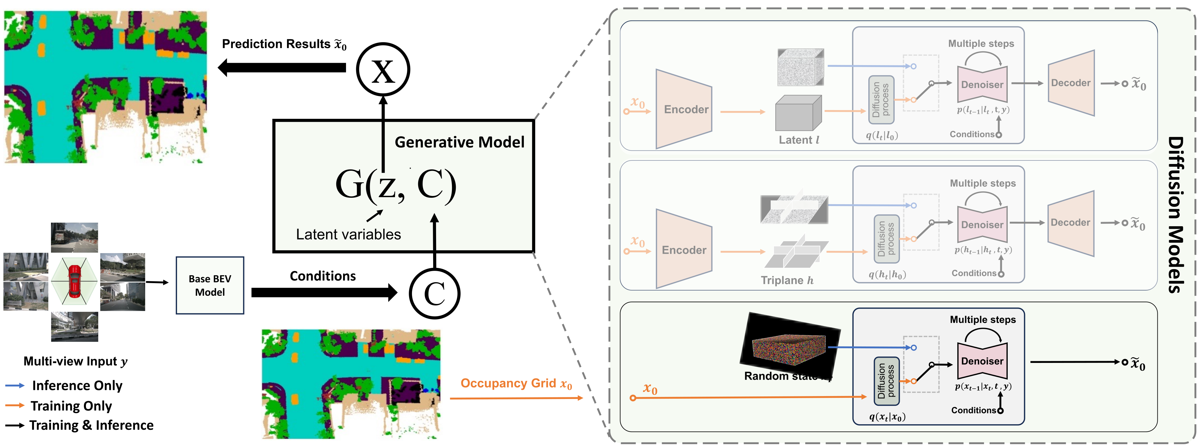
The framework adapts continuous and categorical diffusion models to semantic occupancy. Forward corruption defines a training target; a learned reverse process reconstructs the scene while conditioning on encoded images.
II-A Diffusion Models
Continuous diffusion adds Gaussian noise with a time-dependent variance and learns a Gaussian reverse transition. Discrete diffusion instead applies a categorical transition matrix to semantic labels and predicts reverse class probabilities. The retained equations state both versions without changing the source notation.
Equations 1–4
| (1) |
| (2) |
| (3) |
| (4) |
II-B Training Diffusion Models
The forward posterior is available from the corruption process and the clean sample. Training minimizes KL divergence between that posterior and the learned reverse transition. The implemented denoiser predicts the clean label configuration x₀, rather than directly outputting the preceding noisy state.
Equations 5–6
| (5) |
| (6) |
II-C Occupancy Prediction as Conditional Generation
The generated variable becomes the 3D occupancy grid, and multi-view visual features condition each reverse step. A base BEV model computes those features once; the denoiser repeatedly reuses them. Both continuous latent variables and discrete semantic labels fit this conditional formulation.
Equations 7–8
| (7) |
| (8) |
III Key Design Decisions
The design study varies the denoiser, visual encoder, occupancy representation, guidance strategy and conditioning signal. The final system uses discrete labels, classifier-free guidance and features taken before the encoder’s final classifier.
III-A Denoiser Network Architecture
A cylindrical point-cloud segmentation network is adapted as a U-Net-like denoiser. Sinusoidal diffusion-time embeddings pass through two linear layers with SiLU activation. A learned input embedding converts corrupted categorical labels into continuous features before clean-label prediction.
III-B Visual Encoder
BEVFormer lifts camera images into spatial features to constrain generation. The expensive visual encoder runs once per scene, rather than once per denoising step. Later experiments also use PanoOcc features, demonstrating compatibility with a second encoder.
III-C Options for Diffusion Modeling across Representations
Spatial-latent diffusion encodes voxels with a 3D convolutional autoencoder and decodes semantic probabilities with an implicit MLP. Triplane diffusion pools the same latent into three orthogonal planes and sums bilinearly interpolated features at each 3D query. Discrete diffusion directly corrupts voxel categories with uniform transitions.
Table I reports mIoU 30.65 for spatial latents, 30.23 for triplanes and 31.78 for discrete labels, versus 23.67 for its BEVFormer reference. The authors choose discrete labels, hypothesizing that they avoid autoencoder information loss. This is a plausible explanation, not an isolated measurement of that loss.
III-D Guidance techniques
Classifier-free guidance combines conditional and unconditional logits using the source convention ℓ = (s+1)ℓc − sℓu. Classifier guidance instead follows gradients from a discriminative occupancy classifier. CFG is better at every tested scale in Table II, reaching 32.45 mIoU at scale 3.5 versus CG’s 29.97.
The authors attribute CG’s weakness to classifier errors, but do not separately isolate that cause. Scale 3.5 is used in later experiments; under this formula, zero would give the unamplified conditional logits.
Equation
III-E Condition Options
Conditioning can use predicted labels (C-PR), final logits (C-L), or features before the classifier (C-R). Table III gives 32.45, 31.77 and 40.63 mIoU respectively. C-R also permits joint encoder/denoiser training, so the comparison changes both information content and trainability.
The best conditioning choice is adopted for the main experiments. Absolute ablation scores and the later benchmark scores differ; the source does not fully itemize every setting behind those differences.
Method
Backbone
Image size
mIoU
Others
Barrier
Bicycle
Bus
Car
Cons. Veh
Motorcycle
Pedestrian
Traffic cone
Trailer
Truck
Driv. Sur
Other flat
Sidewalk
Terrain
Manmade
Vegetation
MonoScene [16]
R101
9001600
6.0
1.7
7.2
4.2
4.9
9.3
5.6
3.9
3.0
5.9
4.4
7.1
14.9
6.3
7.9
7.4
1.0
7.6
BEVFormer [11]
R101
9001600
22.36
2.7
35.57
8.43
32.09
40.19
12.15
14.99
17.04
16.18
16.49
27.88
48.75
27.64
28.87
25.15
11.16
14.84
RenderOcc [17]
SwinB
5121408
24.46
4.74
26.64
12.48
23.13
22.25
13.29
10.97
13.92
13.18
23.28
21.21
67.62
33.02
43.37
44.18
19.11
23.42
FB-Occ [15]
R101
256704
38.33
8.52
43.85
26.25
42.79
49.59
22.94
27.65
27.73
26.98
34.41
36.73
78.36
41.41
47.01
49.80
44.89
42.54
BEVDet [18]
SwinB
5121408
39.08
7.17
46.11
22.09
46.2
51.57
24.08
25.15
27.11
25.1
34.77
37.89
78.92
42.13
50.63
50.54
49.04
45.91
PanoOcc [19]
R101
8641600
42.32
8.37
49.86
28.11
51.45
58.97
24.82
34.6
32.29
30.15
37.75
46.77
80.8
42.97
51.25
45.38
44.33
42.32
BEVFormer [11]
R101
9001600
35.62
4.96
41.48
15.81
44.65
50.97
20.9
20.74
25.87
22.32
33.11
35.59
78.05
39.04
44.49
48.17
41.08
38.25
PanoOcc [19]
R101
8641600
42.15
8.51
49.22
28.35
50.37
58.48
25.58
34.3
31.16
30.49
38.38
45.37
81.2
44.07
50.8
51.63
44.83
42.15
DiffOcc (BEVFormer)
R101
9001600
42.67
8.59
47.61
26.02
54.21
58.11
26.2
29.55
31.1
29.61
38.93
46.19
81.23
44.01
50.99
51.6
51.93
49.56
DiffOcc (PanoOcc)
R101
8641600
43.08
7.86
48.67
25.66
55.73
57.14
27.17
32.33
30.06
30.1
40.42
48.48
82.01
43.98
52.06
52.03
49.98
48.69
IV Fascinating Properties of Diffusion Models for Occupancy Prediction
The paper interprets diffusion’s learned distribution as a scene prior and explores completion, noisy regions, diverse samples and inference-step control. These are empirical behaviors under the chosen dataset and setup, rather than properties guaranteed for every diffusion model.
IV-A 3D Scene Prior
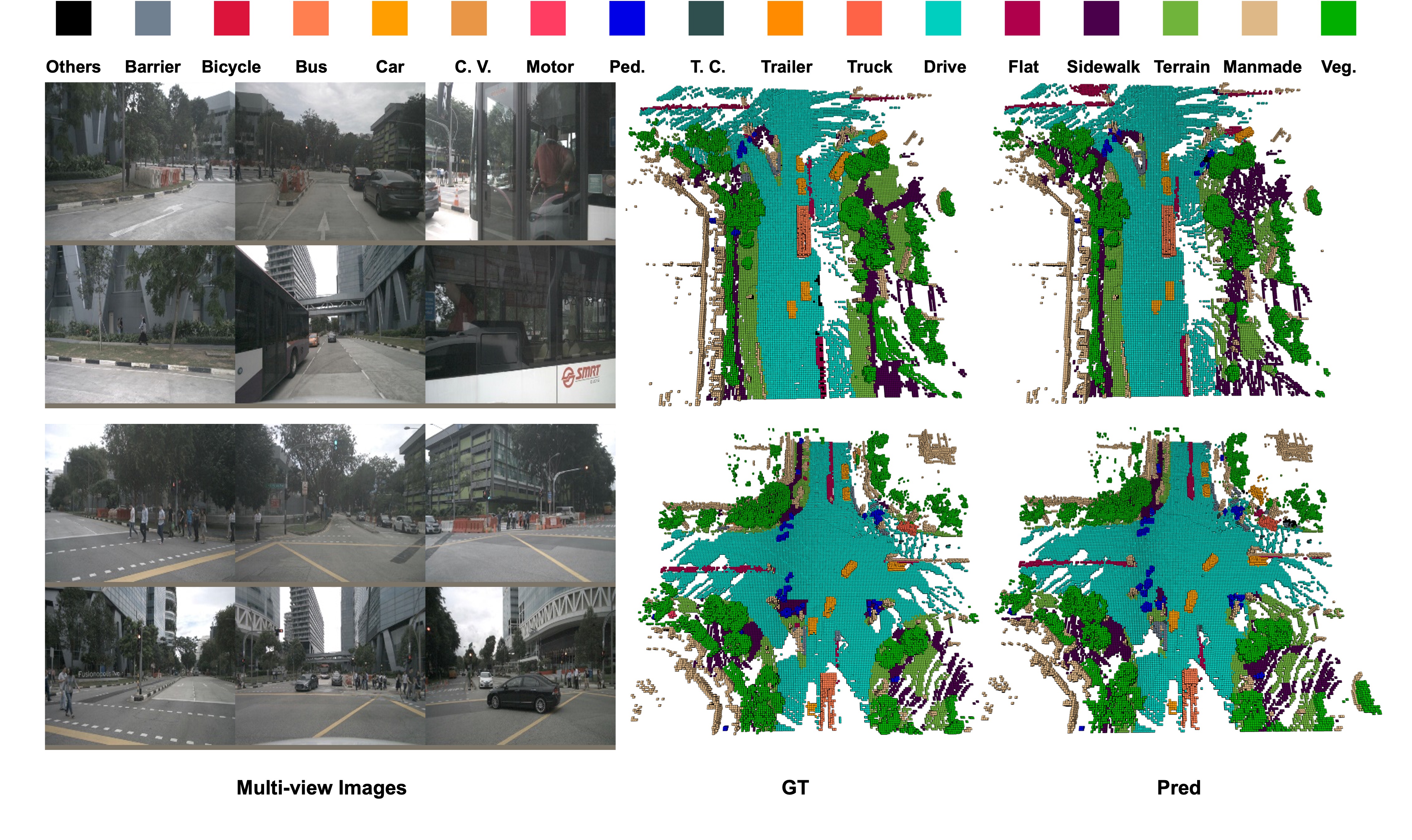
Joint modeling can favor coherent geometry and semantic relationships among voxels. Figures 3 and 5 show more complete-looking predictions, including regions with weak image evidence. Such plausible completion is useful but can also introduce unseen structure that annotations cannot verify.

IV-B Robustness to Noisy Data
The forward corruption process supplies augmentation, which may reduce sensitivity to imperfect occupancy labels. The reported evidence compares distant and rarely visible regions; it does not inject controlled label noise or estimate a noise-response curve. Those regions mix noise with occlusion, distance and distributional difficulty.
IV-C Multi-Modal Occupancy Distributions
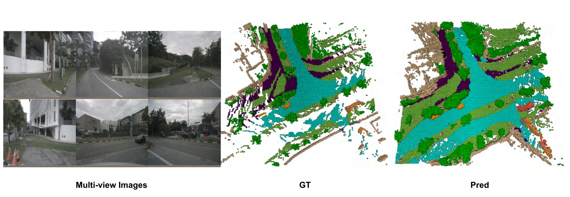
Different 3D scenes can explain the same images. Repeated conditional diffusion samples can represent some of that ambiguity, as illustrated in Figure 4. The paper does not report calibrated uncertainty, quantitative diversity/coverage metrics, or planning that explicitly reasons over multiple samples.
IV-D Dynamic Inference Steps
The number of reverse steps provides an inference-cost control. Accuracy need not increase monotonically with more steps, because the trained reverse process and its sampled inputs can differ from the ideal corruption distribution.
V Evaluation
Evaluation combines semantic occupancy IoU, subsets defined by observability or distance, a sampling-step ablation and an offline planning comparison. Different baselines use different image sizes and backbone/pretraining settings, retained in the tables.
V-A Experimental Setup
Occ3D-nuScenes covers x/y from −40 to 40 m and z from −1 to 5.4 m using 0.4 m voxels and 17 semantic categories. The collection vehicle has six cameras, LiDAR and five radars; the proposed predictor is conditioned on camera-derived BEV features, not all sensors.
The source uses a 1,000-step training diffusion process and normally ten inference steps with CFG scale 3.5. Other training settings are said to follow established occupancy methods but are not fully enumerated here. Table IV evaluates with a LiDAR mask.
V-B Comparison with State-of-the-art Methods
With the reimplemented BEVFormer encoder, DiffOcc increases mIoU from 35.62 to 42.67, a 7.05-point gain. With the non-segmentation-pretrained PanoOcc row, it increases from 42.15 to 43.08, a 0.93-point gain; the prose reports 0.97, which does not match the displayed values.
The gains are aggregate, not uniform across classes: DiffOcc with PanoOcc lowers several class IoUs while improving others. The original and reimplemented BEVFormer rows differ substantially, so the appropriate paired reference is important.
| Method | Backbone | mIoU |
|---|---|---|
| BEVFormer | R101 | 26.03 |
| PanoOcc | R101 | 30.13 |
| DiffOcc (BEVFormer) | R101 | 30.73 |
| DiffOcc (PanoOcc) | R101 | 32.04 |
| Method | 5% | 10% | 20% | 50% |
|---|---|---|---|---|
| BEVFormer | 28.1 | 29.55 | 32.26 | 33.59 |
| DiffOcc (BEVFormer) | 33.82 | 36.02 | 39.69 | 41.64 |
| Method | L2 (m) | Collision (%) | ||||||
|---|---|---|---|---|---|---|---|---|
| 1s | 2s | 3s | Avg. | 1s | 2s | 3s | Avg. | |
| G.T. Occ. | 1.62 | 3.02 | 4.20 | 2.95 | 2.97 | 3.77 | 4.53 | 3.76 |
| BEVFormer | 1.82 | 3.39 | 4.73 | 3.31 | 2.52 | 3.26 | 4.72 | 3.50 |
| DiffOcc (BEVFormer) | 1.66 | 3.08 | 4.29 | 3.01 | 2.39 | 3.26 | 4.37 | 3.34 |
| BEVFormer† | 2.46 | 5.27 | 7.71 | 5.15 | 1.66 | 4.29 | 8.22 | 4.72 |
| DiffOcc (BEVFormer)† | 1.56 | 2.91 | 4.12 | 2.87 | 1.86 | 2.74 | 4.87 | 3.16 |
V-C Reasoning with Prior in Camera-Invisible Regions
Using the dataset’s camera-invisibility labels, DiffOcc reaches 36.45 mIoU with BEVFormer versus 21.42 for the reimplementation, and 36.83 with PanoOcc versus 30.13. These gains support stronger completion in the annotated invisible subset.
Aggregated LiDAR does not label every unobserved region, so the metric cannot validate all generated geometry. Denser qualitative predictions can exceed annotation coverage without proving that every added surface is correct.
V-D Performance In Noisy Regions
In distant regions around or beyond 20 m, Table VI reports 30.73 versus 26.03 mIoU for the BEVFormer pair and 32.04 versus 30.13 for PanoOcc. For voxels with training-set visibility probability below 5%, DiffOcc improves 28.10 to 33.82, with gains also at 10%, 20% and 50% thresholds.
These subset comparisons demonstrate stronger performance where observations are difficult. They support robustness to those conditions, but do not by themselves establish learning of a noise-free underlying distribution.
V-E Inference Steps.
Table IX gives 40.48 mIoU at one step, 40.63 at two, 42.12 at ten, a peak of 42.14 at 15, and 40.47 at 50. The paper reports poorer results when following the full training-length chain and instead uses early clean-sample reconstructions.
The source proposes train/test distribution mismatch as an explanation. It provides step counts, not measured wall-clock latency or compute-normalized comparisons, so deployment speed cannot be inferred directly.
V-F planning
A simplified UniAD-based planning module is trained with occupancy annotations in place of BEV features, then evaluated with different occupancy inputs. Under the standard mask setting, DiffOcc lowers average trajectory L2 error from 3.31 to 3.01 m and collision rate from 3.50% to 3.34%.
Without visibility masks in training/evaluation, the BEVFormer pair changes from 5.15 to 2.87 m and 4.72% to 3.16%. These averages improve, although the one-second collision rate rises from 1.66% to 1.86%. The ground-truth-occupancy row gives 2.95 m and 3.76%, so the unmasked generative row scores better in this offline setup.
Incomplete annotations and the planner’s input distribution complicate treating ground truth as an upper bound. This experiment does not establish closed-loop driving safety or absence of harmful hallucinations.
VI Related Works
DiffOcc connects semantic scene completion and occupancy prediction with generative perception. Its design study emphasizes distributions and conditioning choices alongside final segmentation accuracy.
VI-A 3D Occupancy Prediction and Completion
Semantic scene completion reconstructs dense geometry and semantics from partial observations. Occupancy prediction similarly estimates a labeled 3D volume, often emphasizing dynamic and static objects within sensor coverage. The learned prior can support completion, although the main evaluation remains Occ3D occupancy prediction.
VI-B Generative Models for Autonomous Driving and Robotics
MapPrior combines discriminative BEV perception with a generative layout prior; UltraLiDAR uses vector-quantized autoencoding; Copilot4D applies discrete diffusion to LiDAR sequences. DiffBEV and OccGen also use diffusion-related methods. This work studies occupancy representations, guidance, conditioning and several downstream behaviors rather than establishing that diffusion is unique to this task.
VII Conclusion & Discussion
Conditional discrete diffusion improves occupancy and offline planning metrics in the reported setup, especially under limited visibility. The best design uses pretrained spatial features, joint feature conditioning and modest sampling budgets.
Latency remains a concern; few-step inference is promising but lacks timing measurements here. Higher mean IoU and better average planning scores do not prove that hallucinations are harmless. Broader datasets, calibrated multi-sample uncertainty, controlled noise tests, complete implementation settings and closed-loop evaluation remain unresolved.
ACKNOWLEDGMENT
The work is supported by China’s National Key R&D Program (2022ZD0161700) and the Tsinghua University Initiative Scientific Research Program.