Overview
Challenger generates adversarial traffic trajectories and renders them into six-camera driving videos for testing vision-based planners.
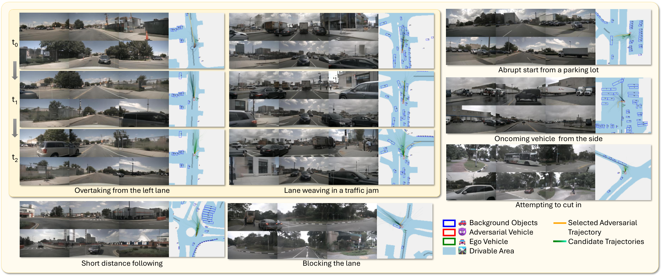
At a glance
Challenger combines a trajectory diffusion model, kinematic simulation, a geometric challenge score, and multiview video generation. It searches over traffic motion before paying the cost of rendering, then tests four pretrained autonomous-driving planners on the resulting Adv-nuSc dataset. Predicted collisions rise substantially, and failure-selected scenarios often affect multiple architectures. The evidence concerns open-loop three-second plans; it does not measure closed-loop driving or physical crash rates.
1 Introduction
Naturalistic driving datasets contain relatively few deliberately difficult traffic interactions. Adversarial trajectory generators and photorealistic video generators address different parts of this testing problem. Challenger joins them: it changes a background vehicle’s motion within a recorded scene, rejects physically unsuitable or already-colliding trajectories, and synthesizes camera observations for the remaining interaction. Its contribution is an automated sensor-level stress-test generator, not a deployed driving policy or a certified safety assessment.
2 Related Work
Prior work provides adversarial traffic generation, controllable driving imagery, and end-to-end planning architectures; Challenger integrates these capabilities in an offline testing pipeline.
2.1 Driving Trajectory for Planning
Naturalistic adversarial testing, rare-event simulation, diffusion planning, and language-conditioned traffic generation improve coverage of unusual behaviors. Challenger draws its resample-and-denoise search from Diffusion-ES [14], adding kinematic feasibility checks and a renderer-compatible geometric score. Unlike optimization against every rendered candidate, this search can proceed without querying a victim driving model.
2.2 Driving Video Generation
Driving video generators condition on scene structure to maintain geometry, motion, and camera consistency. Challenger uses MagicDriveDiT [24] as its renderer, while supplying traffic motions selected to challenge the ego vehicle. The rendering model is an existing component; the proposed contribution is the adversarial scenario-generation process around it.
2.3 End-to-End Autonomous Driving
End-to-end driving systems combine perception and planning, but their learned predictions may fail under unusual interactions. The paper evaluates official pretrained UniAD, VAD, SparseDrive, and DiffusionDrive models. Diverse architectures provide a useful transfer test, although sharing failures on this generated distribution does not establish a common internal cause.
3 Method
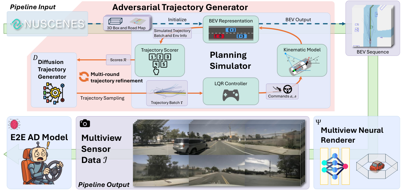
The pipeline samples trajectories, simulates their execution, scores geometric plausibility and proximity, repeatedly refines promising candidates, and renders only selected scenes.
3.1 Diffusion Trajectory Generator
An unconditional diffusion model is trained on nuPlan trajectories [66], represented by fixed-length sequences of two-dimensional waypoints in local coordinates. It can draw new motion plans from noise or perturb an existing plan by partial noising and denoising. The learned prior supplies motion diversity; because it is unconditional, environmental compatibility must be established downstream.
3.2 Physics-aware Planning Simulator
A linear-quadratic regulator tracks each candidate using steering and acceleration commands, while a kinematic bicycle model produces the resulting vehicle motion and bounding boxes. This checks a simplified execution model rather than treating sampled waypoints as automatically feasible. It does not model realistic crash dynamics, which is one reason the generator rejects collisions.
3.3 Trajectory Scorer
The score penalizes leaving drivable space and contact with other vehicles, including the recorded ego vehicle, while favoring close approaches. It operates on simulated trajectories and bounding boxes, avoiding expensive rendering and planner evaluation for every candidate. Proximity is a surrogate for difficulty, not a direct guarantee that any given driving model will fail.
3.4 Multi-round Trajectory Refinement
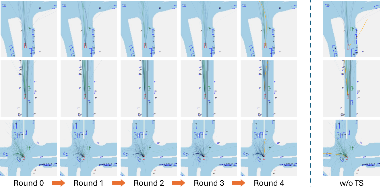
Each round simulates and scores a batch, resamples promising candidates with replacement, then partially noises and denoises them to explore nearby motions. The trained generator stays fixed during this search. The final scene is retained only if the adversarial vehicle avoids collisions and the original ego trajectory remains collision-free.
This establishes feasibility of the recorded reference path under the generator’s checks, not recoverability by every learned planner from synthetic observations. The paper’s main prose and algorithm select the highest score, whereas the appendix defines lower scores as better and samples with a negative-score softmax. The original algorithm is retained, including its use of the pre-resampling trajectory symbol in the noising line; these notation inconsistencies should be resolved before implementation.
3.5 Multiview Neural Renderer
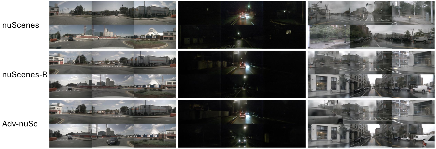
MagicDriveDiT receives the modified three-dimensional boxes and bird’s-eye-view map and generates synchronized observations for six cameras. Rendering occurs after trajectory search and filtering. Re-rendering unchanged validation scenes provides a useful control for image-generation shift, though the adversarial motions can introduce a different shift from unchanged scenes.
4 Experiments
The experiments compare open-loop planning collisions, transfer across architectures, component ablations, visual quality, and generation cost.
4.1 Experiment Setup
The base nuScenes validation split contains 150 twenty-second scenes and 6,019 annotated samples. Its unchanged scenes are re-rendered as nuScenes-val-R. Challenger produces 156 adversarial scenes and 6,115 samples for Adv-nuSc. Four official pretrained vision-based models predict three-second ego trajectories from multiview images; the test evaluates these predictions against scene geometry rather than rolling the policies through an interactive closed loop.
4.2 Results on the Adv-nuSc Dataset
At three seconds, collisions rise from 0.61% to 6.96% for UniAD, 0.42% to 9.08% for VAD, 0.238% to 2.430% for SparseDrive, and 0.169% to 3.646% for DiffusionDrive. The corresponding unchanged re-rendered rates are 0.64%, 0.59%, 0.370%, and 0.403%. Thus rendering alone alters performance, but the adversarial scenarios cause much larger absolute increases.
The table’s average columns average one-, two-, and three-second rates; they are different from the three-second endpoint metric. Its annotated multiplicative increases do not uniformly match simple ratios of the displayed averages, so the direct rates are the clearest quantitative evidence. No closed-loop collision probability is established.
| Dataset | AD Model | 1s | 2s | 3s | avg | AD Model | 1s | 2s | 3s | avg | ||
|---|---|---|---|---|---|---|---|---|---|---|---|---|
| nuScenes-val | UniAD [8] | 0.10% | 0.15% | 0.61% | 0.29% | SparseDrive [10] | 0.020% | 0.063% | 0.238% | 0.107% | ||
| nuScenes-val-R | 0.07% | 0.24% | 0.64% | 0.32% | 0.010% | 0.090% | 0.370% | 0.156% | ||||
| Adv-nuSc | 0.80% | 4.10% | 6.96% | 3.95% | 0.029% | 0.618% | 2.430% | 1.026% | ||||
| nuScenes-val | VAD [9] | 0.11% | 0.24% | 0.42% | 0.26% | DiffusionDrive [11] | 0.059% | 0.068% | 0.169% | 0.099% | ||
| nuScenes-val-R | 0.19% | 0.32% | 0.59% | 0.37% | 0.030% | 0.055% | 0.403% | 0.163% | ||||
| Adv-nuSc | 4.46% | 7.59% | 9.08% | 7.05% | 0.068% | 1.299% | 3.646% | 1.671% |
4.3 Qualitative Examples of Adversarial Driving Scenarios
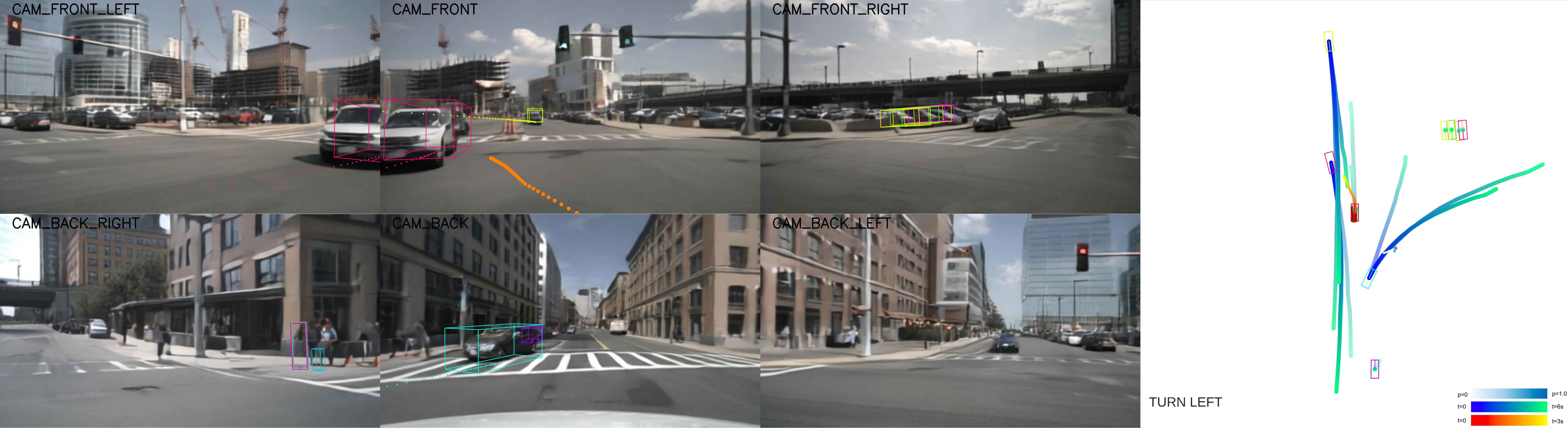
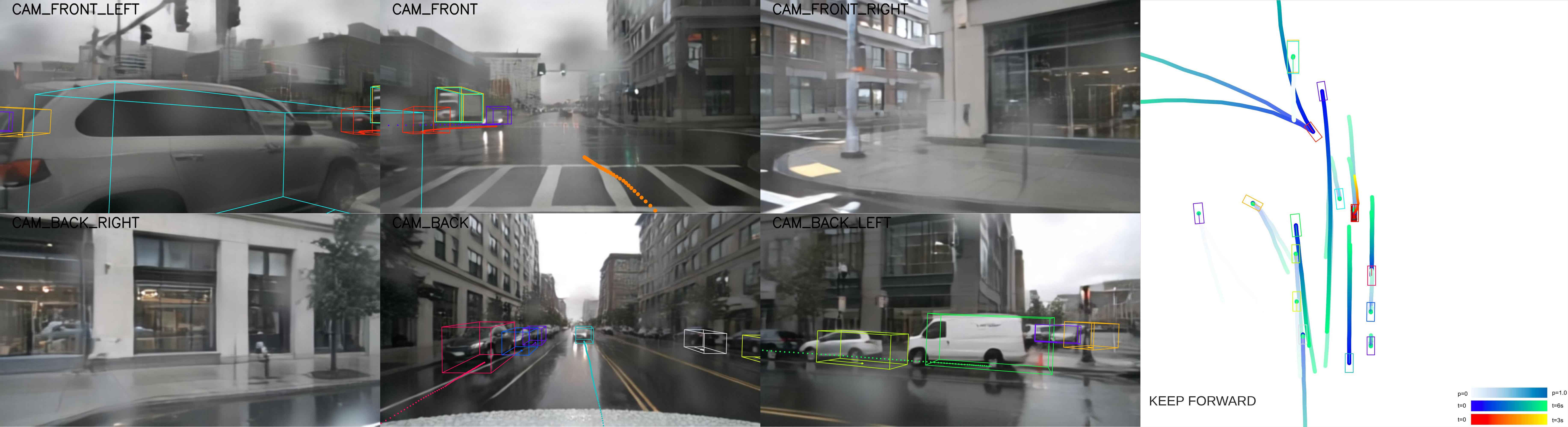
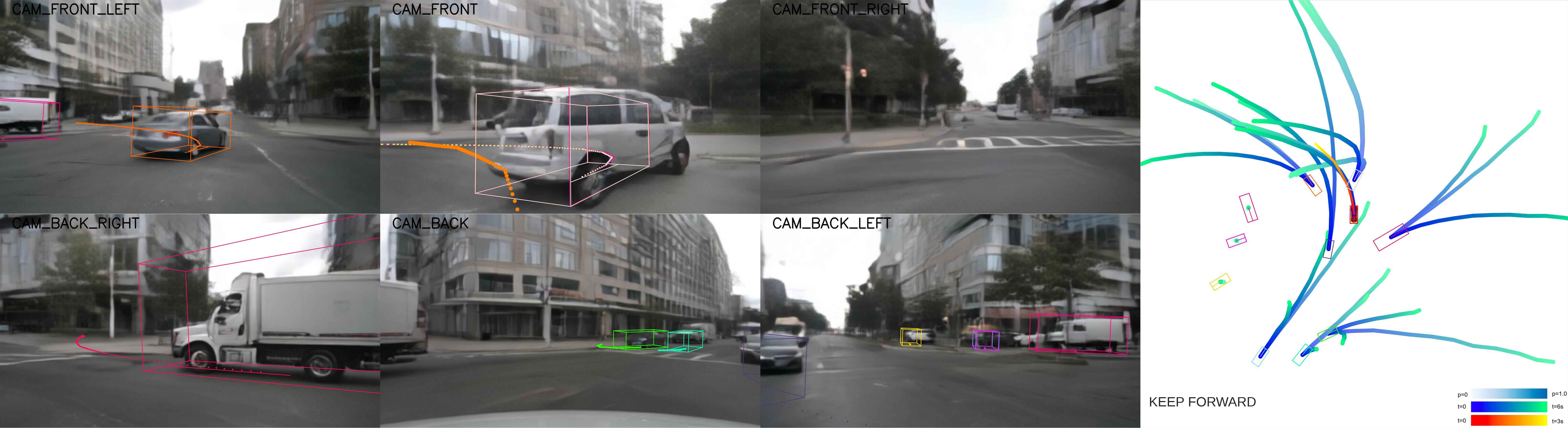
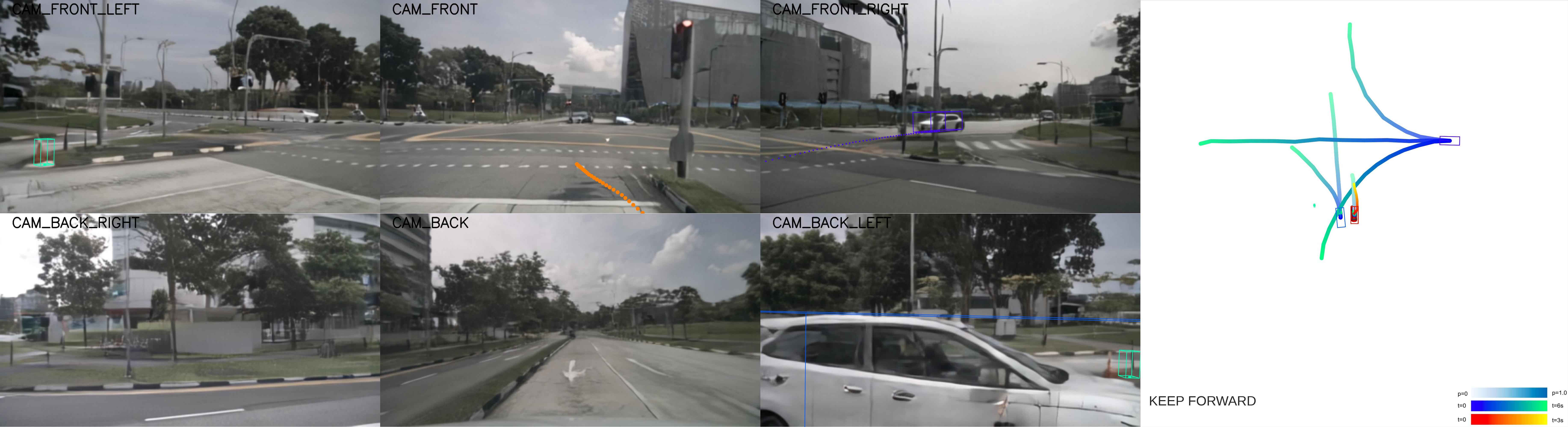
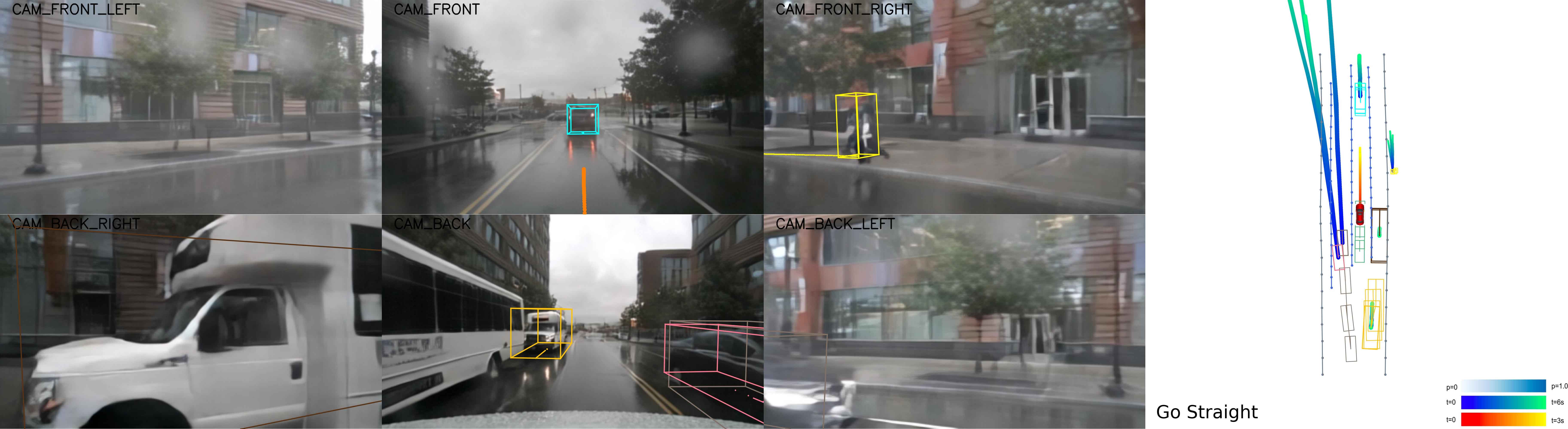
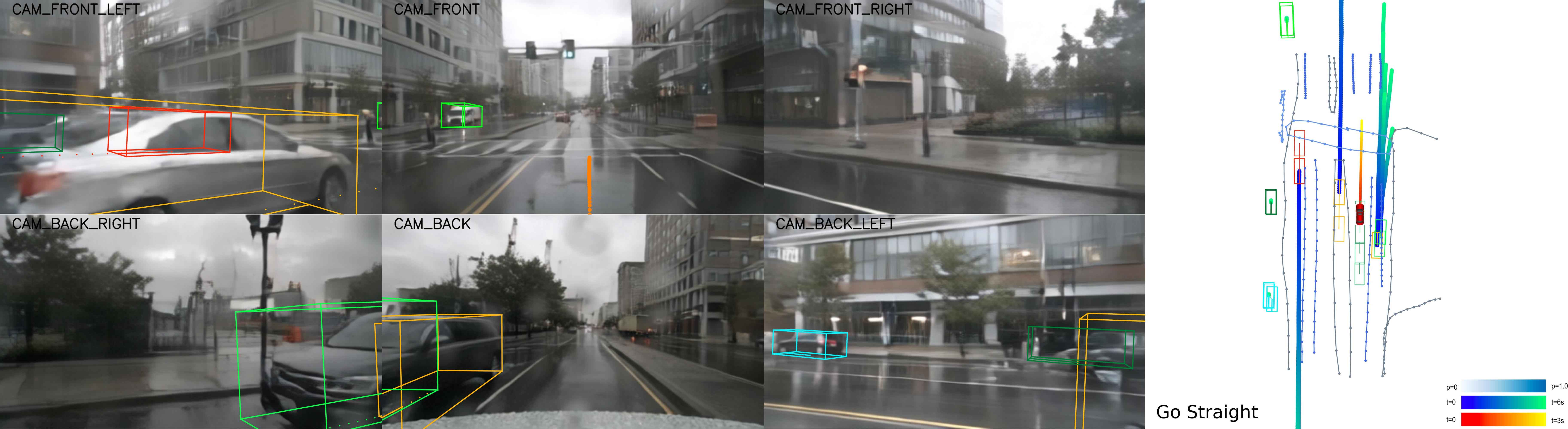
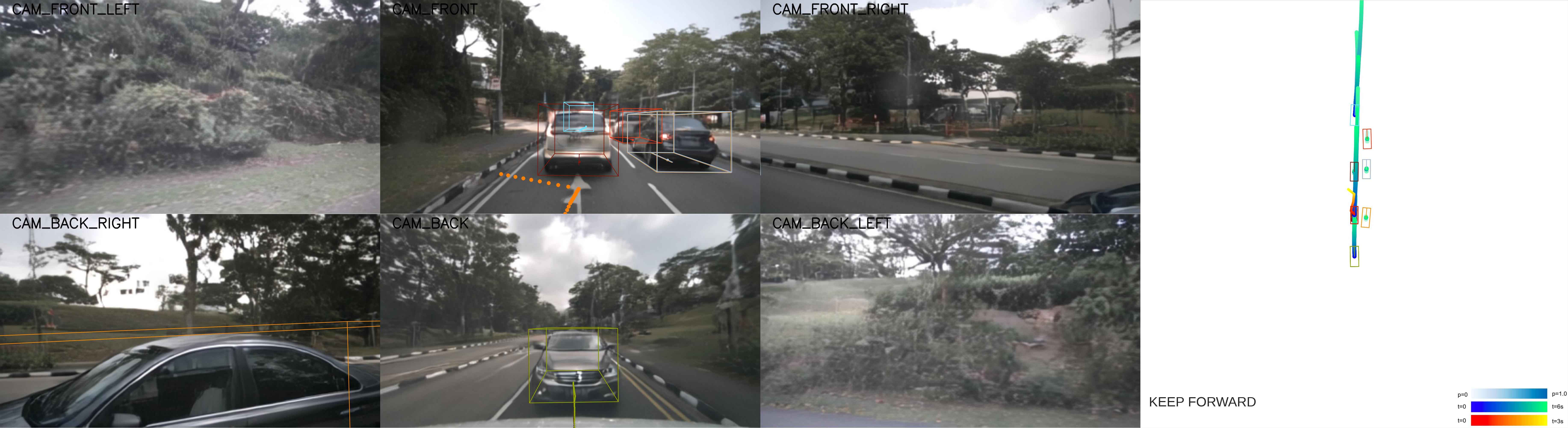
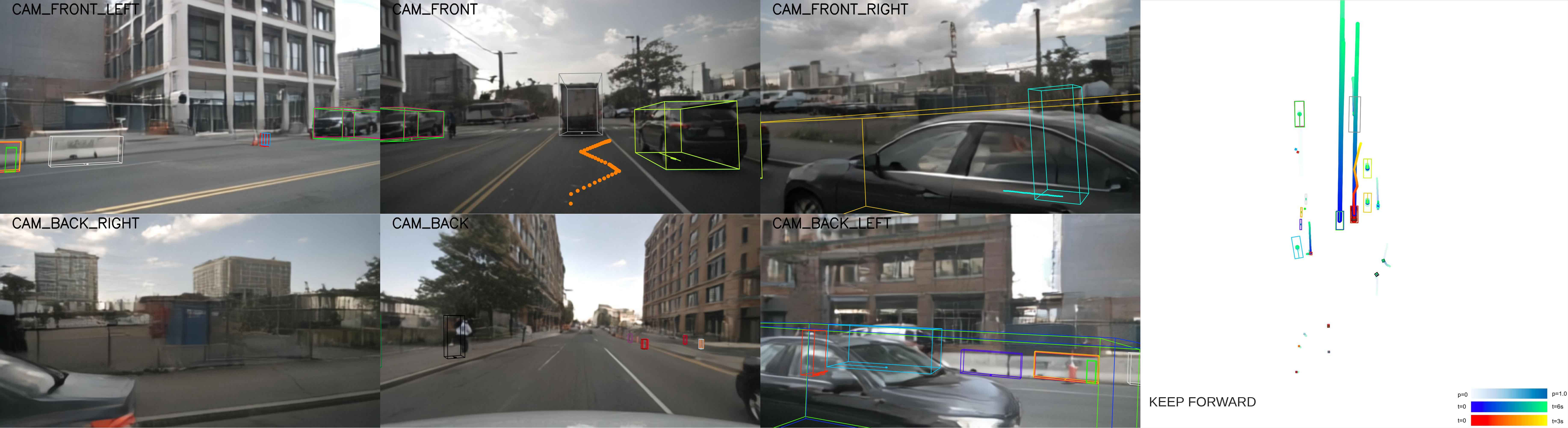
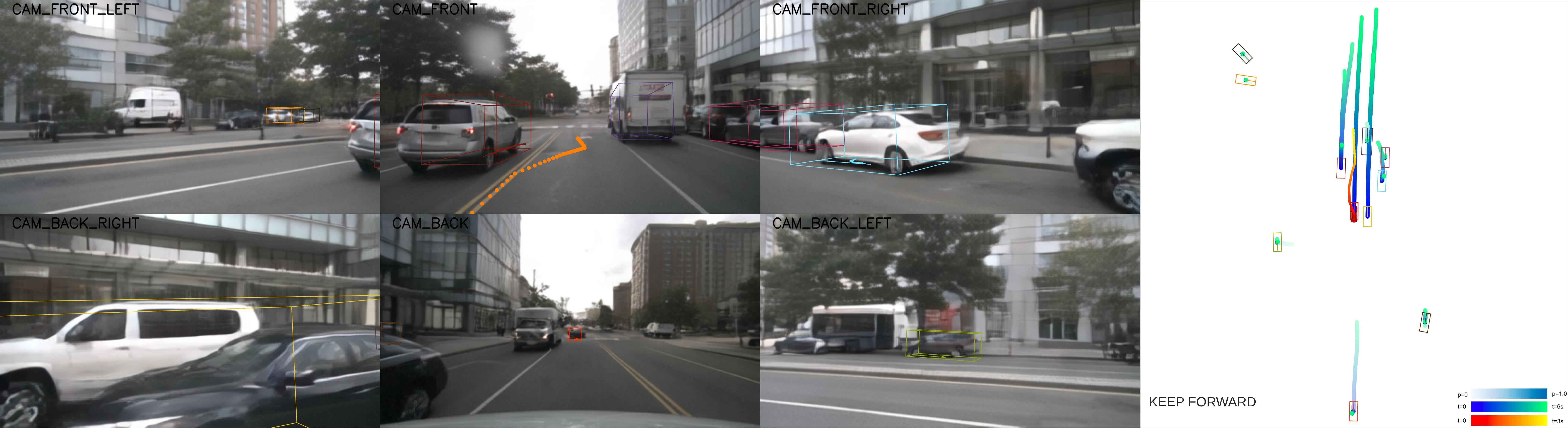
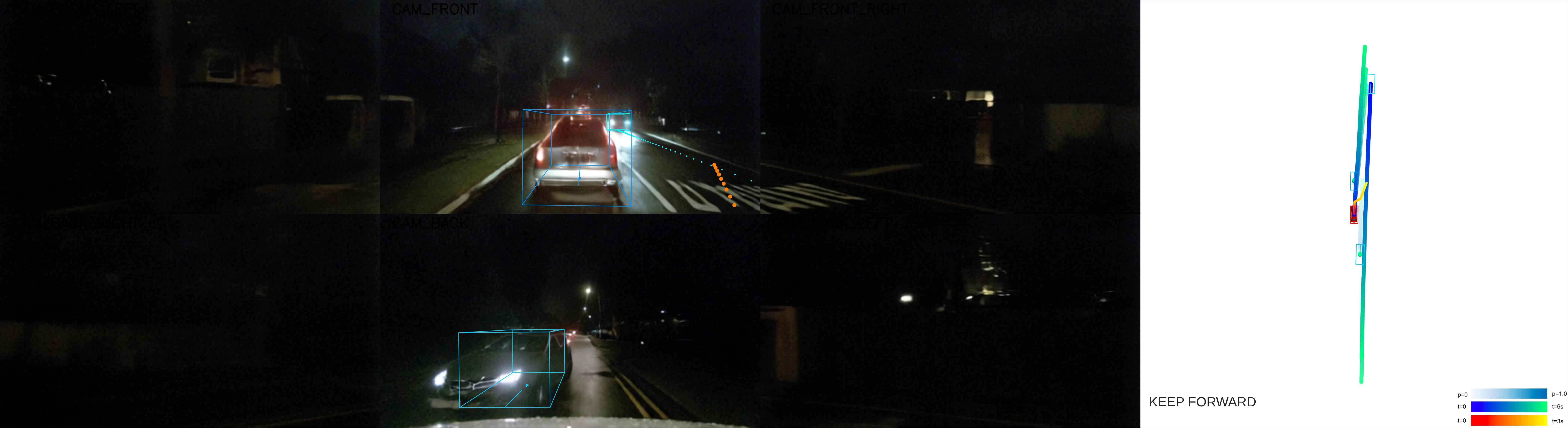
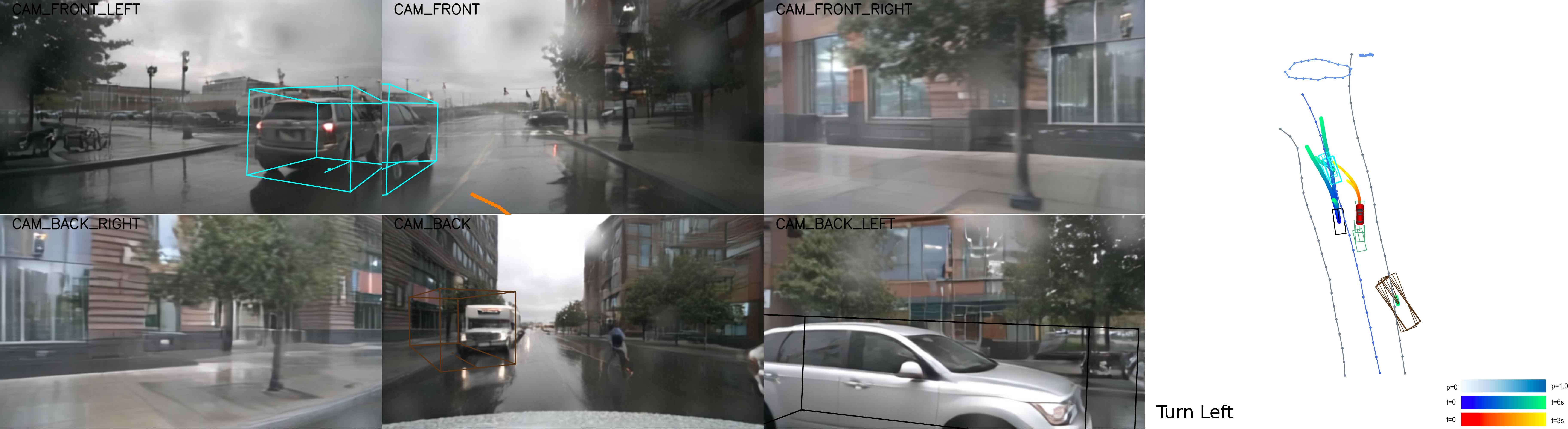
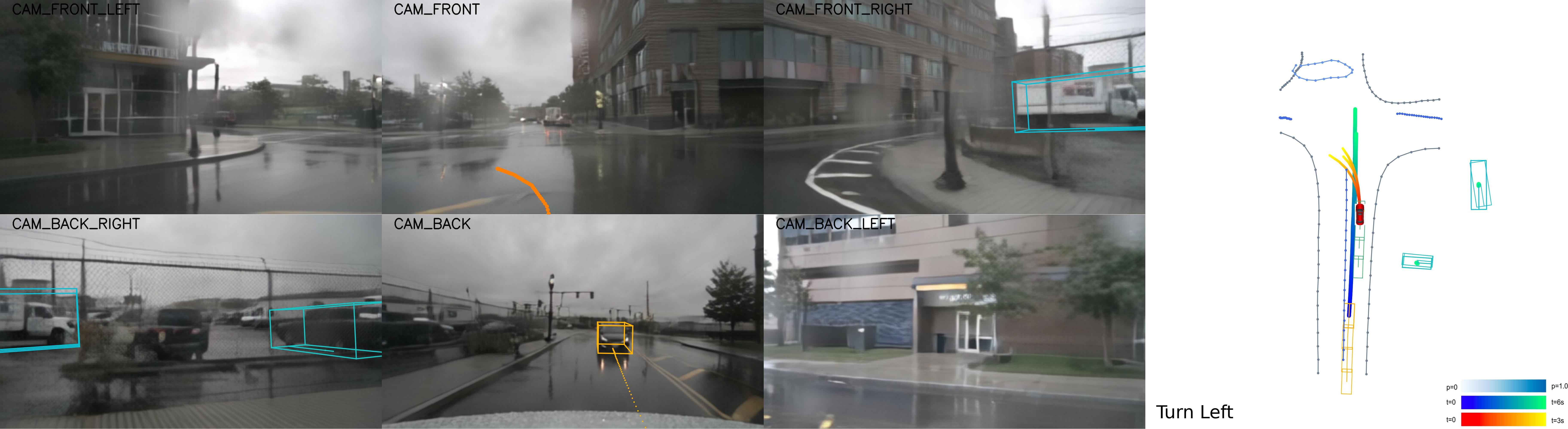
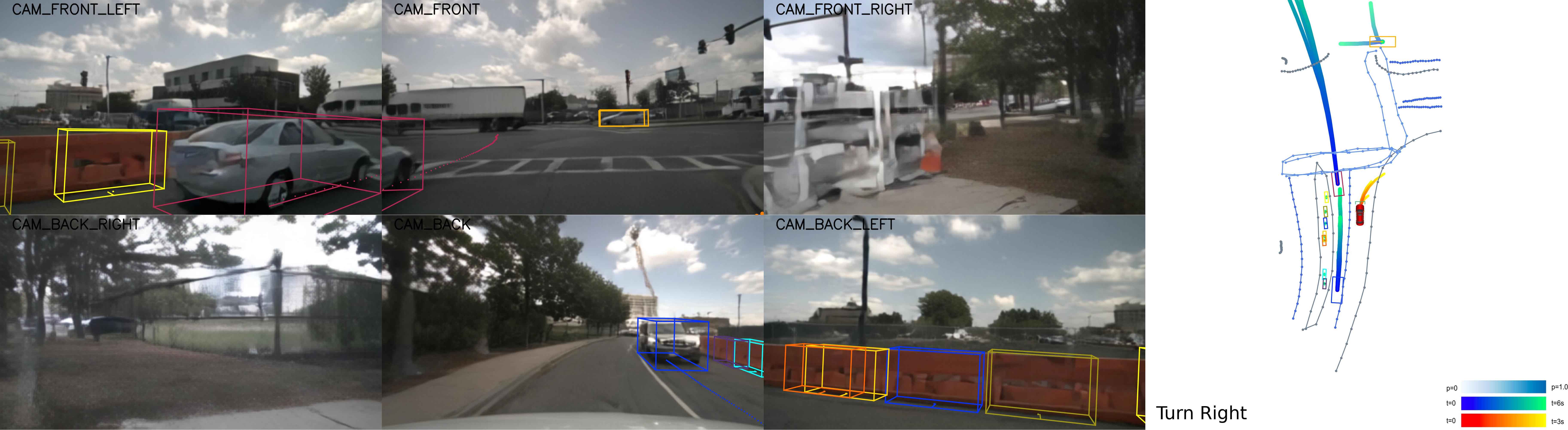
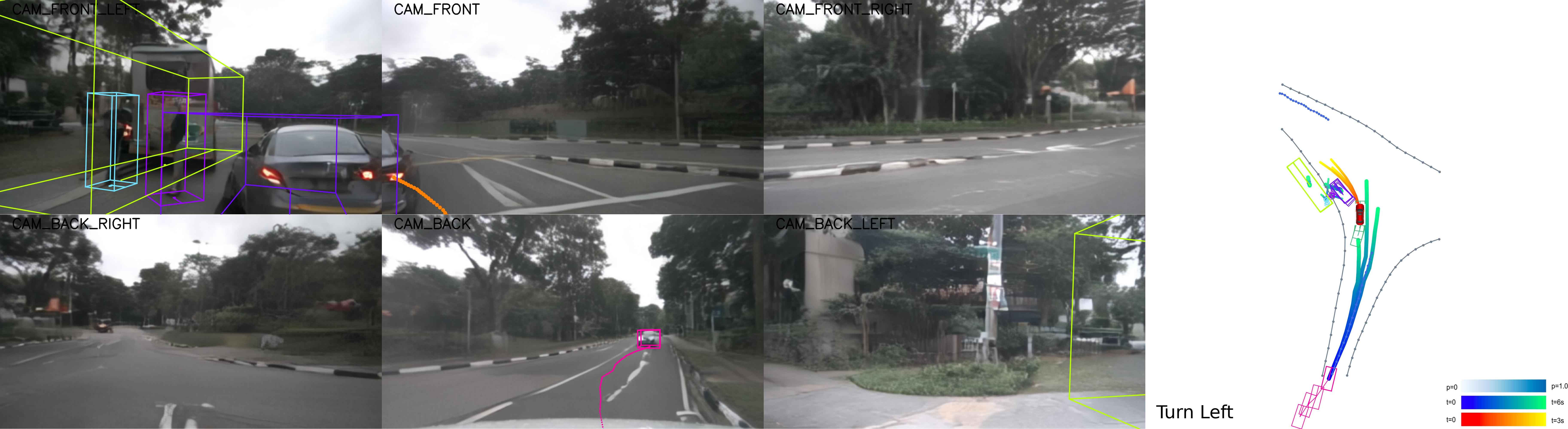
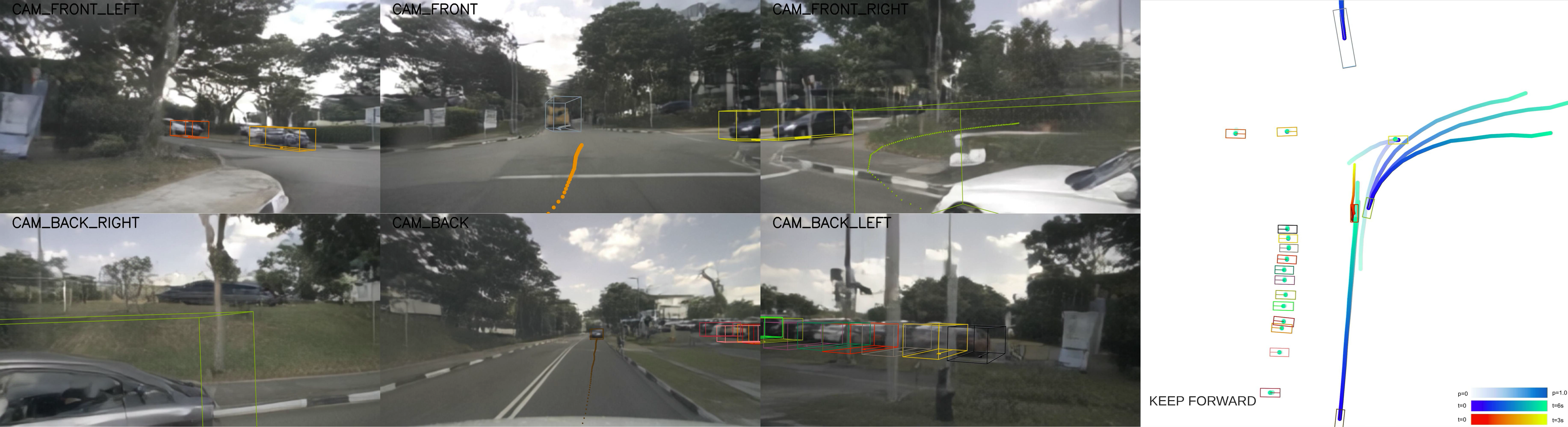
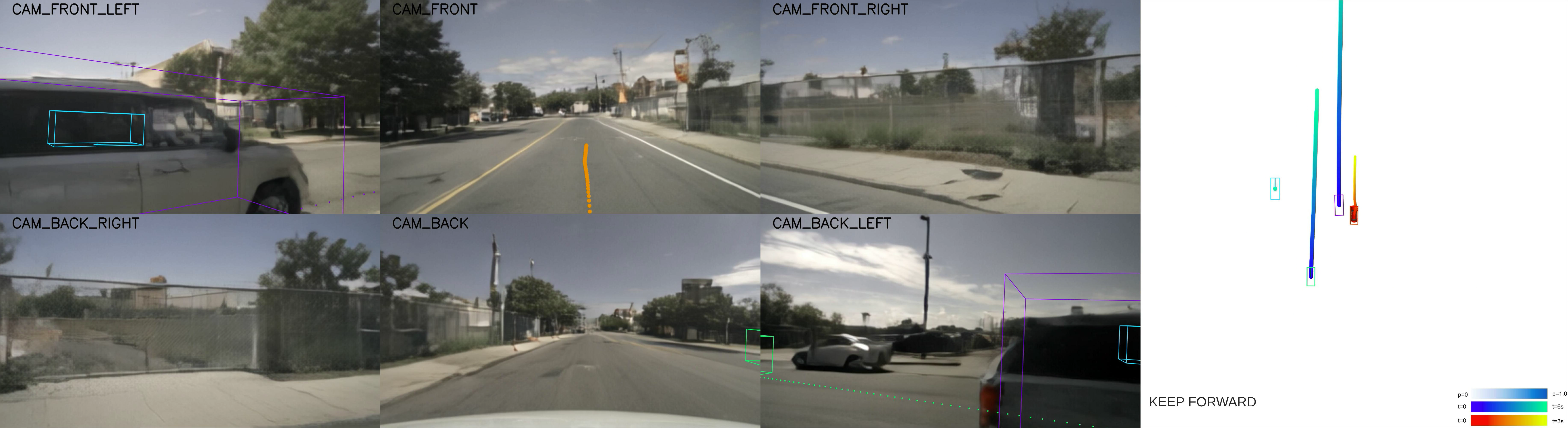
Two UniAD examples show an overtake from the right misread as a right turn, and a left cut-in misread as continued straight motion. The generated traffic therefore exposes mismatches between predicted and actual agent trajectories. Training-data bias is the authors’ proposed explanation, not a directly measured cause in these examples.
4.4 Attack Transferability
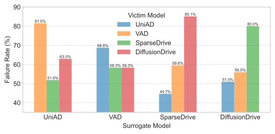
For each surrogate model, retain scenes in which it predicts a collision in at least one sample, then measure how often another model also fails in at least one sample. The plotted off-diagonal scene-level rates range from 44.7% to 85.1%. These conditional transfer rates differ from the per-sample collision rates in the main table and do not describe random unfiltered scenes.
4.5 Ablation Study.
On twenty selected validation scenes, full Challenger produces a 6.17% failure rate for UniAD, versus 3.49% without multiround refinement, 0.13% without trajectory scoring, and 0.80% without either component. Scoring is essential in this comparison, while refinement further raises difficulty. The non-monotonic no-scoring variants and limited scene subset caution against interpreting these results as a universal independent contribution of each module.
4.6 Video Quality Evaluation
Vehicle-focused subject consistency is 0.8349 on original imagery, 0.8173 on unchanged re-rendering, and 0.8093 on Adv-nuSc. Imaging quality is 0.3801, 0.3471, and 0.3469 respectively. These diagnostics reveal a rendering gap despite convincing examples. They assess generated appearance and temporal coherence, not exact physical fidelity or a calibrated probability of real-world failure.
5 Conclusion
Searching traffic motion before rendering makes sensor-level adversarial testing practical and reveals substantial vulnerabilities in the evaluated open-loop planners. The results support using generated scenarios as additional stress tests, while leaving closed-loop behavior and transfer to real traffic unmeasured.
6 Limitations
The renderer can introduce artifacts and distribution shift. Evaluation is limited to open-loop, vision-based end-to-end systems; closed-loop interaction and additional modalities such as lidar remain future work. The simplified vehicle simulation, geometric difficulty proxy, and collision-free reference-path check also limit the safety conclusions that can be drawn.
Appendix
The appendix specifies scoring, refinement, hyperparameters, runtime, video-quality measurement, dataset construction, multiple adversarial vehicles, and further failure examples.
Appendix A Implementation Details
Algorithm 1 gives the full scene-generation loop. The appendix supplies exact scoring and sampling formulas and fixed parameter values; its score convention must be reconciled with the algorithm’s maximization notation.
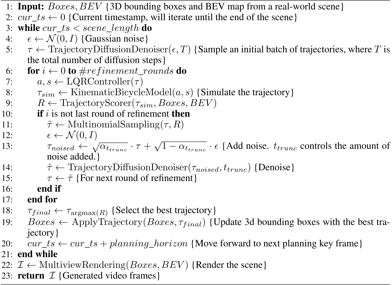
The algorithm takes 3D bounding boxes and a BEV map from a real-world scene as input, and makes adversarial driving plans for an adversarial vehicle periodically. On each planning key frame, a multi-round trajectory refinement process is performed, and the final trajectory is used to update the 3D bounding boxes. The algorithm then renders the scene using the updated bounding boxes and BEV map.
A.1 Trajectory Scoring
Lower scores are preferred. Drivable-space penalties use the center and four corners of each vehicle box, penalizing center violations more than corner violations. Collision checks combine distance screening with box intersections. Time weights emphasize early road or collision violations, while the proximity term gives more weight to later close approaches.
The final objective weights road violations, collisions, and normalized ego distance by 5, 10, and 1, with a small random initialization. The displayed normalization divides by the within-batch distance-score range; behavior when that range is zero is not specified. These choices discourage pre-existing crashes, which neither the kinematic simulator nor the renderer is designed to represent.
Equations
A.2 Multi-round Trajectory Refinement
Multinomial resampling uses softmax of negative score multiplied by a temperature parameter. Under this specific convention, increasing temperature sharpens selection and decreasing it promotes diversity—the reverse of formulas that divide logits by temperature. Subsequent partial noising and denoising explore around selected motions.
Equation
A.3 Hyperparameters
The reported configuration uses twelve planning timesteps, five refinement rounds, temperature 1, initialization scale 0.001, and corner weight 0.2. Road and collision time weights decline from 1.0 to 0.85; proximity weights increase from 0.7 to 1.0. Settings are fixed across experiments except ablations and were chosen empirically without exhaustive search.
| Hyperparameter | Value |
|---|---|
| InitScale | 1e-3 |
| CornerWeight | 0.2 |
| H (planning horizon) | 12 timesteps |
| DACStepWeight | Quadratically decreasing from 1.0 to 0.85 |
| ColStepWeight | Quadratically decreasing from 1.0 to 0.85 |
| ACStepWeight | Linearly increasing from 0.7 to 1.0 |
| DACWeight | 5 |
| CRWeight | 10 |
| ACWeight | 1 |
| Temperature | 1.0 |
| #Refinement Rounds | 5 |
Appendix B Runtime Analysis
A typical six-view, roughly 240-frame scene takes 818.62 seconds on a server with two Xeon Platinum 8457C processors, four 48 GB NVIDIA L20 GPUs, and 512 GB RAM. Sampling takes 17.36 seconds, physics 211.36, scoring 194.72, and rendering 395.18. Trajectory sampling uses one GPU; rendering uses all four, while physics and scoring are CPU-bound. This is offline generation, about 13.6 minutes per scene on the stated hardware. Avoiding rendering each candidate is the principal cost-saving design; proposed GPU optimization of scoring is future work.
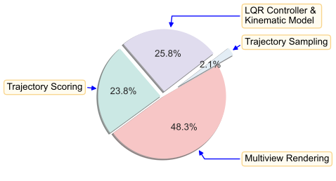
| Component | Runtime (s) |
|---|---|
| Traj. Sampling | 17.36 |
| Physics | 211.36 |
| Traj. Scoring | 194.72 |
| Rendering | 395.18 |
| Total | 818.62 |
Appendix C Video Quality Evaluation
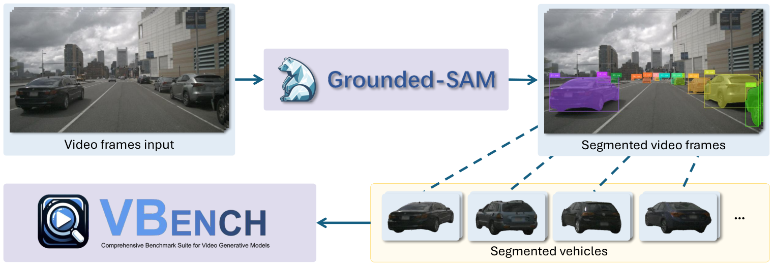
The adapted VBench [68] protocol uses Grounded-SAM 2 with a car prompt, filters masks against projected three-dimensional annotations, then measures imaging quality and subject consistency for retained vehicles. This accommodates multiple changing subjects better than a single persistent-subject assumption. It remains annotation-assisted and vehicle-focused, so it does not independently validate the entire rendered environment.
Appendix D The Adv-nuSc Dataset
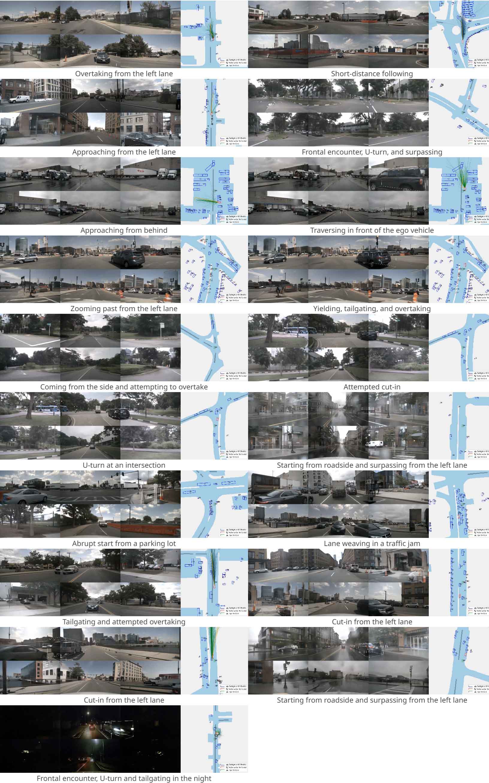
For each base scene, up to ten nearby background vehicles become candidate adversarial agents. Filtering removes collisions, departures from a 100-by-100-meter ego-centered area, and agents that never approach the ego vehicle. Remaining scenes are ranked by challenge before rendering, with manual inspection of a subset. The final dataset contains 156 scenes, 6,115 samples, 12,858 instances, and 225,085 annotations; it is a selected stress-test distribution rather than an estimate of natural event frequency.
| Attribute | Count |
|---|---|
| # instances | 12,858 |
| # ego poses | 254,436 |
| # scenes | 156 |
| # samples | 6,115 |
| # sample data | 254,436 |
| # annotations | 225,085 |
Appendix E Extending to Multiple Adversarial Vehicles
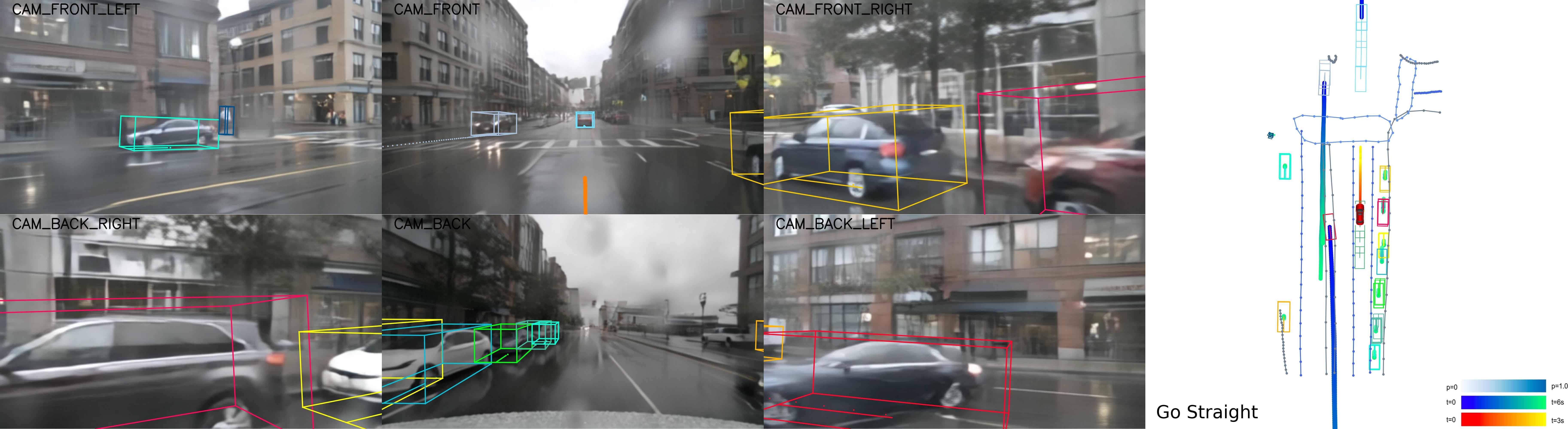
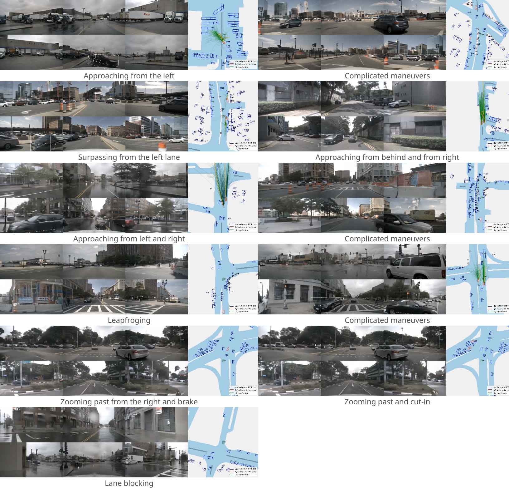
Multiple adversaries are added sequentially: generate one vehicle’s motion, feed the modified scene back into the pipeline, and choose another vehicle while treating earlier plans as fixed environment motion. Rendering occurs after all additions. The examples show richer simultaneous threats, but the method does not jointly model adversaries’ semantic coordination or solve a coupled multi-agent optimization.

Appendix F Additional Qualitative Results
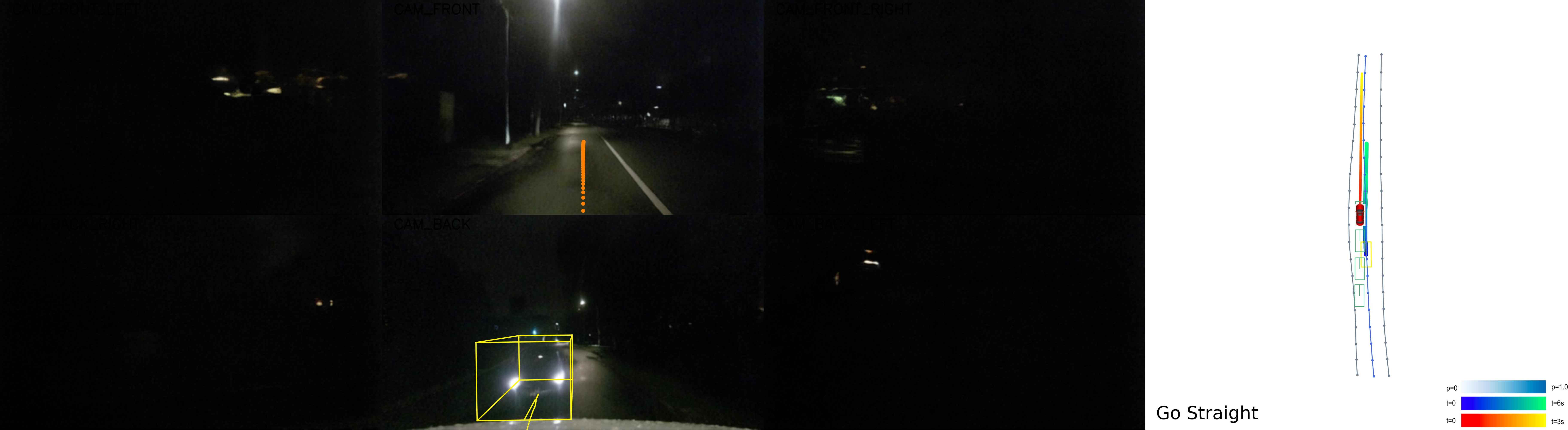
Additional UniAD and SparseDrive examples distinguish misforecasting from misplanning. In the first, other vehicles’ overtakes, cut-ins, blocking, or U-turns are predicted incorrectly. In the second, unsafe ego plans appear despite reasonably informative forecasts, including turns into occupied lanes or curbs. These manually selected cases illustrate failure types; they do not quantify their prevalence or establish which training change would eliminate them.