Overview
The opening figure links condition-sensitive hidden representations to faster benchmark learning. The complete model diagram, learning curves, rollout examples, five numbered tables, both theoretical results, all equations and original pseudocode are retained.
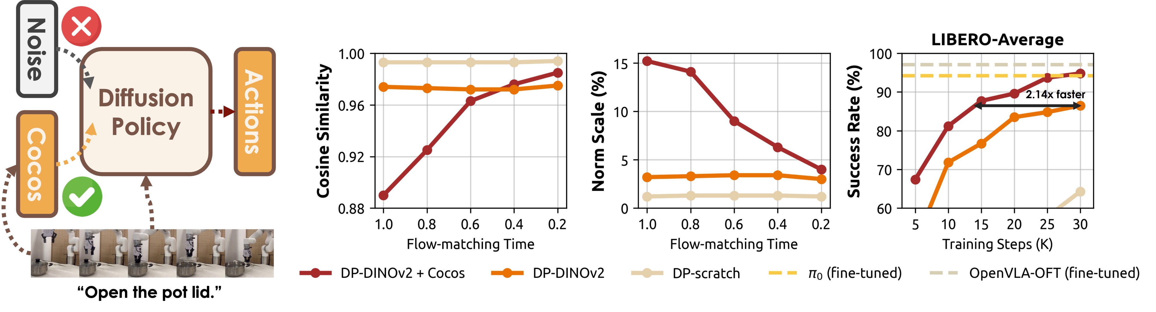
At a glance
Cocos changes a diffusion policy’s initial noise distribution from a condition-independent Gaussian to one centered on compressed visual-language features. The policy still receives the usual conditioning inputs. On a compact flow-matching Transformer, the change raises LIBERO average success from 86.5% to 94.8% and MetaWorld from 59.5% to 74.8%, with favorable learning curves and real-robot results. The theoretical analysis identifies conditions under which gradients become similar, but does not establish that every conditional prior prevents collapse or guarantee global training convergence.
1 Introduction
A policy can generate plausible actions while using visual or language inputs poorly. The authors observe weaker changes in hidden states when conditions are injected into weaker policies, and call the tendency to fit marginal actions instead of condition-specific behavior “loss collapse.” These representation diagnostics correlate with success; they do not directly measure instruction comprehension or prove a single cause of every failure.
Cocos makes the source action-shaped noise itself depend on the condition, while keeping the existing policy conditioning pathway. Its contribution is an inexpensive change to the generative training setup, rather than a new large vision-language model. Experiments cover 40 LIBERO and 30 MetaWorld tasks plus ten tasks on each of two physical robots. Claims of architecture-wide compatibility extend beyond the one compact RDT recipe tested here.
2 Preliminaries
The policy imitates demonstrated action chunks conditioned on encoded images and language. Flow matching [12] learns a time-dependent velocity that transports an initial distribution into an action distribution. Conditional flow matching trains on tractable source-target interpolation paths; averaging their velocities with the appropriate density weights recovers the marginal transport field. The term “conditional” in this construction refers to the interpolation endpoints and should be distinguished from the robot’s observation/instruction condition.
Equations 1–3
| (1) |
| (2) |
| (3) |
3 How Generative Conditions Can Lead to Loss Collapse
The analysis asks when a velocity network may fail to distinguish different observation or instruction conditions. Its exact assumptions and proof steps remain available with the original statements.
3.1 Flow with Generative Conditions
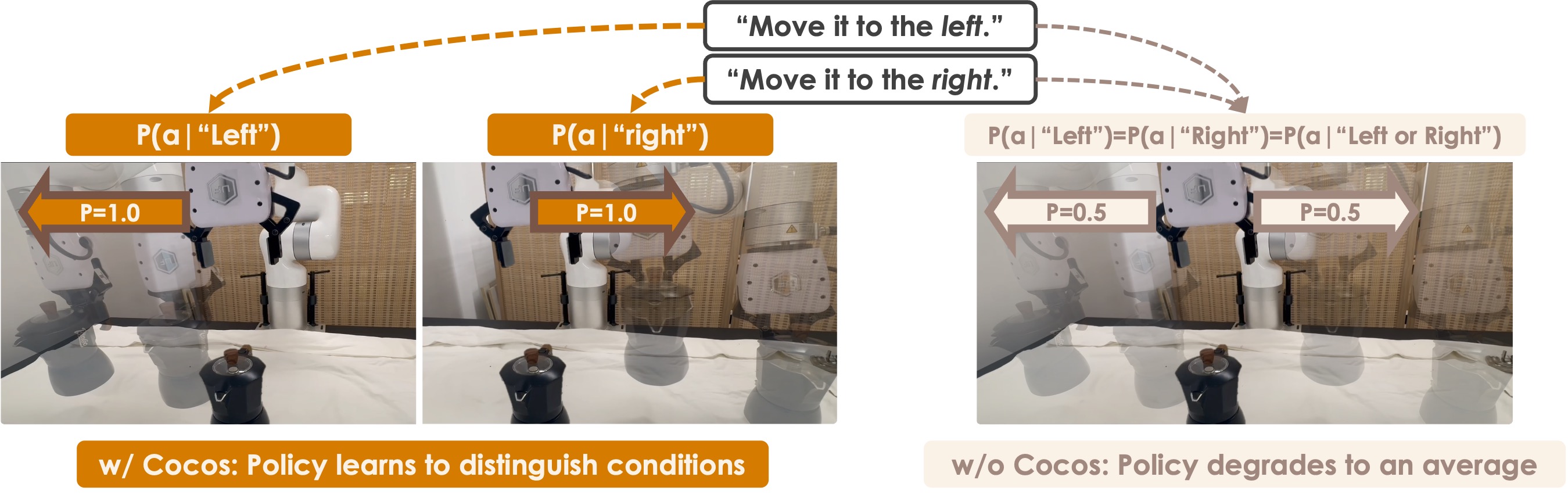
Introducing a generative condition yields a condition-specific probability path and target velocity. Lemma 1 relates squared error against the marginal conditional field to squared error against endpoint-conditioned fields, up to an additive parameter-independent constant, assuming positive densities and the regularity conditions supplied in Appendix A. Standard training samples a condition-action pair and independent Gaussian source noise, then predicts the interpolation velocity. Figure 3 illustrates indistinguishable left/right instructions; it is a conceptual mechanism illustration, not a separate quantitative experiment.
Equations 4–7
| (4) |
| (5) |
| (6) |
| (7) |
3.2 Loss Collapse
Theorem 1 assumes bounded network Jacobian M, bounded velocity residual D, outputs differing by at most ε across conditions, and an additional output-sensitive Lipschitz bound K on the Jacobian. Under a common sampling measure, the parameter-gradient difference is at most 2(M + KD)ε. This explains how already similar outputs and Jacobians can yield similar updates. It does not establish that all ordinary diffusion policies satisfy these strong assumptions, nor that gradient descent must converge to a condition-independent optimum.
Changing the source distribution adds a difference between sampling measures, so the same O(ε) contraction need not follow. That absence of a small upper bound is not a positive lower bound on useful conditioning: a conditional prior may still be uninformative or nearly identical across conditions. The proof’s “arbitrarily large” claim also needs qualification under its own uniform boundedness assumptions; Appendix A notes the issue explicitly.
Equations
4 Method
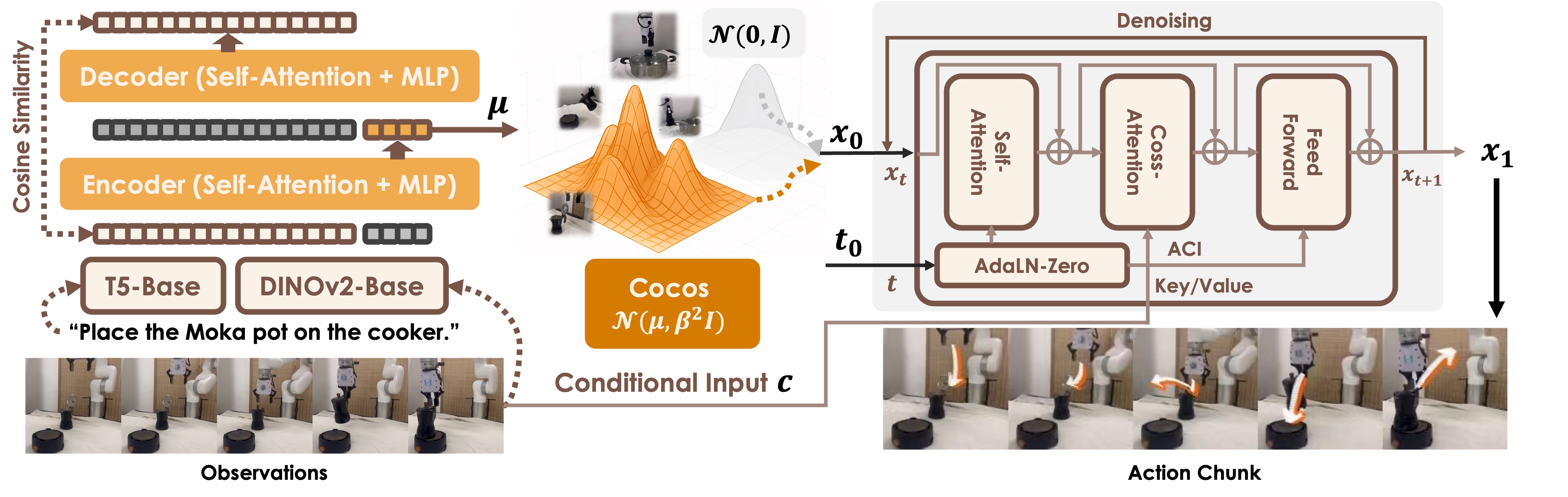
Cocos samples source actions from a Gaussian with mean αFϕ(E(c)) and covariance β²I. The feature encoder maps frozen condition embeddings to the action dimensionality; α controls mean strength and β noise scale. Setting α = 0 and β = 1 recovers the standard prior. Both training and inference must sample from the same condition-dependent source.
A small encoder-decoder is trained to reconstruct condition embeddings using negative cosine similarity. The default first trains this autoencoder and then freezes it during policy training. A joint variant instead uses an exponential moving average of the encoder to slow changes to the source distribution. The policy follows a linear interpolation schedule with target velocity x₁ − x₀ and retains its ordinary cross-attention conditioning.
Algorithm 1 is preserved exactly. Its printed update uses θ ← θ + ∇θL without a negative sign or learning rate, despite a squared-error minimization objective; it should be treated as schematic pseudocode rather than executed literally. The theory motivates changed sampling but does not prove that reconstruction-trained features always encode the task distinctions that control requires.
Equations 8–10
| (8) |
| (9) |
| (10) |
5 Experiments
The experiments test learning speed and final success, real-robot behavior, and qualitative conditioning failures. The section labels swap RQ2 and RQ3 relative to the initial question list; the experiment content is unambiguous.
5.1 Experimental Setup
The policy network is a roughly 40-million-parameter compact RDT [15]. Frozen DINOv2-Base [20] and T5-Base [25] encode vision and language; the source autoencoder has one Transformer layer in each encoder/decoder. Comparisons are DP-scratch without pretrained vision, DP-DINOv2 with ordinary source noise, and DP-DINOv2 with Cocos. The 40M count describes the policy backbone, not the total size including frozen encoders and source autoencoder.
LIBERO [13] evaluates four ten-task suites; MetaWorld [34] uses 30 selected tasks. SO100 and xArm each supply ten physical tasks. Simulation reports 150 evaluation trials per task, described as 50 trials at each of three random seeds. The text does not clearly identify independent training runs or define every ± statistic as standard deviation versus standard error.
5.2 Overall Comparison (RQ1)
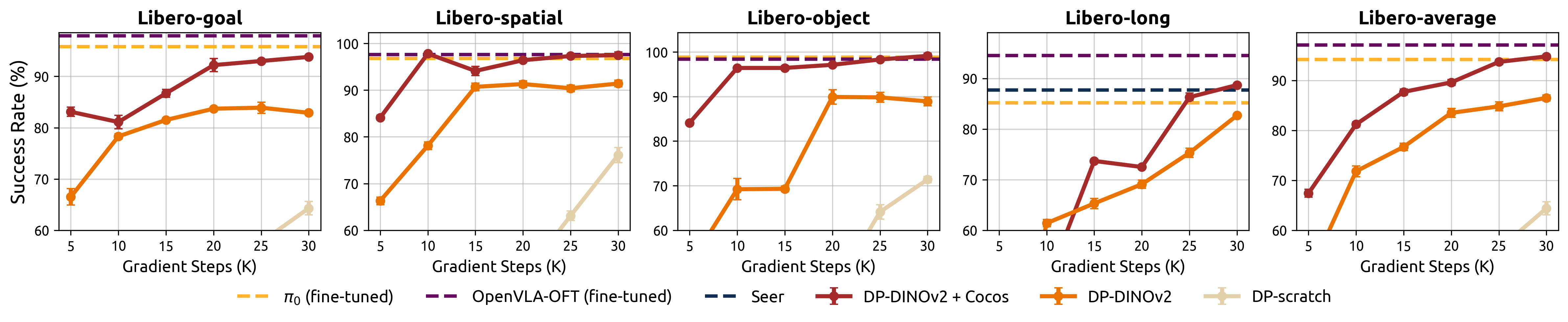
At the reported endpoint, LIBERO averages are 64.4% for scratch, 86.5% for DINOv2 and 94.8% for default Cocos: an 8.3-percentage-point gain. Goal/Spatial/Object/Long success for Cocos is 93.8/97.5/99.1/88.7%. The learning curves improve early and the paper reports 2.14× faster convergence. This is a gradient-step comparison, not a measured 2.14× reduction in wall time, GPU-hours or total cost including autoencoder training.
MetaWorld averages improve from 59.5% to 74.8%, a 15.3-point or approximately 25.7% relative increase. Gains are not universal: disassemble falls from 72.7% to 39.3%, some button tasks decline slightly, and several tasks tie. The complete task-level table is preserved so the aggregate does not conceal these differences.
Curves compare against reported fine-tuned π₀ [1], OpenVLA-OFT [10] and Seer [29] scores. Cocos reaches similar average performance within 30K policy updates; cited fine-tuning budgets are 50–150K for OpenVLA-OFT and 100–250K for π₀. Different pretrained models, data filtering, batch sizes and total pretraining/auxiliary-training costs prevent interpreting this as a controlled compute-efficiency ranking. Lower hidden-state cosine similarity and larger norm changes support greater conditioning influence, but do not isolate the causal contribution of the source prior from the explicit conditioning path.
| DP-scratch | DP-DINOv2 | Cocos (0.2 std) | Cocos (0.1 std) | Cocos (0.4 std) | Cocos (VAE) | Cocos (EMA) | ||
| LIBERO | Goal | 64.3±1.3 | 82.9±0.4 | 93.8±0.3 | 50.9±1.8 | 92.3±0.9 | 92.5±0.3 | 90.5±0.4 |
| Spatial | 76.1±1.6 | 91.4±0.7 | 97.5±0.7 | 97.1±0.4 | 96.7±0.5 | 96.1±0.7 | 97.5±0.2 | |
| Object | 71.4±0.7 | 88.9±1.0 | 99.1±0.6 | 79.3±0.8 | 97.6±1.0 | 98.1±0.7 | 96.9±0.5 | |
| Long | 45.9±1.6 | 82.7±0.2 | 88.7±0.1 | 82.7±0.5 | 89.5±0.4 | 88.2±0.6 | 87.3±0.6 | |
| Average | 64.4 | 86.5 | 94.8 | 77.5 | 94.0 | 93.8 | 93.0 | |
button-press
button-press-td
button-press-td-w
button-press-w
coffee-button
door-open
door-lock
door-unlock
drawer-close
drawer-open
Average
w/ Cocos
100.0±0.0
95.3±0.9
94.7±3.4
97.3±2.5
100.0±0.0
99.3±0.9
44.7±1.9
93.3±4.1
100.0±0.0
100.0±0.0
74.8±0.9
w/o Cocos
97.3±2.5
96.0±1.6
91.3±4.1
99.3±0.9
97.3±2.5
77.3±5.7
3.3±0.9
67.3±5.2
100.0±0.0
100.0±0.0
59.5±3.8
scratch
48.7±8.1
41.3±6.6
32.7±6.6
82.0±5.9
53.3±0.9
50.7±4.7
23.3±2.5
24.7±3.4
88.7±0.9
57.3±5.0
33.6±3.4
faucet-close
faucet-open
handle-press
handle-press-s
window-close
window-open
handle-pull
handle-pull-s
basketball
bin-picking
w/ Cocos
82.0±2.8
100.0±0.0
99.3±0.9
100.0±0.0
100.0±0.0
94.0±3.3
2.7±0.9
9.3±4.7
80.7±8.6
64.0±6.2
w/o Cocos
80.7±3.8
84.0±4.3
98.0±1.6
98.0±1.6
100.0±0.0
89.3±4.1
1.3±0.9
0.0±0.0
0.7±0.9
46.0±5.9
scratch
36.7±3.4
79.3±1.9
76.0±2.8
53.3±3.4
60.7±1.9
26.0±0.0
2.0±1.6
0.0±0.0
0.0±0.0
10.0±4.3
coffee-pull
coffee-push
dial-turn
hammer
sweep
sweep-into
soccer
shelf-place
disassemble
stick-push
w/ Cocos
79.3±6.2
60.7±5.0
60.0±2.8
76.7±6.6
72.0±8.5
66.0±8.6
14.0±3.3
26.7±0.9
39.3±1.9
94.0±4.3
w/o Cocos
72.7±4.7
55.3±5.2
24.0±4.3
72.7±1.9
9.3±2.5
20.0±3.4
14.0±0.9
3.3±2.5
72.7±4.9
12.7±1.9
scratch
21.3±6.8
19.3±5.7
2.7±0.9
25.3±2.5
10.0±4.9
18.0±3.3
6.7±1.9
2.7±0.9
14.7±2.5
40.0±2.8

5.3 Real-World Experiments (RQ2)
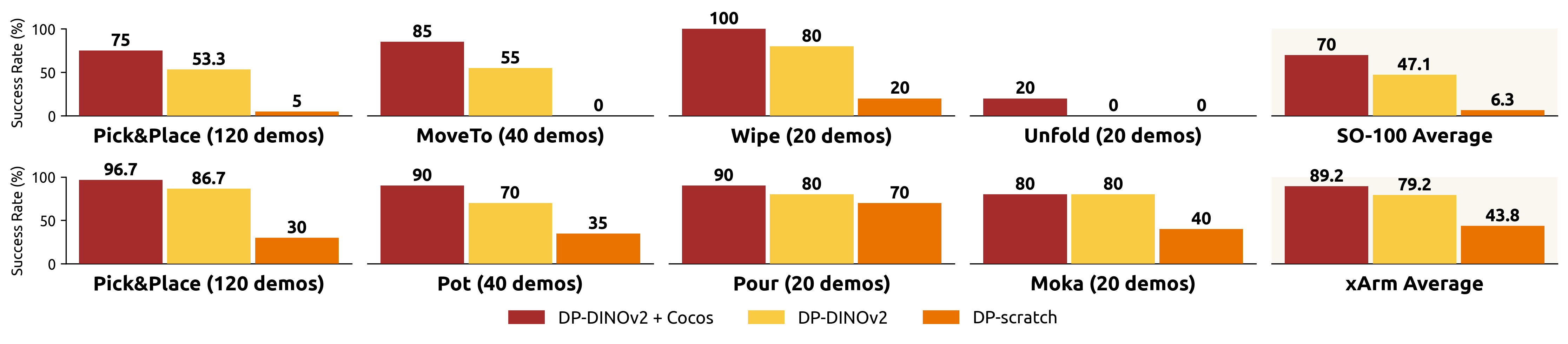
Each physical task supplies 20 demonstrations and ten test trials. Figure 5 gives SO100 suite-average success of 70.0% for Cocos, 47.1% for DINOv2 and 6.3% for scratch; xArm gives 89.2/79.2/43.8%. These bars average the four suites equally, although the suites contain different numbers of tasks. They are not a uniform average over all ten tasks.
SO100 Cocos scores are 75% pickup/place, 85% move, 100% wipe and 20% unfold. xArm scores are 96.7% pickup/place, 90% lid manipulation, 90% pouring and 80% Moka placement. The last ties the DINOv2 baseline, qualifying the claim of improvement in every suite. Rollouts suggest fewer localization and spatial-reference errors, while the small test sets and absent physical-run uncertainty limit statistical conclusions.
5.4 Case Studies (RQ3)
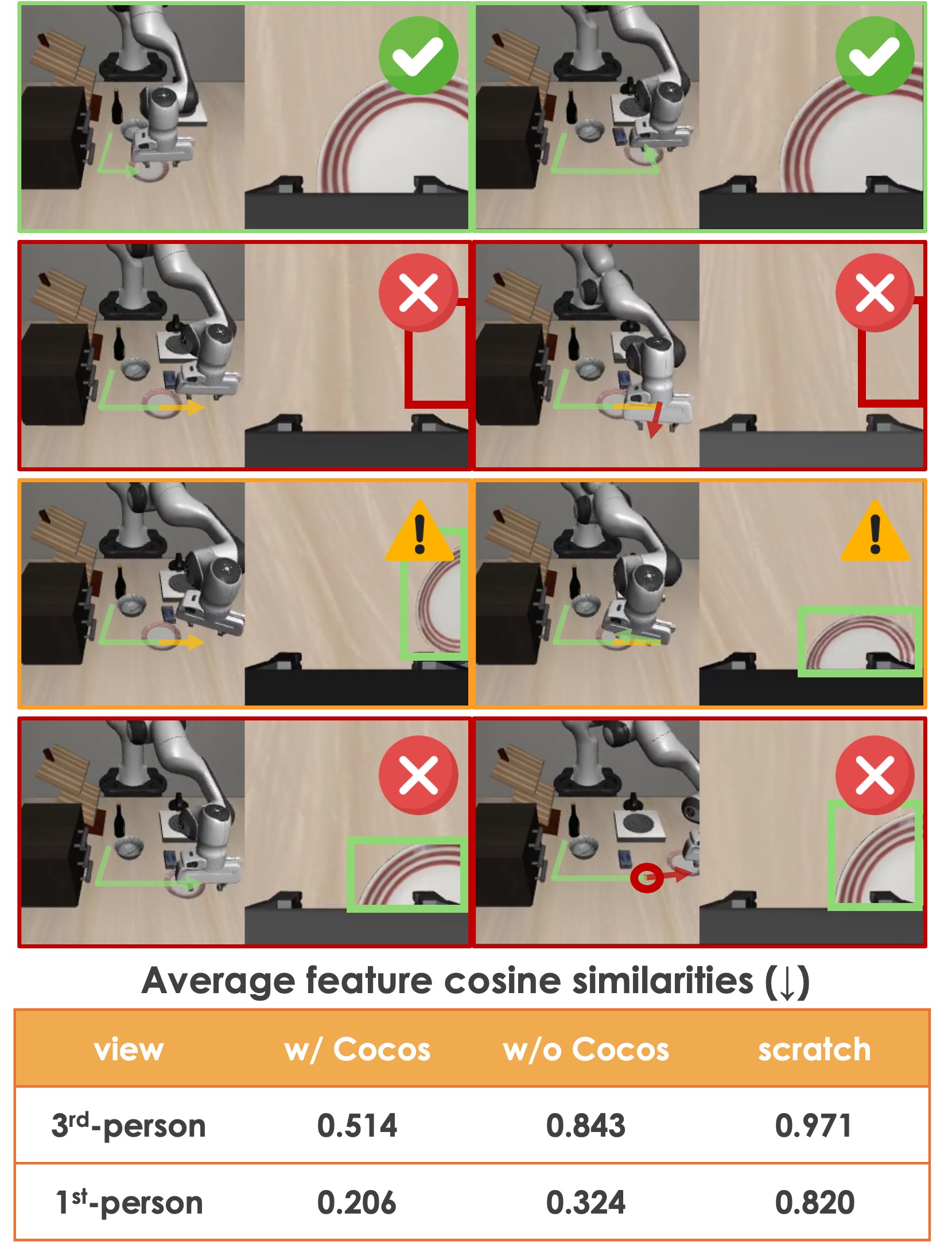
In LIBERO plate movement, selected baseline failures lose the plate outside the wrist view or push it past a stove visible in the third-person view. Cocos succeeds in the displayed comparison. Across sampled image pairs, third-person feature cosine similarity is 0.514 with Cocos versus 0.843 without and 0.971 for scratch; first-person values are 0.206/0.324/0.820. These are similarities of projected features before fusion, distinct from Figure 1’s before/after cross-attention diagnostic.
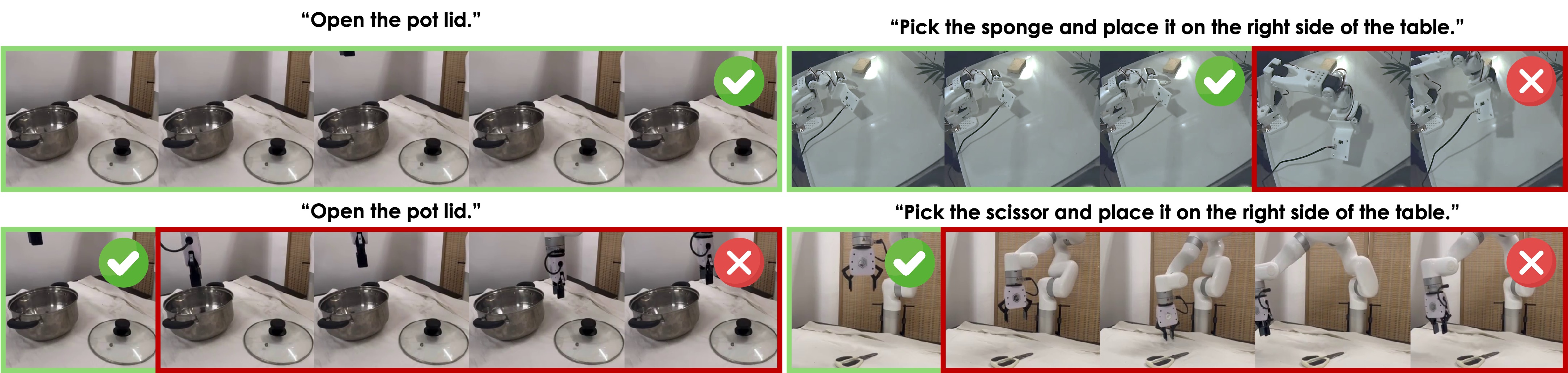
Real examples show a Cocos policy remaining idle when the requested lid-opening task is already complete, while a baseline executes unnecessary motion. Other baseline examples miss objects or confuse rightward instructions. These selected trajectories are useful failure illustrations, not randomized intervention tests proving that a particular camera or modality caused every error.
5.5 Ablation Studies
The default source standard deviation β = 0.2 reaches 94.8% LIBERO average. β = 0.4 reaches 94.0%, a learned-variance VAE variant 93.8%, and joint EMA training 93.0%. β = 0.1 drops to 77.5%, driven especially by Goal at 50.9%; narrow priors can be harmful. These few settings support a usable range rather than broad hyperparameter robustness. EMA simplifies staging with a modest lower average, and the paper supplies no significance test establishing equivalence.
6 Conclusion, Limitations, and Future Works
Condition-dependent source noise improves this compact multi-task imitation-learning recipe across several benchmarks and physical tasks. Large-scale pretraining, broad transfer and more expressive priors remain future work. Additional limits include task-level regressions, incomplete compute accounting, missing operational hyperparameters, and a theoretical conclusion stronger than the proved gradient comparison. The evidence supports Cocos as a promising practical modification, not a universal guarantee against condition omission.
Appendix A Proofs of Theorems
The lemma proof expands the two squared errors and matches the parameter-dependent terms using the density-weighted conditional velocity. It requires sufficient tail decay and bounded fields/derivatives to exchange integration and differentiation. Equal gradients imply objectives differing by a constant, as the lemma states; the final proof sentence’s claim that they are simply “equal” omits that qualification.
The theorem writes the residual d = vθ − u and f = (∇θvθ)ᵀd, then uses triangle inequalities and the Jacobian assumptions to obtain 2(M + KD)ε under a common normalized sampling measure. Its notation writes q(x₁,c) inside a measure called independent of the particular c; interpreting c as an integrated training-condition variable rather than the compared query condition is essential. Ordinary data generally has condition-dependent targets, so this notation should be resolved before applying the result as a general training theorem.
Under different measures, the gradient difference splits into a same-measure term bounded by O(ε) and a measure-change term T₁. The proof gives no lower bound on T₁ and no convergence analysis. Moreover, its uniform bounds imply ‖f‖ ≤ MD and therefore ‖T₁‖ ≤ 4MD for probability measures, contradicting literal unbounded growth while fixed M and D remain in force. A dependence not controlled by ε is the defensible conclusion; guaranteed escape from collapse does not follow. Every original equation and theorem statement remains unchanged.
Equations 11–41
| (11) |
| (12) |
| (13) | ||||
| (14) | ||||
| (15) |
| (16) | ||||
| (17) | ||||
| (18) | ||||
| (19) | ||||
| (20) |
| (21) |
| (22) |
| (23) |
| (24) |
| (25) |
| (26) |
| (27) | ||||
| (28) | ||||
| (29) |
| (30) | ||||
| (31) | ||||
| (32) |
| (33) | ||||
| (34) |
| (35) |
| (36) |
| (37) | ||||
| (38) | ||||
| (39) | ||||
| (40) |
| (41) |
Appendix B Details of Benchmarks
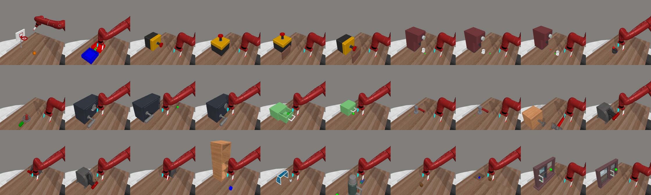
LIBERO has four ten-task suites with 500 demonstrations per suite; unsuccessful demonstrations are retained, unlike some cited comparison protocols. Policies observe current two-view RGB images, predict 16 actions and execute eight before replanning. MetaWorld uses 20 scripted demonstrations for each of 30 selected tasks, one current RGB view, 16 predicted actions and all 16 executed. Both evaluate 50 trials at three random seeds. Tables 3–4 retain all 70 task descriptions.
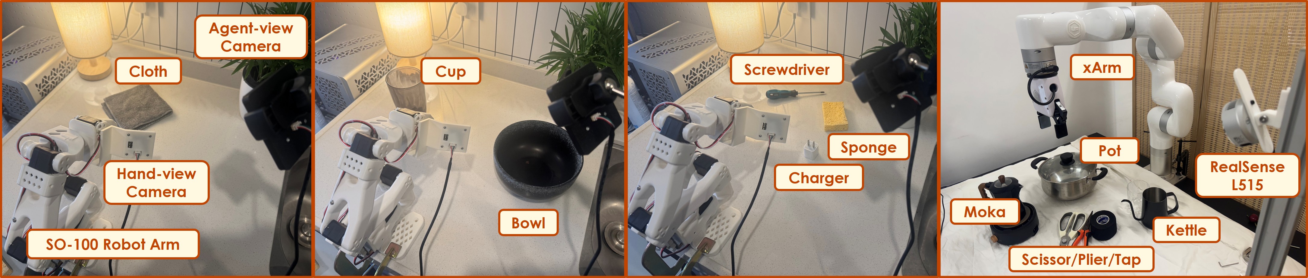
SO100 uses two 640×480 cameras at 25 FPS and a 30 Hz controller; xArm uses a third-person L515 at 30 FPS and a 30 Hz controller. Both predict absolute joint-angle chunks of length 64 and execute 40 steps. Observations include current RGB images and current plus ten prior joint states. Although xArm records depth, the stated policy observation is RGB plus joints; depth use is not demonstrated.
Each robot’s ten tasks comprise six object/placement combinations and four other tasks. SO100 adds two move tasks, wiping and unfolding; xArm adds lid opening/closing, pouring and Moka placement. Table 5 retains exact instructions and parameter combinations. SO100 jitter, limited payload and camera lag are acknowledged hardware constraints.

| Task Suite | Task Description |
| LIBERO-Goal | open the middle layer of the drawer |
| put the bowl on the stove | |
| put the wine bottle on the top of the drawer | |
| open the top layer of the drawer and put the bowl inside | |
| put the bowl on the top of the drawer | |
| push the plate to the front of the stove | |
| put the cream cheese on the bowl | |
| turn on the stove | |
| put the bowl on the plate | |
| put the wine bottle on the rack | |
| LIBERO-Spatial | pick the akita black bowl between the plate and the ramekin and place it on the plate |
| pick the akita black bowl next to the ramekin and place it on the plate | |
| pick the akita black bowl from table center and place it on the plate | |
| pick the akita black bowl on the cookies box and place it on the plate | |
| pick the akita black bowl in the top layer of the wooden cabinet and place it on the plate | |
| pick the akita black bowl on the ramekin and place it on the plate | |
| pick the akita black bowl next to the cookies box and place it on the plate | |
| pick the akita black bowl on the stove and place it on the plate | |
| pick the akita black bowl next to the plate and place it on the plate | |
| pick the akita black bowl on the wooden cabinet and place it on the plate | |
| LIBERO-Object | pick the alphabet soup and place it in the basket |
| pick the cream cheese and place it in the basket | |
| pick the salad dressing and place it in the basket | |
| pick the bbq sauce and place it in the basket | |
| pick the ketchup and place it in the basket | |
| pick the tomato sauce and place it in the basket | |
| pick the butter and place it in the basket | |
| pick the milk and place it in the basket | |
| pick the chocolate pudding and place it in the basket | |
| pick the orange juice and place it in the basket | |
| LIBERO-Long | put both the alphabet soup and the tomato sauce in the basket |
| put both the cream cheese box and the butter in the basket | |
| turn on the stove and put the moka pot on it | |
| put the black bowl in the bottom drawer of the cabinet and close it | |
| put the white mug on the left plate and put the yellow and white mug on the right plate | |
| pick up the book and place it in the back compartment of the caddy | |
| put the white mug on the plate and put the chocolate pudding to the right of the plate | |
| put both the alphabet soup and the cream cheese box in the basket | |
| put both moka pots on the stove | |
| put the yellow and white mug in the microwave and close it |
| Task Name | Task Description |
| basketball | Dunk the basketball into the basket. |
| bin-picking | Grasp the puck from one bin and place it into another bin. |
| button-press | Press a button. |
| button-press-topdown | Press a button from the top. |
| button-press-topdown-wall | Bypass a wall and press a button from the top. |
| button-press-wall | Bypass a wall and press a button. |
| coffee-button | Push a button on the coffee machine. |
| coffee-pull | Pull a mug from a coffee machine. |
| coffee-push | Push a mug under a coffee machine. |
| dial-turn | Rotate a dial 180 degrees. |
| disassemble | Pick a nut out of the peg. |
| door-lock | Lock the door by rotating the lock clockwise. |
| door-open | Open a door with a revolving joint. |
| door-unlock | Unlock the door by rotating the lock counter-clockwise. |
| drawer-close | Push and close a drawer. |
| drawer-open | Open a drawer. |
| faucet-close | Rotate the faucet clockwise. |
| faucet-open | Rotate the faucet counter-clockwise. |
| hammer | Hammer a screw on the wall. |
| handle-press | Press a handle down. |
| handle-press-side | Press a handle down sideways. |
| handle-pull | Pull a handle up. |
| handle-pull-side | Pull a handle up sideways. |
| shelf-place | Pick and place a puck onto a shelf. |
| soccer | Kick a soccer into the goal. |
| stick-push | Grasp a stick and push a box using the stick. |
| sweep | Sweep a puck off the table. |
| sweep-into | Sweep a puck into a hole. |
| window-close | Push and close a window. |
| window-open | Push and open a window. |
| Task Suite | Task Description | Parameter |
| SO100 | pick [A] and place it on the [B] side of the table | [A]: ["screwdriver", "sponge", "charger"], [B]: ["left", "right"] |
| move [A] to the center of the table | [A]: ["cup", "bowl"] | |
| pick the cloth and wipe the table | None | |
| unfold the cloth | None | |
| xArm | pick [A] and place it on the [B] side of the table | [A]: ["scissor", "plier", "tap"], [B]: ["left", "right"] |
| open the pot lid or put the lid on the pot | [open, close] | |
| pour the water from the kettle into the cup | None | |
| place the Moka pot on the cooker | None |
Appendix C Details of Evaluation Metrics
Figure 1 sums layerwise diagnostics with weights 0.5ˡ. The cosine metric takes the minimum across sequence positions after comparing hidden states before and after cross-attention; the norm metric takes the maximum relative norm change. The weights are not normalized and the extrema emphasize the most changed token, so these numbers are not simple average attention strength or direct measures of grounded reasoning. Figure 8 instead averages pairwise similarities of randomly sampled images after projection/position encoding and before policy fusion.
Appendix D Policy Backbone Recipe
The appendix supplies the backbone, conditioning, diffusion schedule and hardware recipe. It does not provide a complete executable training configuration.
D.1 Condition Network
DINOv2-Base and T5-Base remain frozen. Linear projectors and trainable positional embeddings prepare their outputs for the policy; positions start from sine/cosine encodings scaled by 0.2. The policy-side condition representation can change even though the pretrained encoders do not.
D.2 Policy Network
The 12-layer Transformer has width 384 and six heads. Vision and language supply alternating cross-attention keys/values. Diffusion time and robot kinematics enter through AdaLN-Zero [21]. This is the compact RDT backbone used for the controlled experiments, not an ablation across many policy architectures.
D.3 Diffusion Model
Training draws continuous flow times uniformly on [0,1] and embeds them with Fourier scale 0.2, using the linear path in Equation 10. Inference applies equal-step Euler integration. The number of Euler steps is not specified here; optimizer, learning rate, batch size, autoencoder budget, EMA coefficient and a concrete default α are also absent from the supplied recipe, limiting exact reproduction from the paper alone.
D.4 Computation Resources
Training and testing use a server with four RTX 4090 GPUs and an Intel Xeon E5-2678 v3 CPU at 2.50 GHz. No measured per-run duration, total GPU-hours or full project compute is supplied, so the gradient-step claim should remain separate from end-to-end resource savings.
NeurIPS Paper Checklist
The submission checklist asserts reproducibility, error reporting, resource disclosure, ethical compliance and asset attribution; it promises code release shortly after submission. These are author declarations, not independent verification of current availability or complete reporting. Human-subject research, high-risk release safeguards and methodological LLM use are marked not applicable. The detailed scientific limitations above remain relevant despite the checklist’s affirmative answers.