Overview
This edition covers the full supplement, including dataset construction, model and search settings, all generation galleries, metric definitions and ablations. Physical feasibility depends on successful optimization and the specified simulation checks; the appendix explicitly reports solver failures for difficult scenes.
At a glance
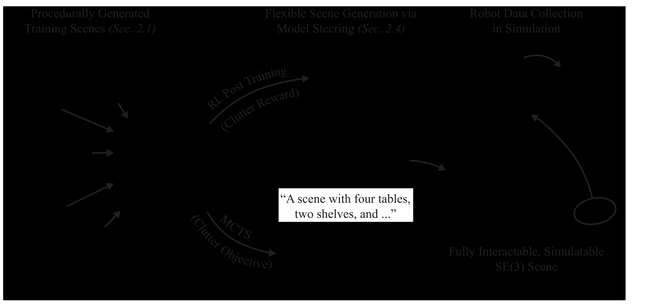
A diffusion model learns which assets to place and their full three-dimensional rigid poses from 44.8 million procedurally generated scenes. The learned scene prior supports reinforcement-learning post training, text or partial-scene conditioning, and inference-time Monte Carlo tree search (MCTS) for goals such as increased clutter.
Projection and simulation repair generated geometry before robot use. Experiments demonstrate generative quality and teleoperated interaction, while large-scale autonomous robot-training benefits remain untested. The project page links code, data and model weights.
1 Introduction
Robotic manipulation needs arrangements of small objects with height, orientation, contact and support relationships. Floor-aligned SE(2) furniture layouts cannot express many such cases. The paper learns an object-set prior over fixed asset identities and SE(3) poses, then steers that prior toward downstream objectives.
Procedural generation supplies broad supervision, while the learned model makes conditional synthesis and adaptation easier. Its 44.8 million arrangements use only 46 unique assets. The central contribution is demonstrating several steering mechanisms on this shared representation, rather than proving that the resulting distribution covers real-world environments.
2 SE(3) Scene Generation and Steering
The pipeline generates procedural training scenes, learns a mixed discrete–continuous diffusion model, and repairs physical violations after sampling. Reinforcement learning, conditioning and search provide complementary ways to change the output distribution.
2.1 Data Generation
All reported training data comes from one spatial scene-grammar framework. A scene is a set of asset identities and poses, so the representation could also accept other procedural or reconstructed real-world sources. Those additional data sources are proposed extensions, not part of these experiments.
2.2 SE(3) Scene Diffusion
Each of at most N object slots contains a three-dimensional translation, a nine-dimensional rotation representation and a one-hot asset category. An empty category allows variable object counts. Rotations are projected onto SO(3) when sampling.
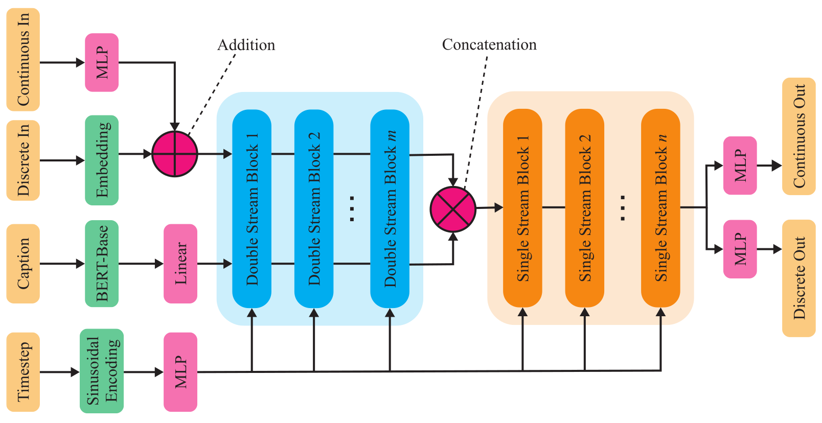
The model combines continuous diffusion for poses with discrete diffusion for categories, conditioning each on the other. A Flux-style transformer omits object positional encodings to preserve permutation equivariance. Separate projections handle discrete and continuous inputs and outputs.
2.3 Physical Feasibility Post Processing
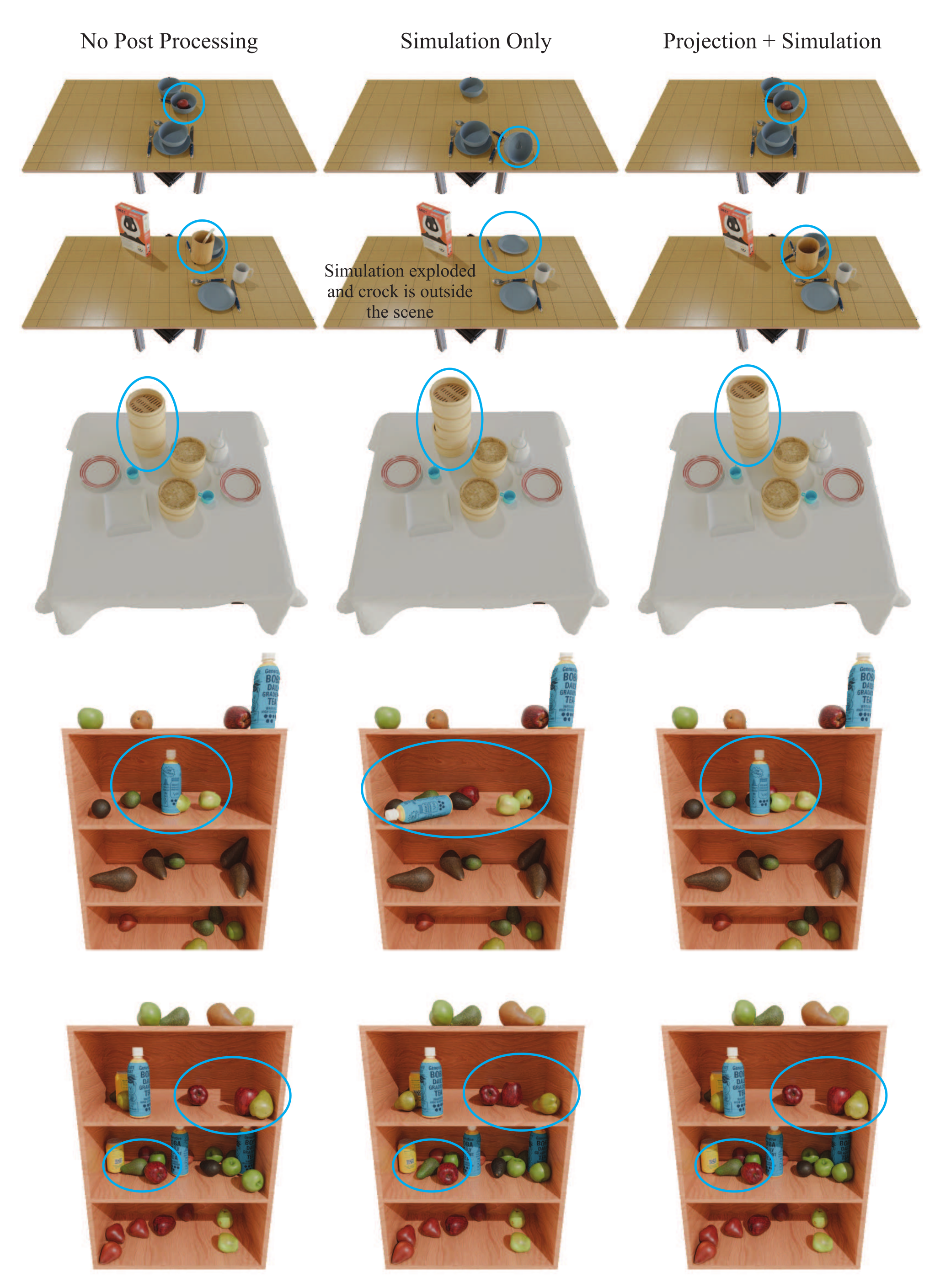
Post processing first moves translations toward a nearby collision-free configuration while fixing orientations. It then simulates the scene in Drake so unsupported or unstable objects can settle. Projection precedes simulation because deep penetrations can otherwise create explosive contact forces.
These steps enforce the intended geometric and stability conditions when they succeed. The nonlinear solver can fail to converge in cluttered scenes, so the method does not provide an unconditional guarantee for every generated sample.
2.4 Steering Scene Generative Models Toward Downstream Objectives
Three steering routes trade additional training, required conditioning data and inference cost. Post training changes model parameters, conditional generation supplies constraints through text or fixed scene components, and MCTS searches over successive inpainting operations.
2.4.1 Post Training with Reinforcement Learning
The reinforcement-learning experiment uses DDPO with a stabilizing diffusion loss and an object-count reward. To use existing training methods, it switches to a fully continuous model in which categories are also continuous. This experiment therefore does not fine-tune the main mixed discrete–continuous model.
2.4.2 Conditional Generation
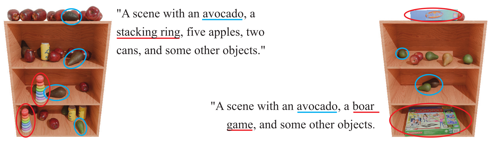
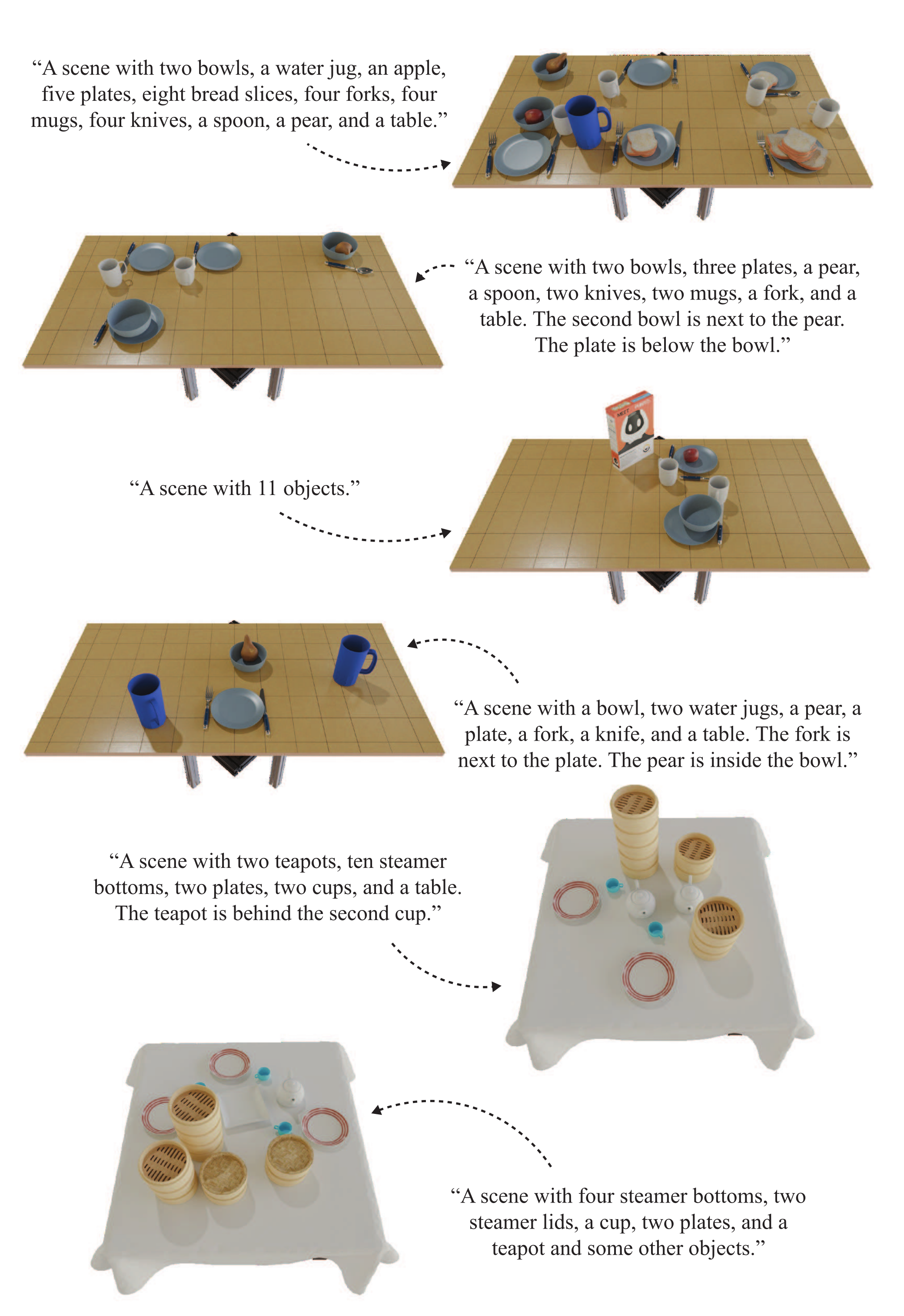
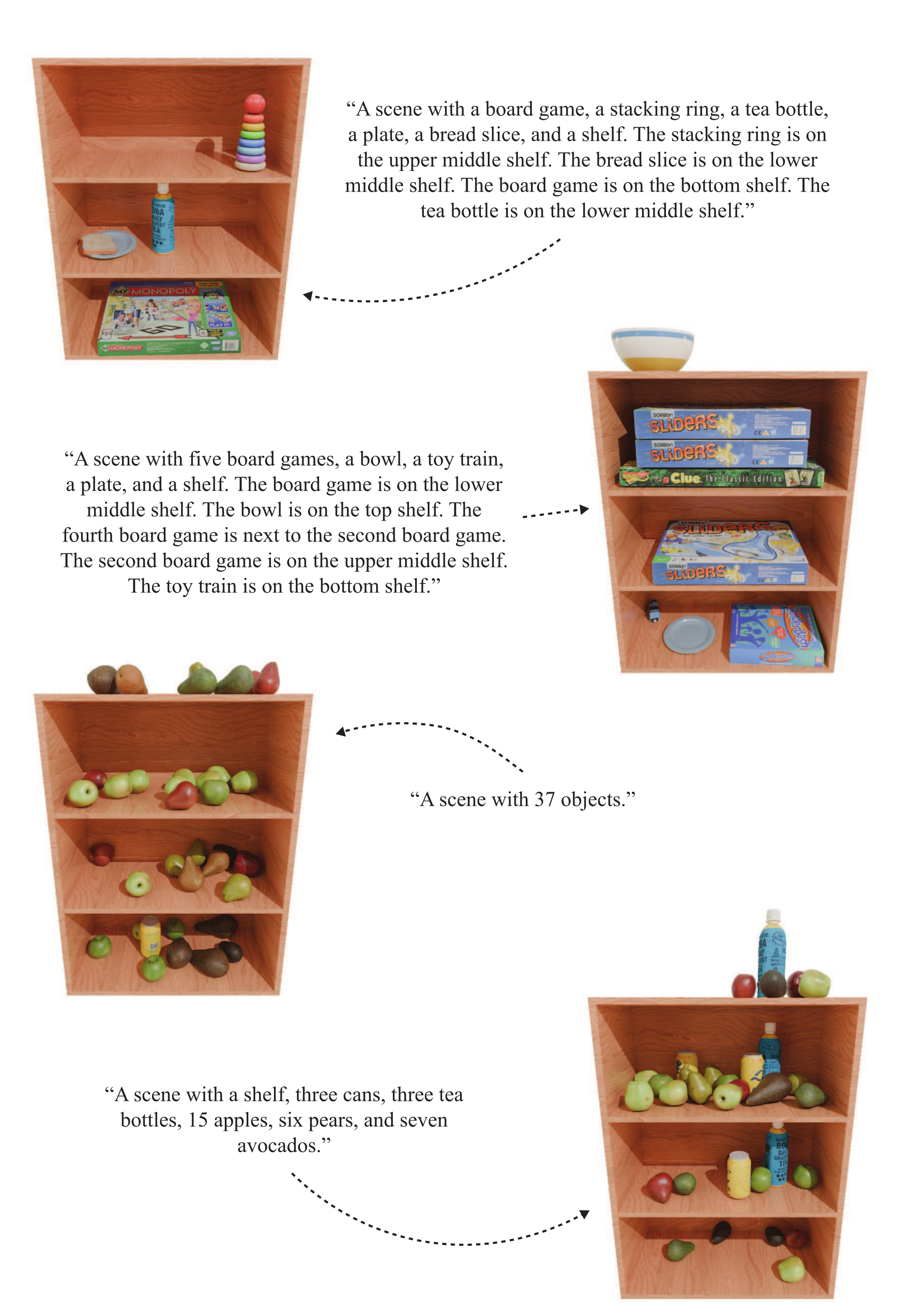
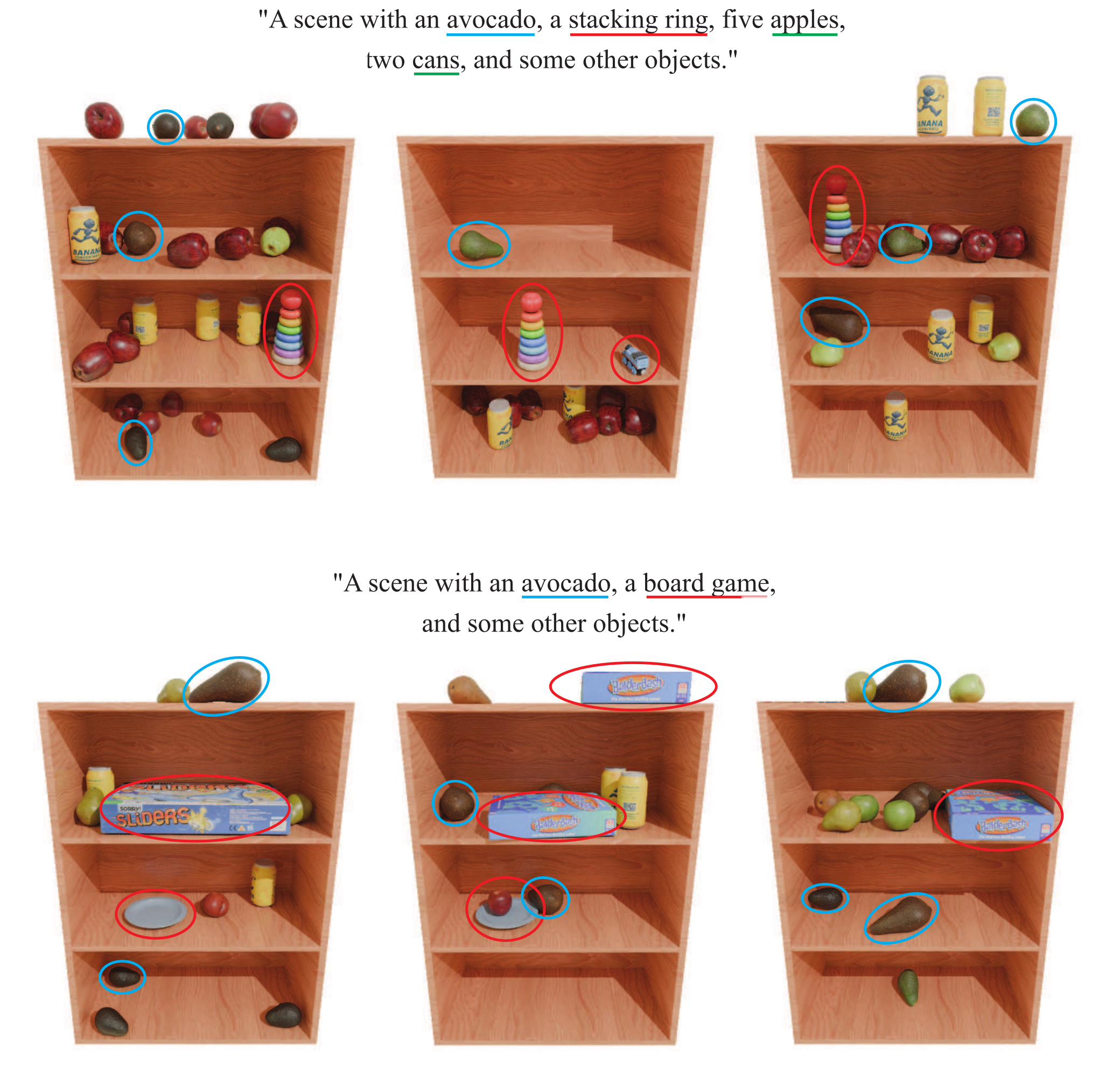
Procedural captions describe counts, object identities or spatial relationships. A frozen BERT encoder supplies text features, and randomly dropping conditioning during training enables classifier-free guidance at inference.
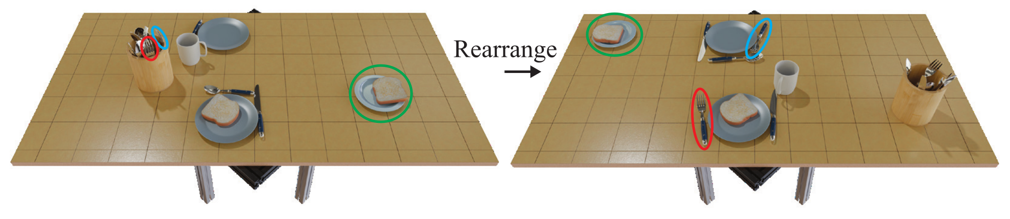
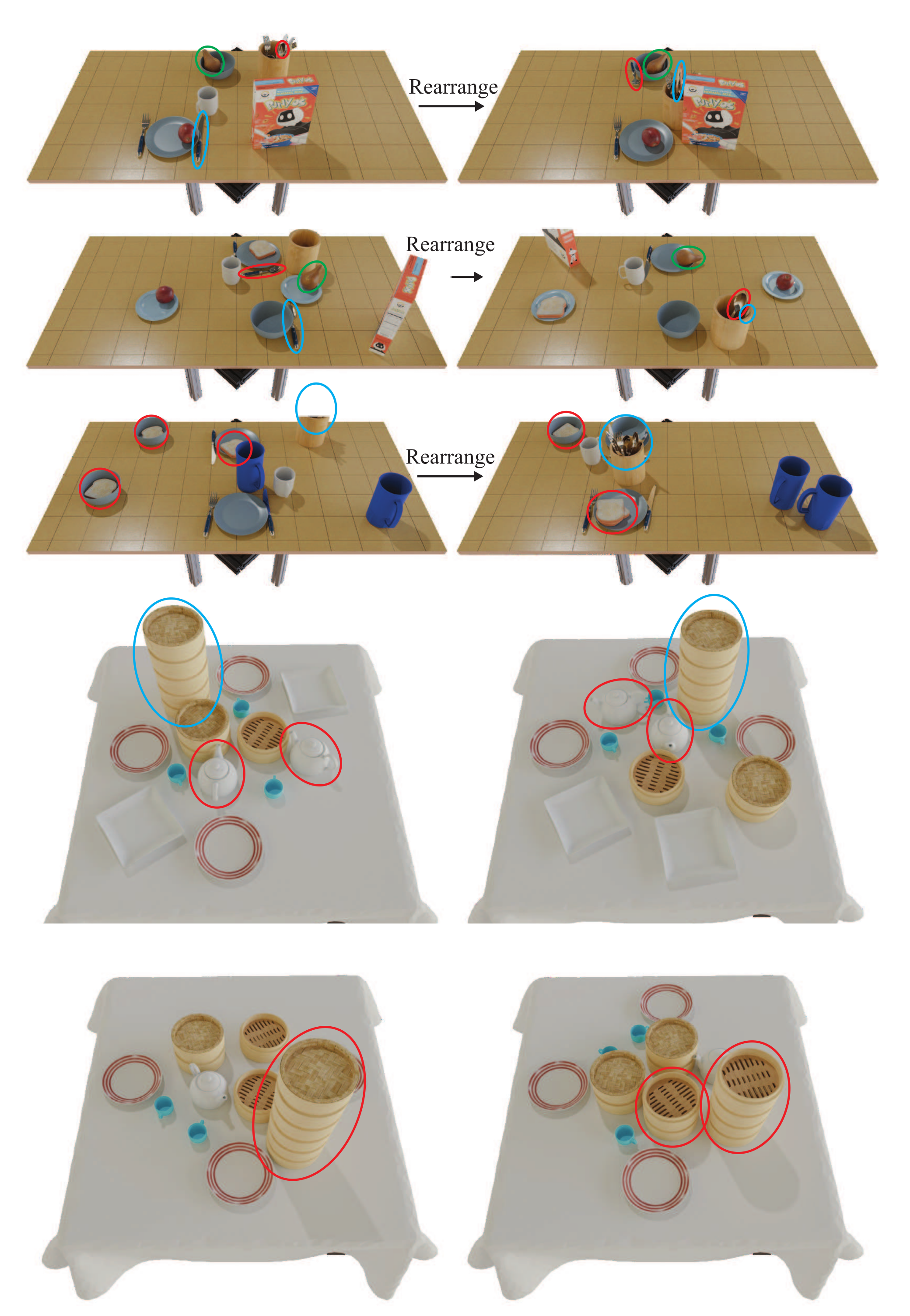
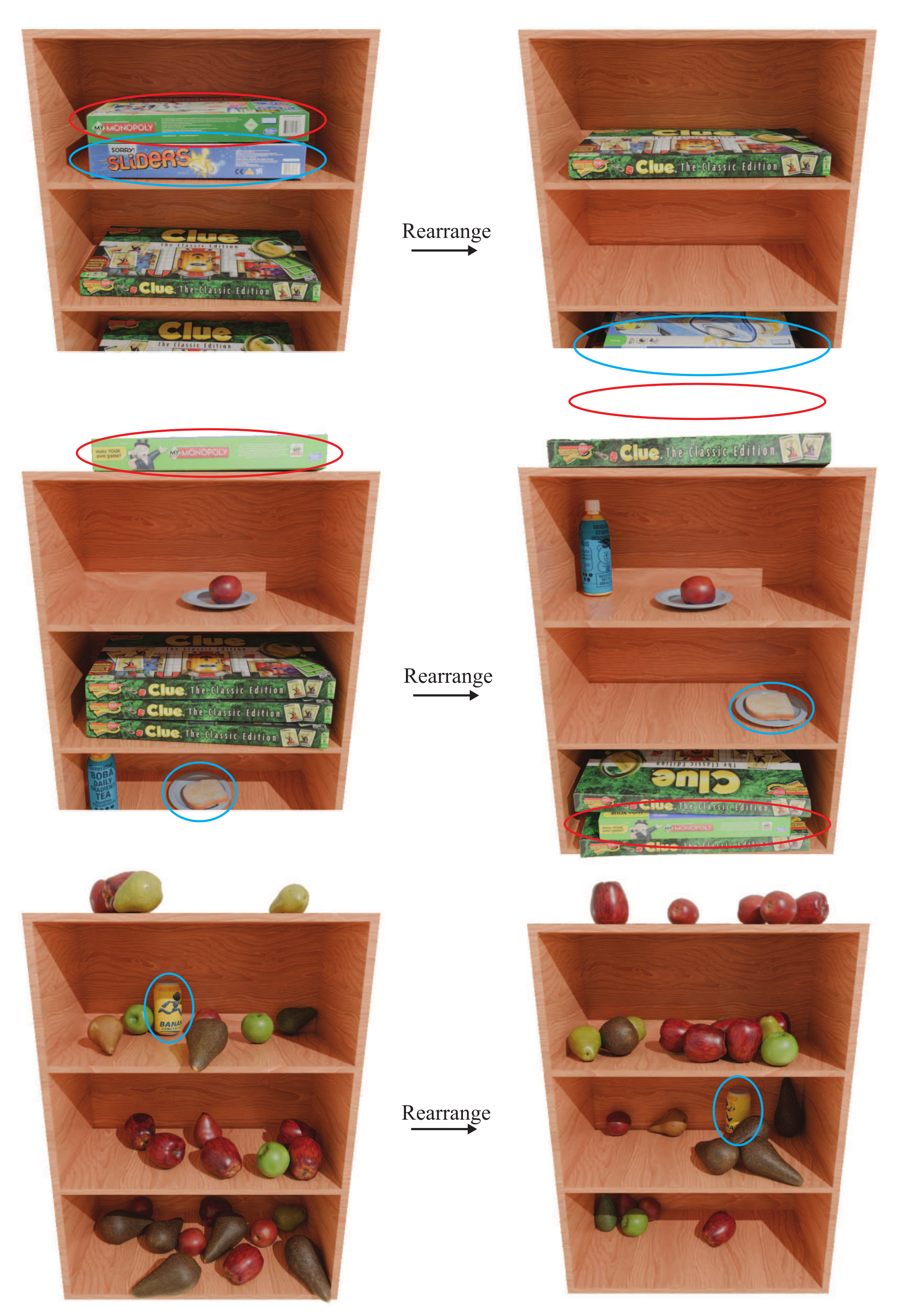
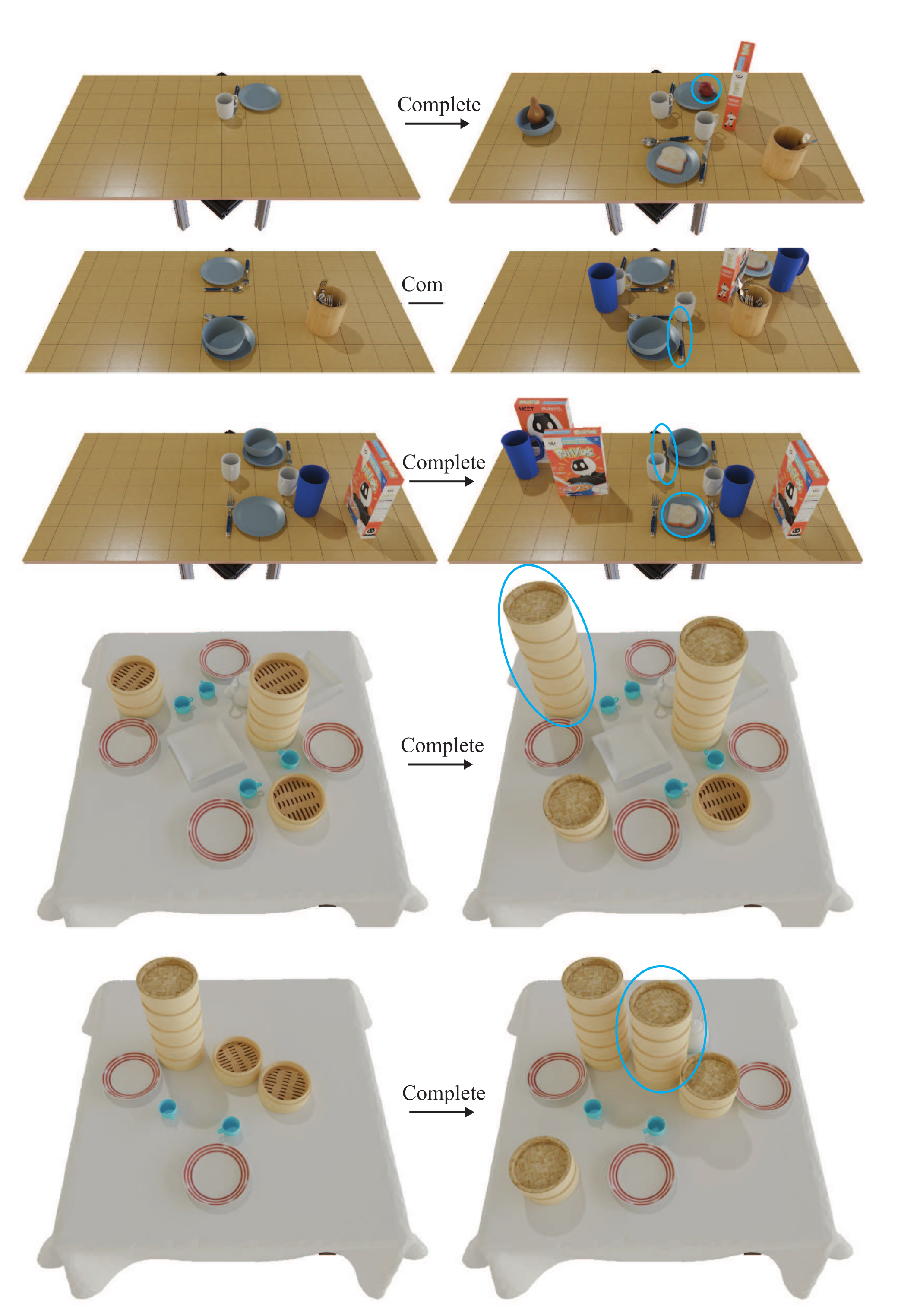
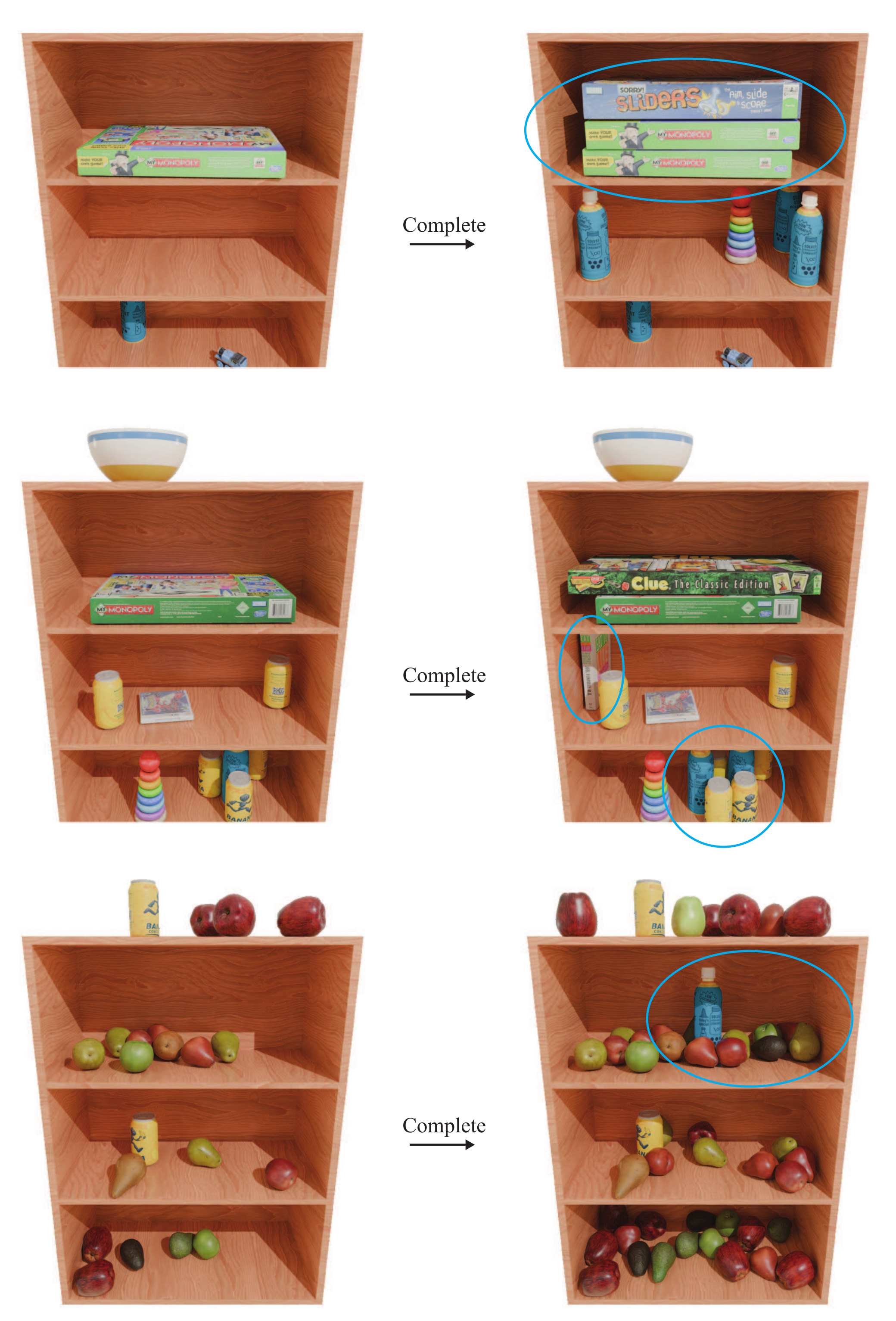
Structured inpainting keeps selected scene components fixed throughout reverse diffusion. Holding categories fixed while resampling poses gives rearrangement; masking empty slots allows completion with new categories and poses. These operations reuse the learned prior rather than constructing a new grammar for each request.
2.4.3 Inference-Time Search via MCTS
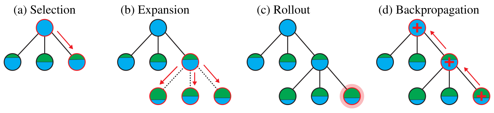
Each MCTS node stores a scene and a mask marking objects to regenerate. Selection balances average reward and exploration with UCT. Expansion samples B inpainted completions using different noise; each completion receives a new invalid-object mask. A randomly selected new child is scored directly, because discarding its masked objects already produces a partial scene, and that reward updates the ancestor statistics.
The reported reward counts physically feasible objects. Search stops at a prescribed iteration budget or when no masked objects remain; otherwise it returns the best partial scene after discarding unresolved objects. The mask generator and reward can differ, allowing other objectives, although such objectives are not evaluated here. The infinite-branching connection to independent random search is conceptual; the main experiment uses B = 3.
Equation
3 Experimental Evaluation
Experiments compare scene-generation metrics against adapted SE(2) baselines and demonstrate the three steering routes. Many steering results are qualitative examples rather than controlled studies of downstream robot-policy performance.
3.1 Evaluation Setup
DiffuScene and MiDiffusion are minimally adapted to the same asset-and-pose representation; all methods use the same BERT text encoder. Five scene types include breakfast tables, dimsum tables, living-room shelves, pantry shelves and restaurants, with low/high clutter variants for breakfast and restaurant scenes.
Evaluation uses semantic-rendering FID and real-versus-generated classifier accuracy (CA), object-category KL divergence, prompt-following accuracy (APF), and pre-repair median total penetration (MTP). CA near 50% means the trained classifier cannot distinguish the rendered distributions; it does not certify physical correctness or full 3D equivalence. Appendix C specifies the viewpoints and sample counts.
3.2 Unconditional Generation
Empty text conditioning supplies unconditional samples. On high-clutter restaurants, the proposed model improves CA to 70.74% and MTP to 6.31 cm, compared with 78.63% and 8.80 cm for MiDiffusion. On living-room shelves, CA is 52.84% and MTP 0.02 cm; FID ties MiDiffusion at 2.09. These penetration values are measured before repair.
Category-frequency KL is not uniformly best. The appendix also contains exceptions to the strongest FID and penetration comparisons, so performance should be read metric by metric.
| Method | Restaurant (High-Clutter Variant) | Living Room Shelf | ||||||
|---|---|---|---|---|---|---|---|---|
| CA (50 it, %) | KL () | FID | MTP (cm) | CA (100 it, %) | KL () | FID | MTP (cm) | |
| DiffuScene* [30] | 84.81 ± 6.49 | 0.55 | 1.39 | 18.11 | 71.73 ± 0.99 | 4.67 | 2.18 | 0.05 |
| MiDiffusion* [31] | 78.63 ± 9.79 | 1.01 | 1.34 | 8.80 | 64.13 ± 1.87 | 2.51 | 2.09 | 0.03 |
| Ours | 70.74 ± 8.05 | 0.87 | 1.31 | 6.31 | 52.84 ± 1.26 | 2.13 | 2.09 | 0.02 |
3.3 Post Training with Reinforcement Learning
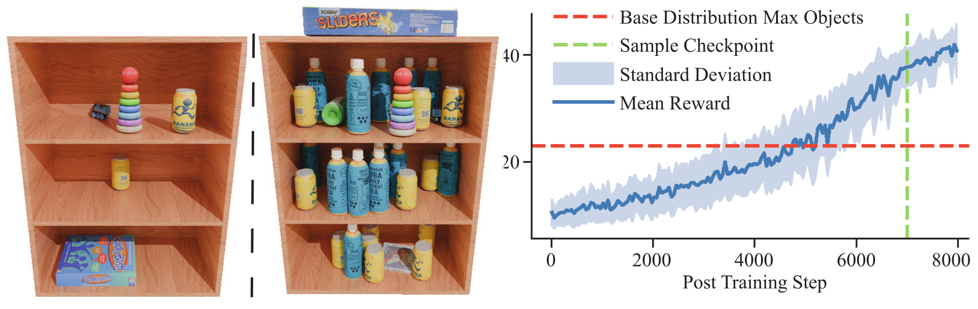
Object-count post training increases shelf clutter beyond the largest count seen during pretraining. The representation’s capacity is enlarged by 20 slots before fine-tuning. Figure 4 marks the training maximum of 23 objects and a checkpoint at step 7000 selected before excessive optimization harms appearance.
Increasing the reward can produce many objects while weakening resemblance to the source distribution. The experiment demonstrates a controllable distribution shift, not monotonic improvement in all aspects of scene quality.
3.4 Conditional Generation
Table 2 reports stronger CA, FID and count/category prompt adherence on high-clutter breakfast scenes and pantry shelves. APF reaches 0.86 and 0.98 respectively, versus 0.76 and 0.88 for DiffuScene. APF does not evaluate the full spatial-language content of the captions.
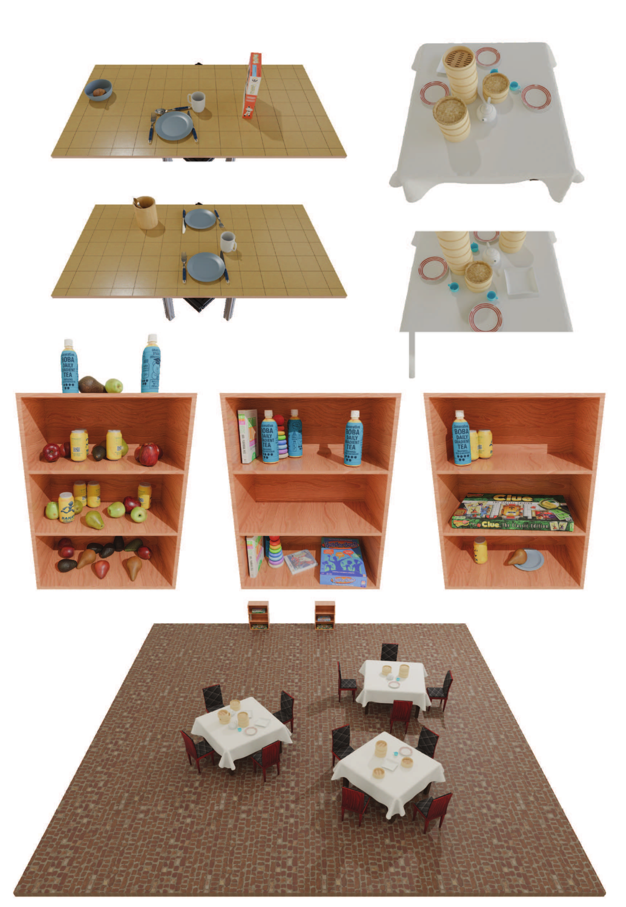
Rearrangement examples keep identities while changing full rigid poses, including cutlery orientation. A model trained on equal mixtures of living-room and pantry shelves generates combinations containing assets from both sets. These are qualitative demonstrations of compositional conditioning within a shared asset library.
| Method | Breakfast Table (High-Clutter Variant) | Pantry Shelf | ||||||
|---|---|---|---|---|---|---|---|---|
| CA (50 it, %) | KL () | FID | APF | CA (50 it, %) | KL () | FID | APF | |
| DiffuScene* [30] | 82.38 ± 3.82 | 0.96 | 1.87 | 0.76 | 84.65 ± 2.23 | 0.91 | 1.93 | 0.88 |
| MiDiffusion* [31] | 82.22 ± 3.11 | 0.58 | 1.93 | 0.60 | 87.24 ± 1.80 | 0.64 | 1.89 | 0.72 |
| Ours | 68.44 ± 4.67 | 0.30 | 1.84 | 0.86 | 82.78 ± 3.44 | 0.66 | 1.88 | 0.98 |
3.5 Inference-Time Search
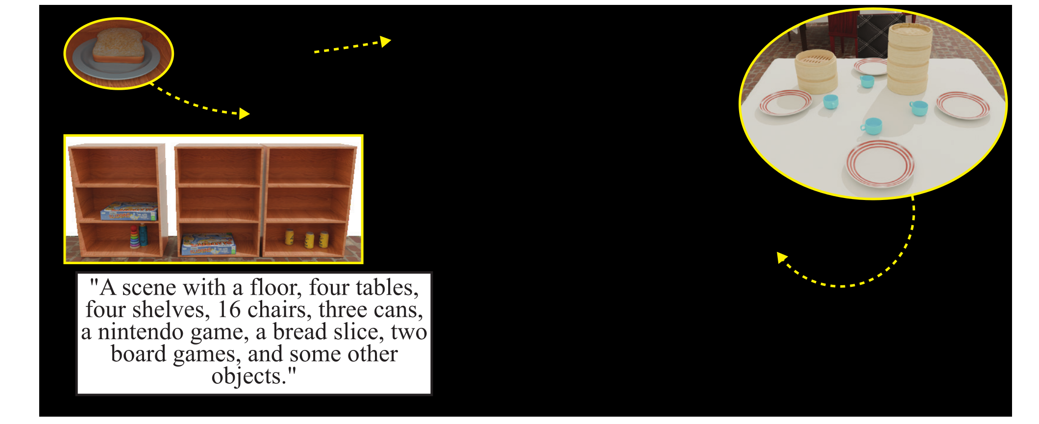
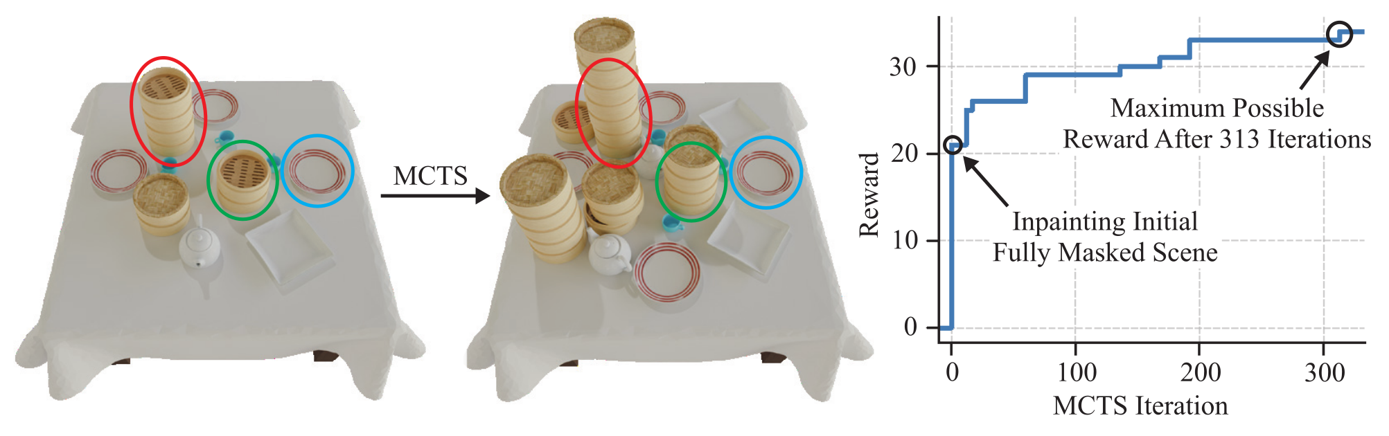
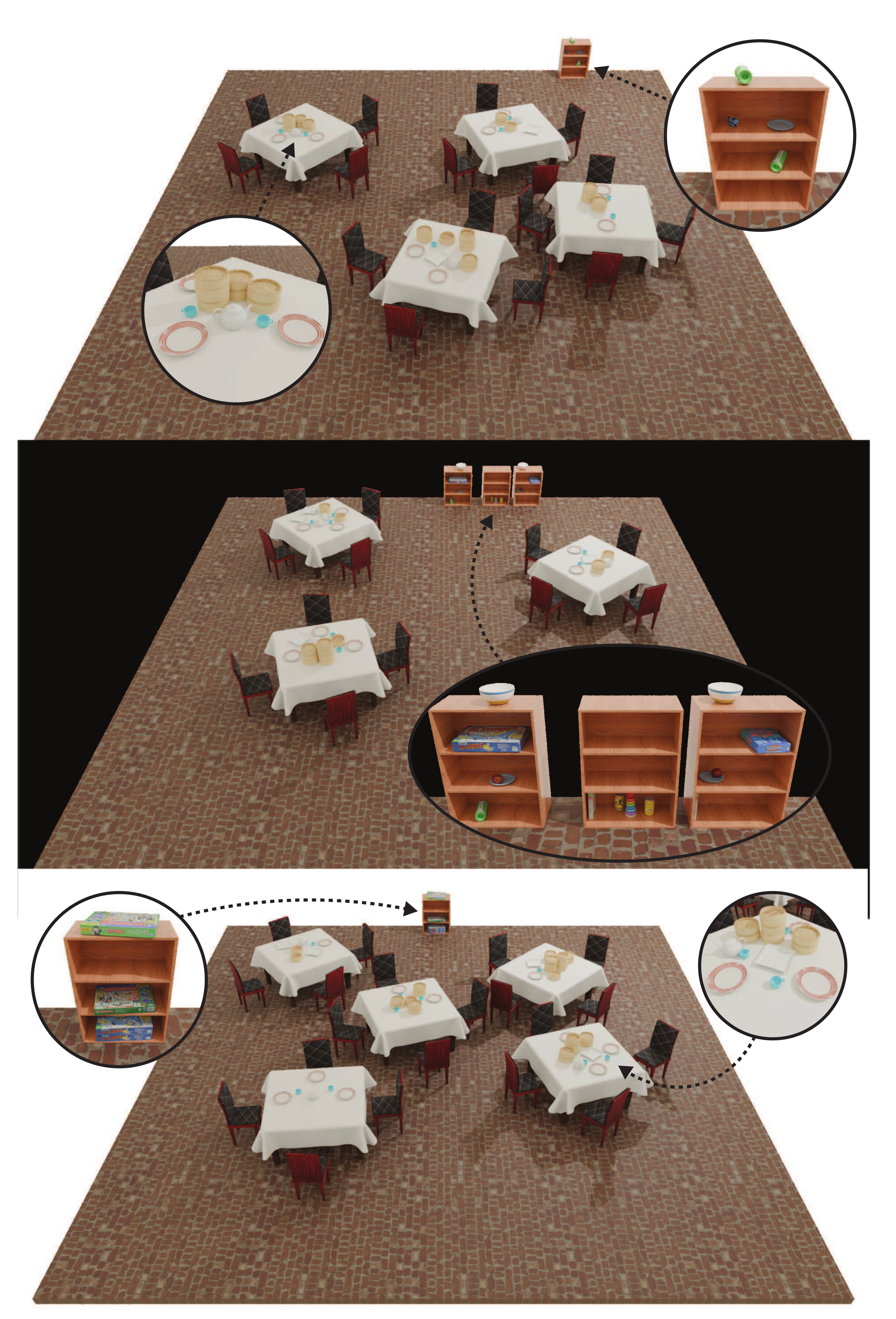
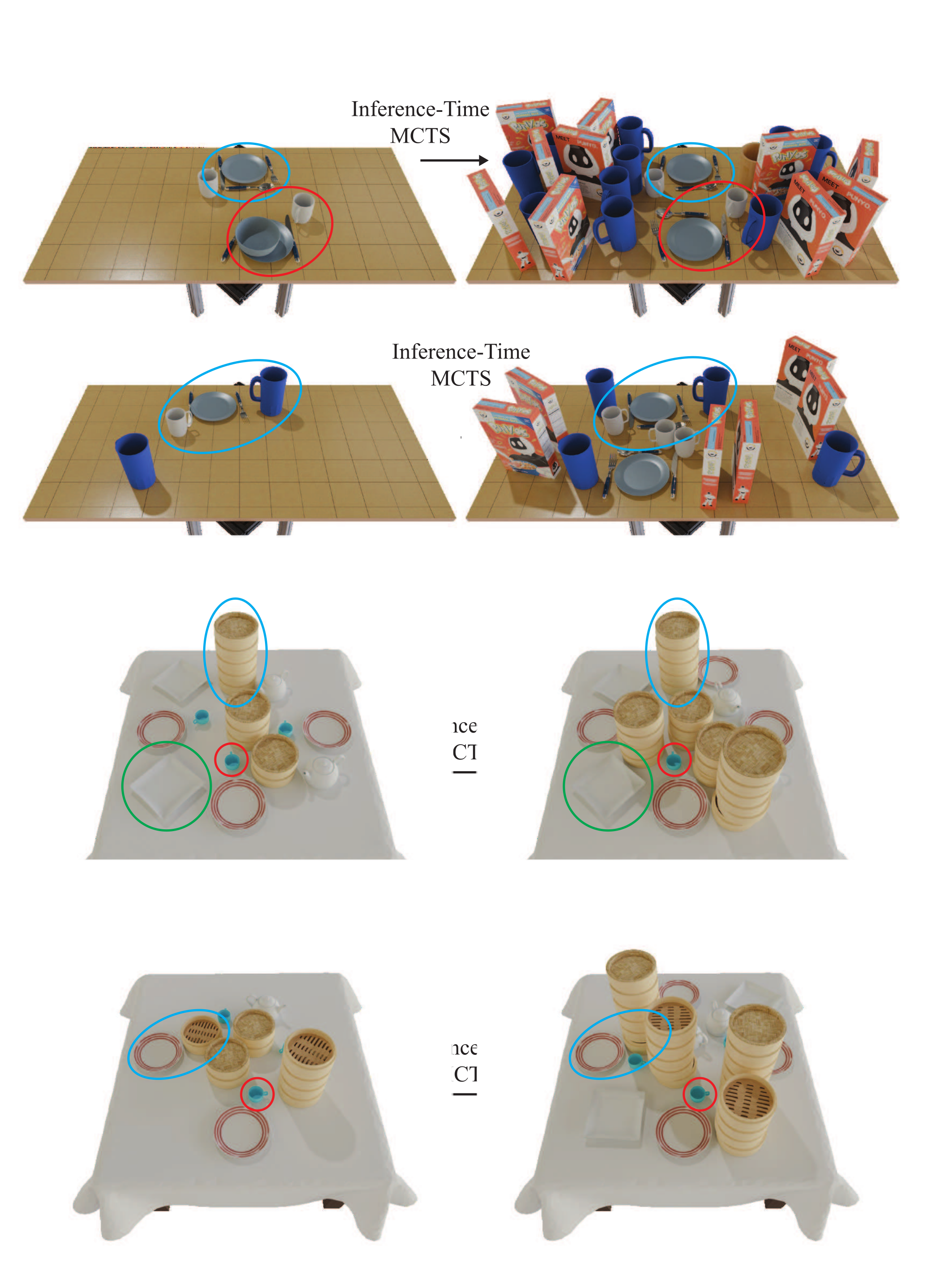
With branching factor three, the illustrated dimsum search improves from 21 feasible objects among the best three initial samples to 34 after 313 iterations. Thirty-four is the training-set maximum, so this example exceeds typical counts rather than the observed maximum. The main text gives a mean of 17.1; the dataset table instead reports 18.14 for dimsum.
The search builds on learned structure such as steamer stacks. The paper does not provide an equal-compute benchmark against other search algorithms or a broad distribution of search success and runtime.
4 Conclusion
The learned prior supports several routes from procedural data to task-directed scenes. Generated scenes were imported into Drake and used for teleoperated pick-and-place with a mobile KUKA iiwa without manual scene correction in the shown subset. This supports practical simulation use, while autonomous training gains and deployment at scale remain future work.
5 Limitations
The procedural distribution and fixed library limit environmental realism and novel-geometry generalization. The evaluated assets are rigid; articulated scenes are proposed but not demonstrated. Reinforcement learning is tested only on a continuous variant and a count reward, and excessive optimization or too many additional slots can damage sample quality.
Conditioning, post training and search are proof-of-concept adaptation studies. More realistic data, richer rewards and large-scale autonomous robot training are open directions. Physical projection can fail, and the visual metrics and short stability tests provide limited evidence about all aspects of a generated scene.
Acknowledgments
Amazon and the Toyota Research Institute partially supported the work. The authors state that the conclusions represent their views rather than those of Toyota entities and acknowledge colleagues for discussion.
Appendix A Procedurally Generated Datasets
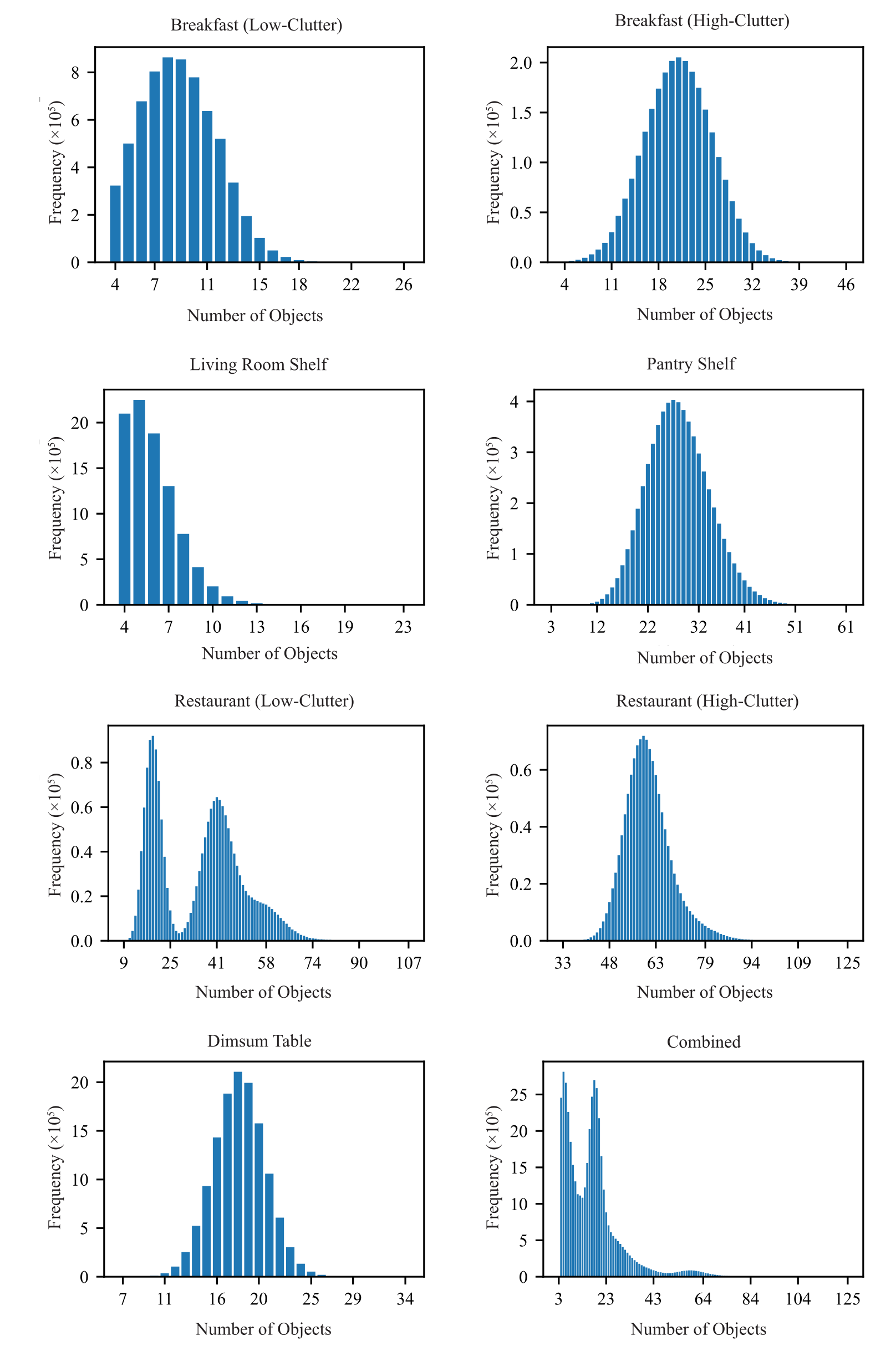
The dataset contains 44,790,942 distinct arrangements with three to 125 objects, drawn from 46 assets across five scene types and seven listed variants. Dimsum accounts for more than 13 million scenes. This scale comes from combinatorial arrangements of a small library, rather than a comparable expansion in object geometry diversity.
Table 3 and Figure 8 retain every dataset count and object-count distribution. Some distributions have long tails; equal dataset mixing during training differs from sampling proportionally to these raw scene totals.
| Dataset | # Object | Min | Max | Mean | Total |
|---|---|---|---|---|---|
| Assets | Objects | Objects | Objects | Scenes | |
| Breakfast Table (Low-Clutter) | 14 | 4 | 26 | 8.87 | 6,679,981 |
| Breakfast Table (High-Clutter) | 15 | 4 | 46 | 20.96 | 2,655,407 |
| Dimsum Table | 7 | 7 | 34 | 18.14 | 13,042,071 |
| Living Room Shelf | 18 | 4 | 23 | 5.93 | 9,087,513 |
| Pantry Shelf | 14 | 3 | 61 | 27.98 | 6,171,940 |
| Restaurant (High-Clutter) | 27 | 33 | 125 | 60.54 | 1,195,751 |
| Restaurant (Low-Clutter) | 27 | 9 | 107 | 35.08 | 1,797,170 |
| All Datasets Combined | 46 | 3 | 125 | 17.17 | 44,790,942 |
A.1 Procedural Data Generation
Probabilistic context-free grammars recursively spawn objects and sample their poses. Cross-branch constraints such as collisions require rejection sampling and Hamiltonian Monte Carlo beyond the grammar itself. A separate grammar is implemented for each scene type.
Generation runs across 192 CPUs on AWS M7A Metal instances. The hardest reported setting yields about 60,000 valid scenes per instance per day because many proposals violate constraints. The learned model is intended to amortize this expensive procedure, although the paper does not report a full throughput comparison for every setting.
A.2 Text Prompt Generation
A rule-based captioner describes total count, object names and position-derived relations. It can list all assets or a subset, preferentially mention large furniture in room scenes, and use ordinal names to distinguish repeated categories. Spatial relations are limited to named nearby objects and scene-specific shelf or room rules.
Each scene is duplicated three times for annotation purposes, with a different annotation type for each copy. These captioned copies do not represent additional unique physical scenes.
Appendix B Implementation Details
The implementation appendix specifies architecture, training, physical repair, steering procedures and their computational tradeoffs. The released implementation provides the complete codebase.
B.1 Model Architecture
Discrete and continuous scene tokens are embedded separately and added. Double-stream transformer blocks process text and scene features with separate weights, merging them for attention; single-stream blocks operate after token concatenation. Output MLPs decode the discrete and continuous components.
The text encoder is frozen BERT-Base. Sinusoidal timestep embeddings enter modulation layers, and the scene stream has no positional encoding so object ordering does not change the modeled set.
B.2 Model Training
The 88.3-million-parameter model has five double-stream and ten single-stream blocks. Training uses AdamW at 2×10⁻⁴ learning rate and 10⁻³ weight decay, cosine decay, 5,000 warmup iterations, EMA updates and 1,000 diffusion steps. Conditioning is dropped with 10% probability; text inputs contain up to 110 tokens.
Runs use 200,000 iterations, batch size 256 per GPU and eight A100 GPUs. Final models use full precision, with 80 GB devices for restaurants and cotraining. Reported training time ranges from 1.06 days for dimsum to 1.65 days for full cotraining. Low-precision development is faster but can compromise fine positional accuracy.
B.3 Cotraining Recipe
Cotraining selects subdatasets uniformly rather than in proportion to their scene counts. Each has an infinite iterable stream with random offsets and buffered shuffling. The same balancing principle is used for the two shelf datasets and for the combined scene collection.
B.4 Physical Feasibility Post Processing
The retained optimization minimizes squared translation changes subject to nonnegative signed distances between objects, while keeping orientations fixed. SNOPT solves the nonlinear program before simulation adjusts full poses.
Complex contact configurations, nonconvexity and tight tolerances can prevent convergence, especially for restaurants. The source’s broader claims of guaranteed zero penetration should be understood as the constraint target when projection succeeds. Figure 34 illustrates selected successes rather than an overall solver-success rate.
Equation 1
| (1) |
B.5 Post Training with Reinforcement Learning
DDPO uses a score-function/REINFORCE estimator without a learned value function or importance sampling. DDIM produces 100–150-step trajectories; gradients cover all timesteps or a sampled subset. The same scheduler and step count are used at training and inference, since mismatches reduce the observed improvement.
Rewards are measured only on the final scene and consist of object count. Batch-normalized advantages use globally synchronized statistics across workers. A DDPM auxiliary loss, weighted by a coefficient in the tested range 100–200, stabilizes optimization. Fine-tuning uses batch size 32 per GPU on eight A100 80 GB devices.
Extending this objective to discrete and mixed diffusion is discussed but not evaluated. Practical few-step discrete samplers are identified as a remaining obstacle.
Equation 2
| (2) |
B.6 Conditional Generation
Conditioning can be supplied through text features learned during training or through fixed scene components during inpainting. These mechanisms share the scene representation but impose different requirements on training data.
B.6.1 Text-Conditioned Generation
The retained guidance equation combines conditional and unconditional predictions for both pose and category components. Under the paper’s convention, weight −1 gives unconditional sampling, zero gives ordinary conditional sampling, and positive weights strengthen guidance. A frozen BERT-Base encoder supplies up to 110 prompt tokens.
Equation 3
| (3) |
B.6.2 Inpainting
Masked attributes begin from noise and evolve through reverse diffusion; unmasked components remain clamped to their original values. The mask can target complete objects, just poses, or empty slots, supporting rearrangement and completion without retraining.
B.7 Inference-Time Search via MCTS
Search repeatedly resamples masked portions and evaluates completed partial scenes. The implemented objective counts feasible objects, although the interfaces allow separate choices of a mask generator and reward.
B.7.1 Mask Generator
Drake’s signed-distance checker identifies penetrating pairs, and every object in such a pair is masked. Stability is approximated by 0.1 seconds of simulation: translations or rotations exceeding thresholds mark an object unstable. Penetrating objects are removed before that simulation to avoid misleading contacts.
Predefined welded supports such as tables and shelves are never masked. This preserves the base on which other objects depend. The finite simulation horizon and unspecified thresholds make this an operational feasibility test, not a proof of long-term stability.
B.7.2 Reward Function
Each nonpenetrating, sufficiently stable object contributes one unit of reward. This binary count favors increasing the number of accepted objects; it does not directly measure diversity, visual realism, robot reachability or manipulation difficulty.
B.7.3 Relation to Gradient-Based Guidance
Gradient-based guidance is an alternative when the reward is differentiable and can be cheaper. MCTS accepts nondifferentiable objectives, including simulator-based checks, at the expense of repeated generation and evaluation. No direct guidance-versus-search benchmark is supplied.
B.8 Comparison of Steering Methods
Post training requires optimization but keeps inference fast. Text conditioning requires labeled training examples, while inpainting reuses an existing model without new training. MCTS offers flexible objectives without parameter updates but makes inference slower. Combining these strategies is possible; the paper does not evaluate every proposed combination.
Appendix C Metric Definitions and Evaluation Details
Metrics use 5,000 training scenes and 5,000 generated scenes. Conditional prompts are taken from the training scenes. Semantic renders use one manually chosen viewpoint per scene type at 640×480 resolution; occlusion means these image-based scores cannot inspect the complete 3D state.
CA is averaged across ten train/test splits, with classifier training length tuned by dataset and held fixed across methods. FID compares rendered features; KL compares category frequencies. APF checks counts and category inclusion, not spatial relations. MTP is defined here as median total penetration before repair, although later prose sometimes calls it a mean. Claimed zero post-projection penetration remains conditional on a successful solve.
Appendix D Additional Results
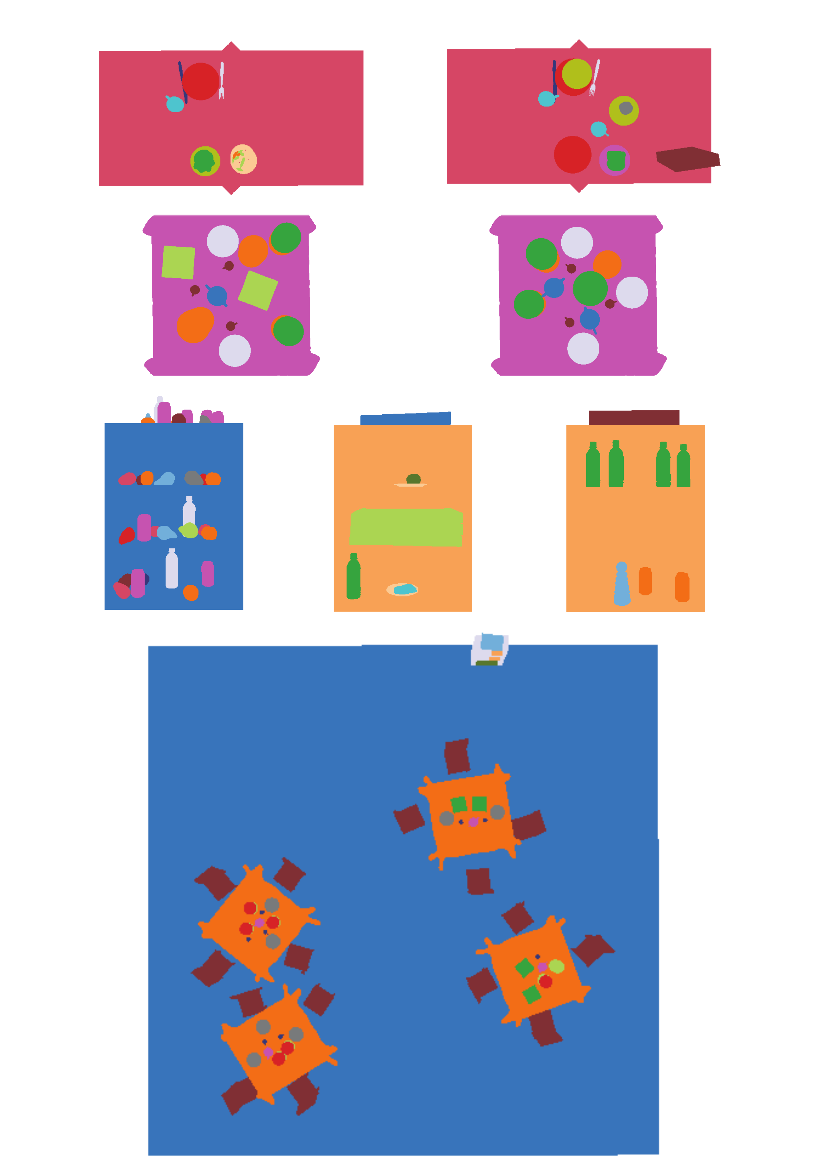
The full galleries and tables retain unconditional samples, post-trained outputs, conditional generation, rearrangement, completion, search trajectories and nearest-neighbor comparisons. They complement the main experiments without constituting additional autonomous robot-training evaluations.
D.1 Unconditional Generation
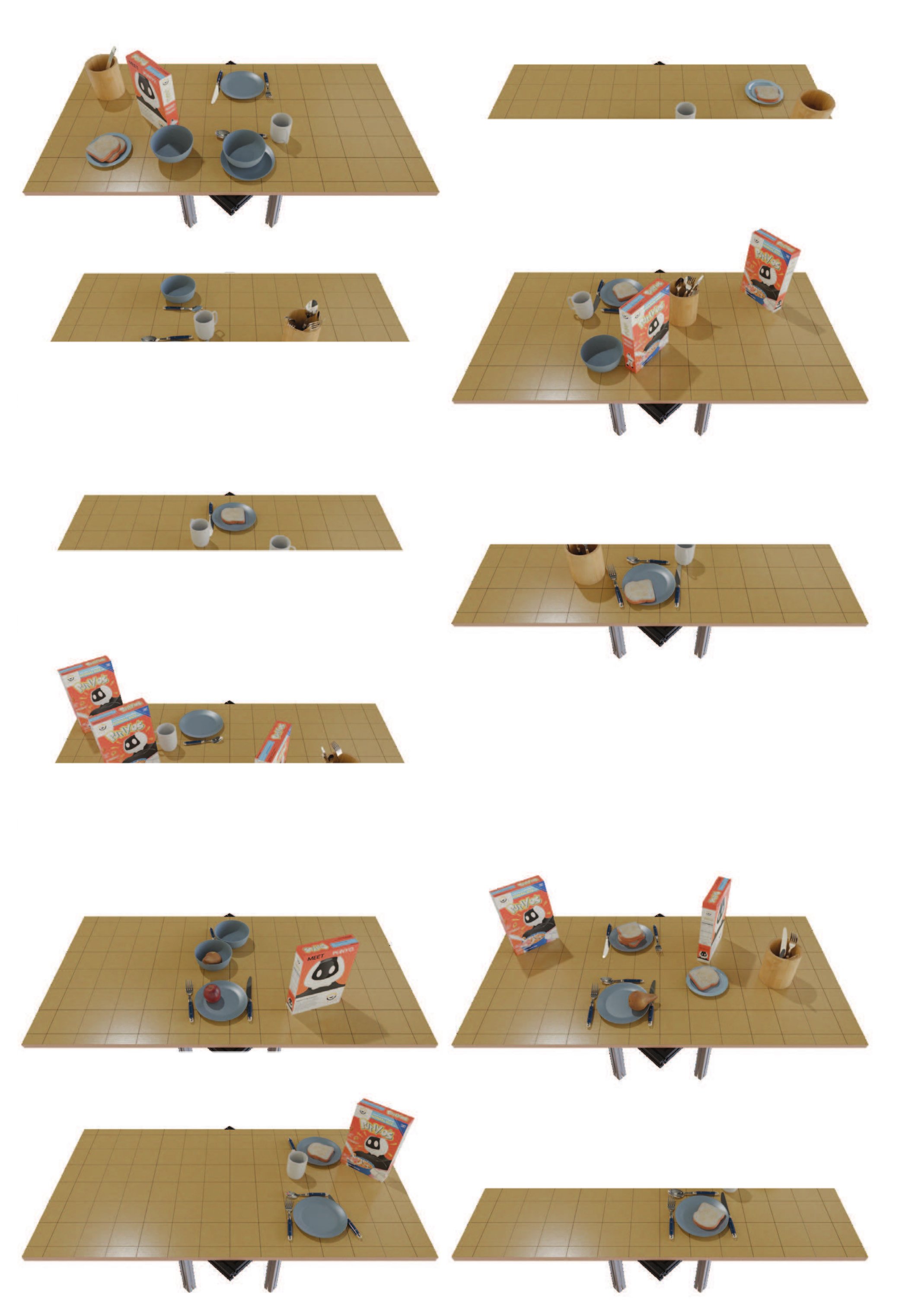
Tables 4–6 extend unconditional comparisons across all datasets. CA is lowest for the proposed model throughout, but FID is slightly worse than DiffuScene for high-clutter breakfast scenes (1.88 versus 1.86). Dimsum penetration is also slightly higher (0.20 versus 0.18 cm), and high-clutter breakfast penetration ties at 6.97 cm.
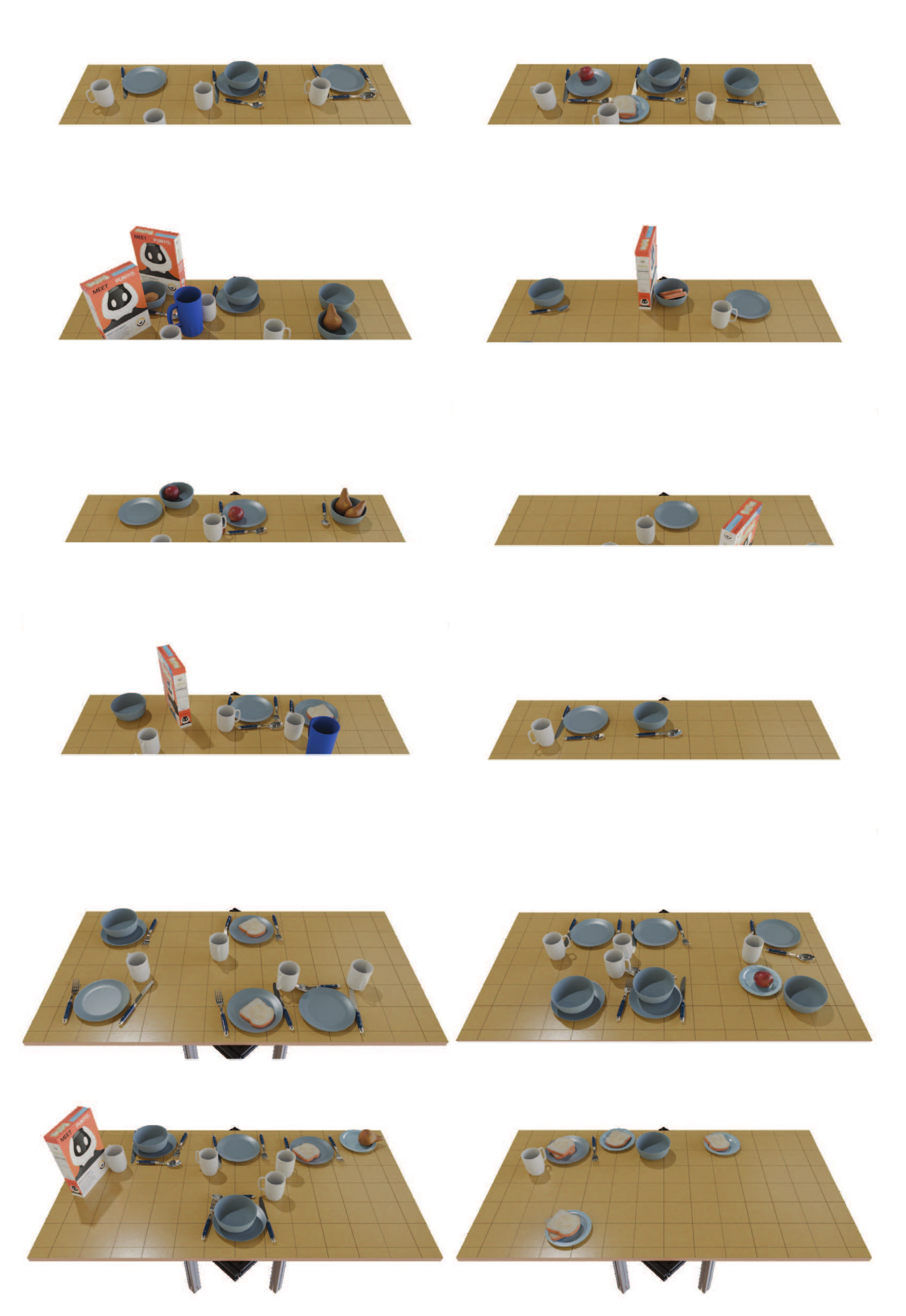
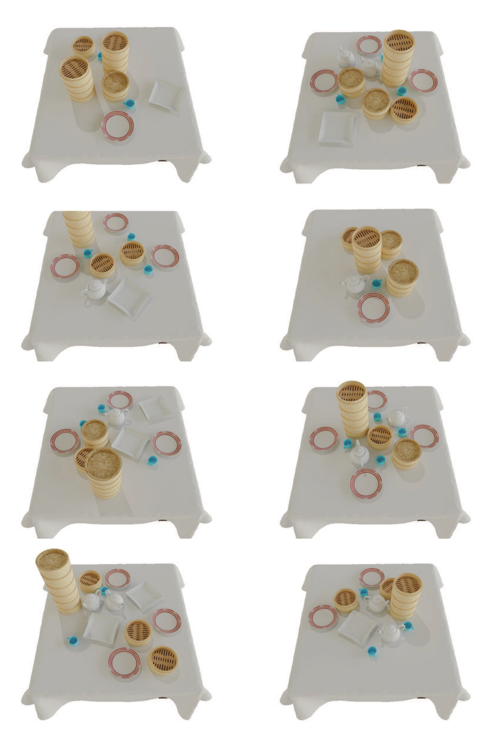
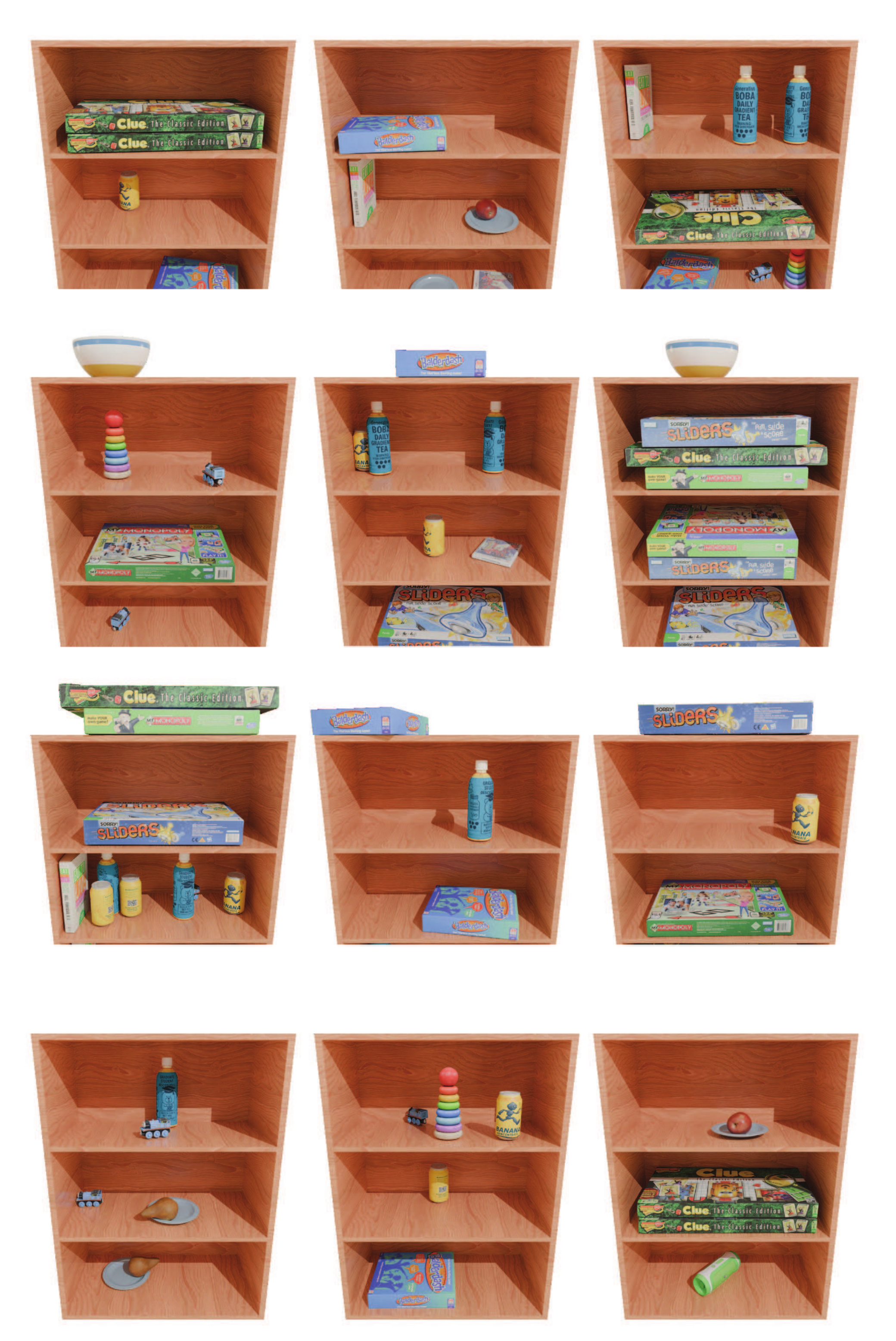
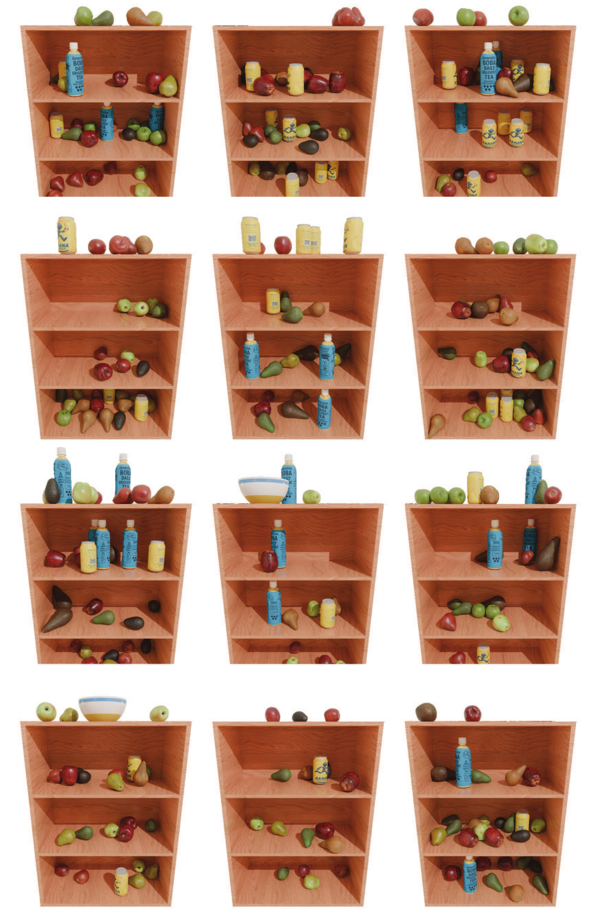
Figures 11–17 show every per-dataset gallery and the jointly trained model. These reveal the range of sampled arrangements within the asset library; category KL and geometric metrics remain separate from visual distribution matching.
| Method | Pantry Shelf | Breakfast Table (Low-Clutter Variant) | ||||||
|---|---|---|---|---|---|---|---|---|
| CA (50 it, %) | KL () | FID | MTP (cm) | CA (25 it, %) | KL () | FID | MTP (cm) | |
| DiffuScene* [30] | 84.38 ± 1.79 | 1.99 | 1.97 | 9.32 | 68.32 ± 8.48 | 2.64 | 2.59 | 5.94 |
| MiDiffusion* [31] | 85.42 ± 0.98 | 1.18 | 1.90 | 5.57 | 65.34 ± 7.39 | 1.79 | 2.43 | 3.81 |
| Ours | 84.04 ± 0.58 | 1.45 | 1.89 | 4.92 | 57.85 ± 4.98 | 1.67 | 2.39 | 3.50 |
| Method | Dimsum Table | Breakfast Table (High-Clutter Variant) | ||||||
|---|---|---|---|---|---|---|---|---|
| CA (100 it, %) | KL () | FID | MTP (cm) | CA (50 it, %) | KL () | FID | MTP (cm) | |
| DiffuScene* [30] | 83.56 ± 8.14 | 0.39 | 0.95 | 0.18 | 81.71 ± 5.00 | 1.57 | 1.86 | 6.97 |
| MiDiffusion* [31] | 78.69 ± 10.25 | 0.57 | 0.96 | 0.19 | 78.86 ± 4.89 | 0.84 | 1.943 | 7.31 |
| Ours | 57.66 ± 4.70 | 0.63 | 0.89 | 0.20 | 69.82 ± 5.37 | 0.81 | 1.88 | 6.97 |
D.2 Post Training with Reinforcement Learning
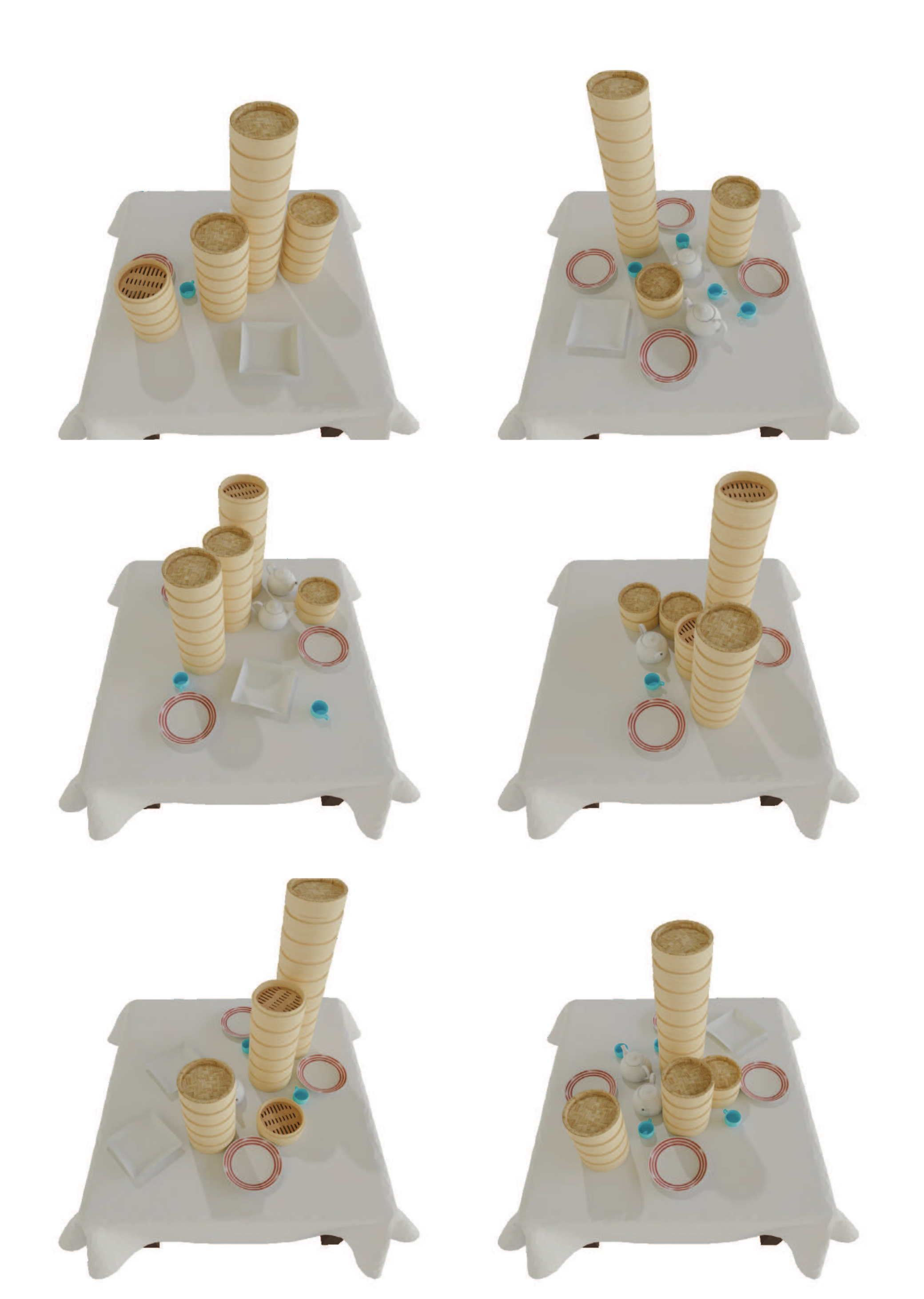
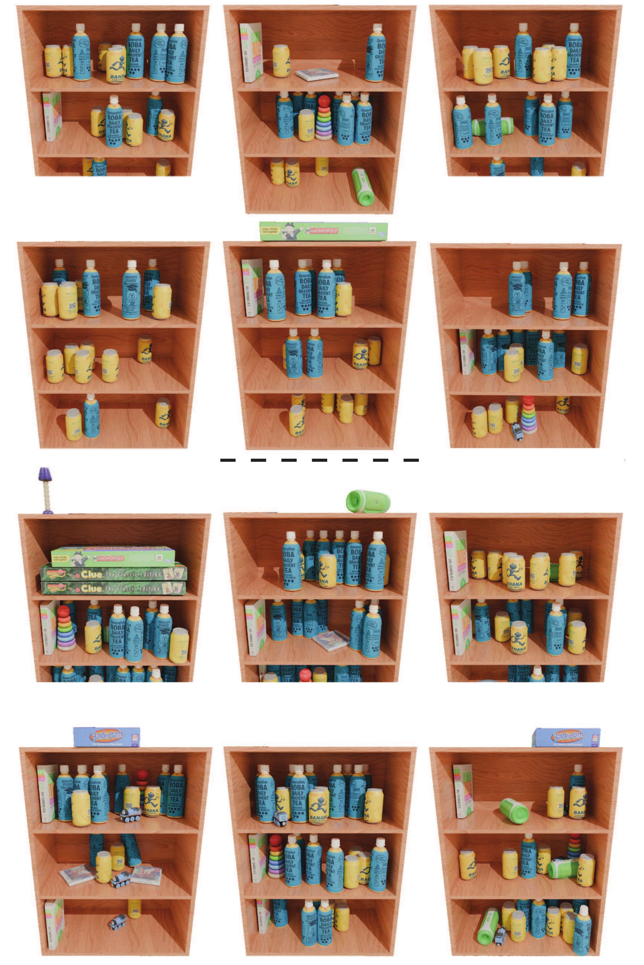
Post-trained dimsum scenes contain taller steamer stacks, while shelf samples become denser. Figure 19 separates outputs with the original slot capacity from those with 20 extra slots. The examples illustrate how a count reward changes a prior; they do not establish improvements on every quality metric.
D.3 Conditional Generation
Tables 7–9 show stronger conditional CA and best-or-tied FID/APF across the tested datasets. APF ties DiffuScene on dimsum (0.90) and living-room shelves (0.99), so the results are not strict wins in every cell. CA measures distribution distinguishability rather than whether each individual prompt is obeyed.
Figures 20–28 retain all prompted samples, pose rearrangements, completions and shelf-mixture examples. Rearrangement keeps identities fixed; completion keeps the unmasked scene fixed. The shelf interpolation examples use guidance weight five and combine assets from both training distributions.
| Method | Dimsum Table | Breakfast Table (Low-Clutter Variant) | ||||||
|---|---|---|---|---|---|---|---|---|
| CA (100 it, %) | KL () | FID | APF | CA (25 it, %) | KL () | FID | APF | |
| DiffuScene* [30] | 87.64 ± 6.34 | 0.22 | 0.94 | 0.90 | 69.13 ± 8.71 | 3.12 | 2.62 | 0.83 |
| MiDiffusion* [31] | 79.26 ± 10.48 | 0.08 | 0.92 | 0.84 | 67.91 ± 8.29 | 1.78 | 2.53 | 0.77 |
| Ours | 60.85 ± 6.52 | 0.18 | 0.89 | 0.90 | 58.46 ± 5.35 | 1.34 | 2.42 | 0.87 |
| Method | Living Room Shelf | Restaurant (High-Clutter Variant) | ||||||
|---|---|---|---|---|---|---|---|---|
| CA (100 it, %) | KL () | FID | APF | CA (50 it, %) | KL () | FID | APF | |
| DiffuScene* [30] | 69.33 ± 1.35 | 3.74 | 2.11 | 0.99 | 87.22 ± 6.73 | 0.48 | 1.42 | 0.61 |
| MiDiffusion* [31] | 72.66 ± 3.01 | 1.31 | 2.10 | 0.97 | 77.97 ± 11.16 | 0.66 | 1.31 | 0.53 |
| Ours | 54.23 ± 2.18 | 1.91 | 2.09 | 0.99 | 70.42 ± 8.19 | 0.55 | 1.31 | 0.84 |

D.4 Inference-Time Search
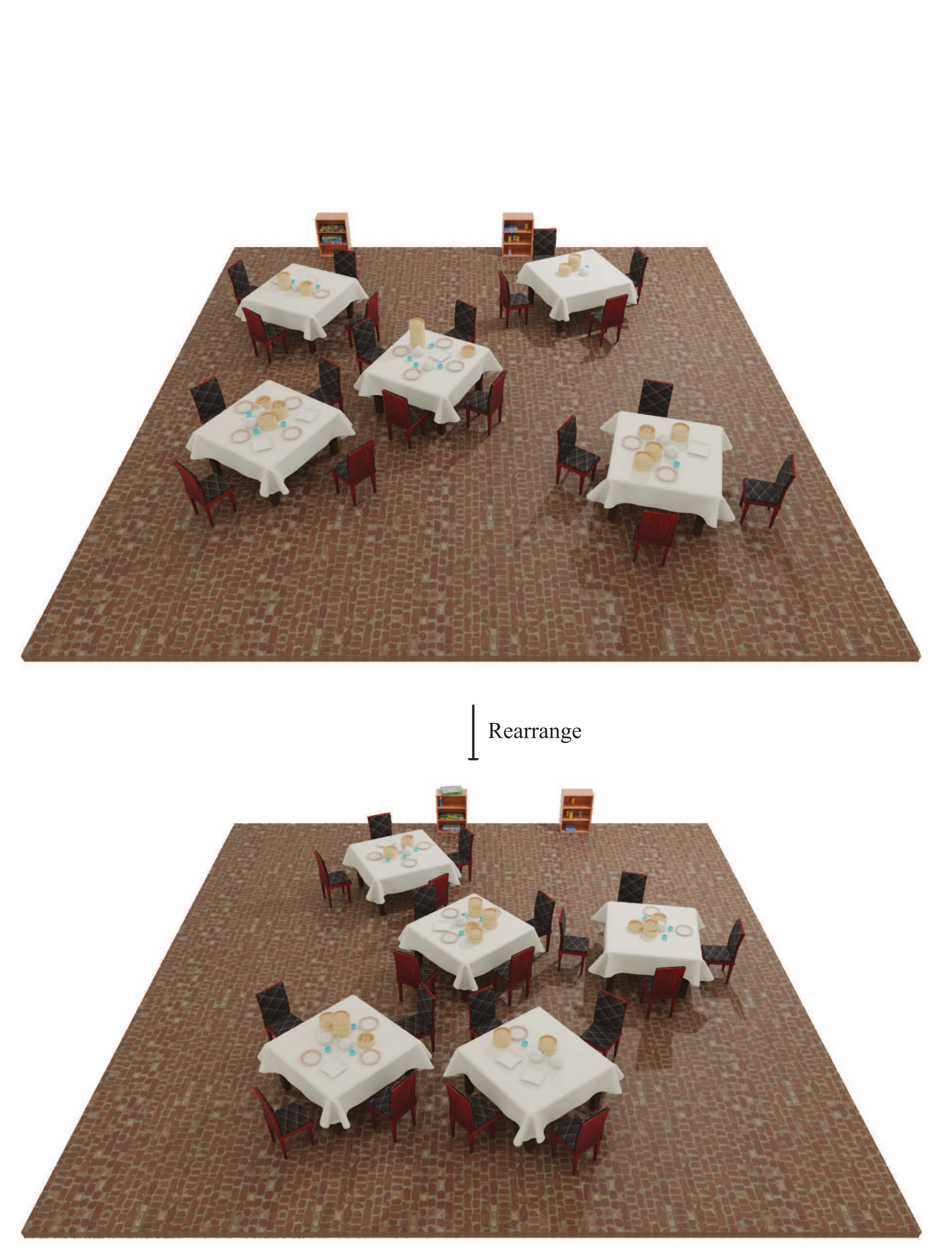
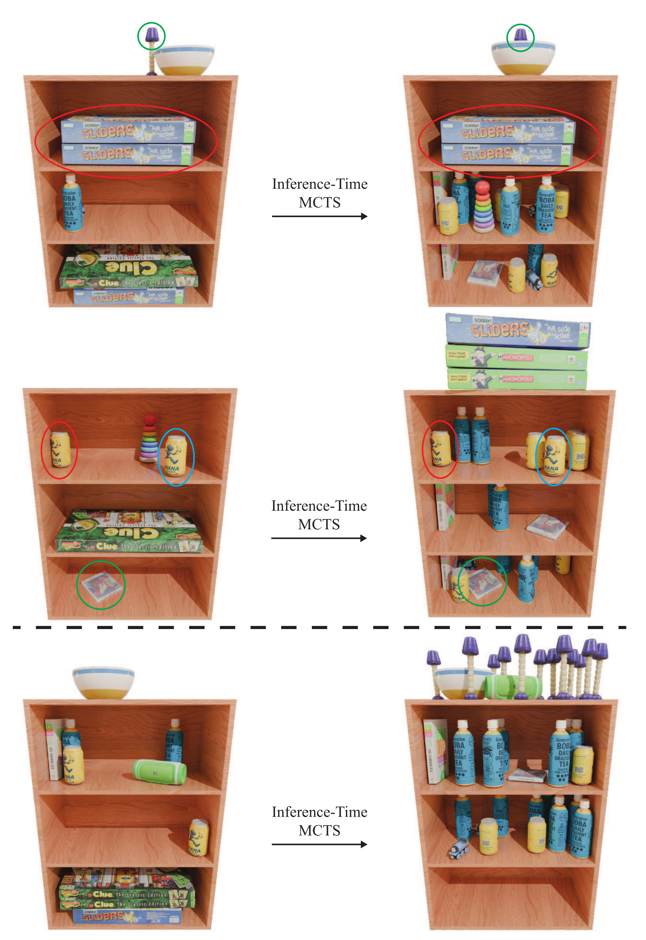
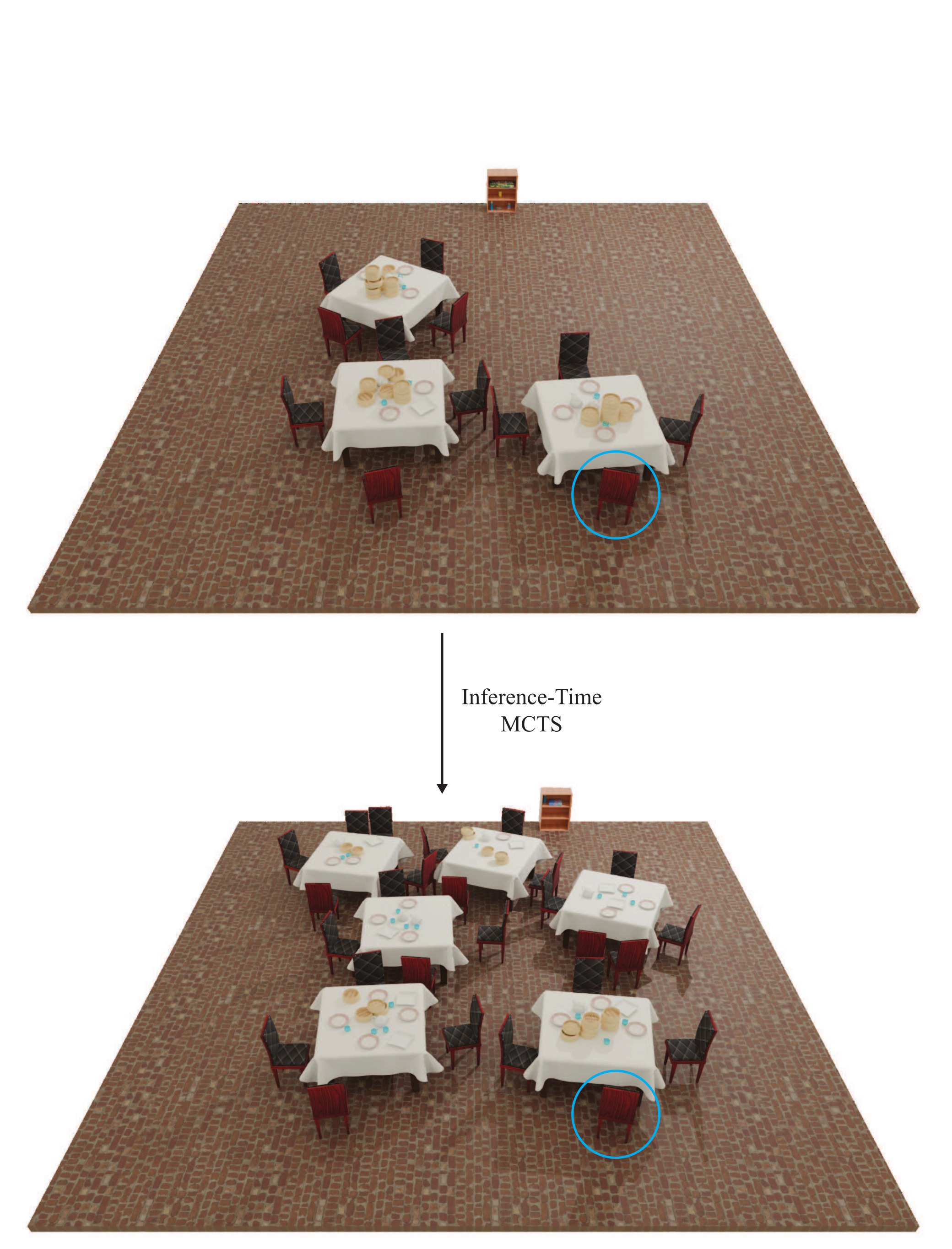
Additional search examples increase clutter while retaining portions of an initial scene. One shelf setting adds 30 object slots before search. A high-clutter restaurant example retains only a highlighted chair, showing that satisfying the objective can require replacing almost the entire initial scene.
The retained captions and panels document these individual searches. They do not report average runtime, success rates or quality at matched compute against alternative optimizers.
D.5 Can We Generate Novel Scenes?
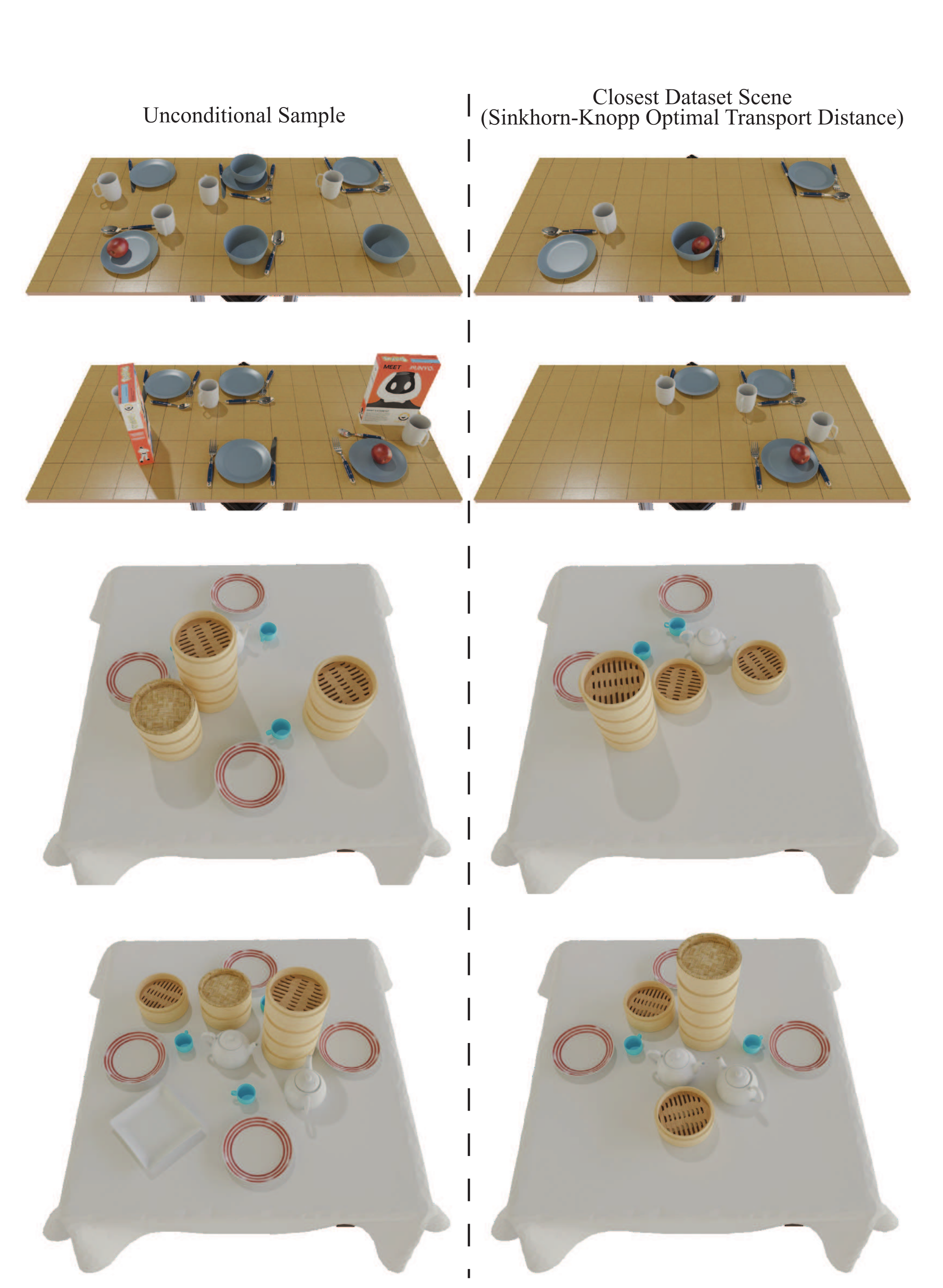
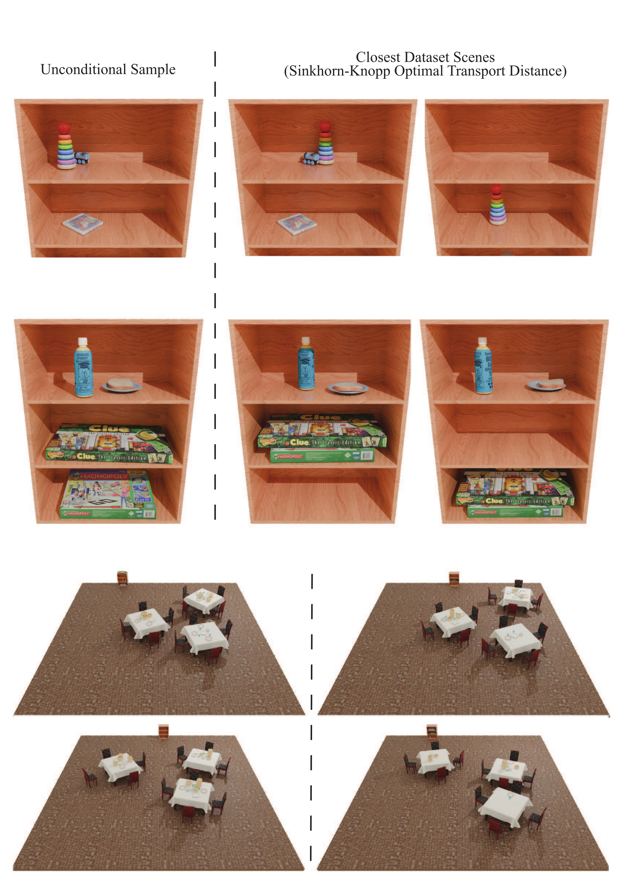
Generated object sets are compared with nearest training scenes using a Sinkhorn approximation to optimal transport, which respects permutation invariance. The displayed pairs differ in assets or poses, supporting novelty for these examples.
Selected nearest-neighbor comparisons are evidence against exact memorization in the shown samples, rather than a comprehensive test of overfitting or real-world generalization. The asset library remains fixed.
Appendix E Ablations
Ablations vary diffusion objective, rotation representation, numerical precision and physical repair. These separate distribution-matching improvements from geometric repair behavior.
E.1 Training Objective
The mixed objective improves CA and FID over the continuous-only variant in Tables 10–11. Continuous diffusion has slightly lower pre-repair penetration for low-clutter breakfast and dimsum scenes, illustrating that visual metrics and geometry need not improve together.
Table 11 labels living-room CA with 25 classifier iterations, whereas the corresponding main table uses 100 for the same mixed-model value. The original labels and values are retained; this inconsistency limits interpretation of that stated setting.
E.2 Rotation Representation
Nine-dimensional rotations followed by SVD projection improve CA and FID over axis-angle and quaternion alternatives on both tested datasets. They do not minimize every metric: axis-angle has lower pre-repair breakfast penetration, while quaternion has lower category KL there.
| Method | Breakfast Table (Low-Clutter Variant) | Living Room Shelf | ||||||
|---|---|---|---|---|---|---|---|---|
| CA (25 it, %) | KL () | FID | MTP (cm) | CA (100 it, %) | KL () | FID | MTP (cm) | |
| Axis-Angle | 66.57 ± 6.97 | 1.25 | 2.51 | 3.25 | 69.91 ± 3.90 | 2.61 | 2.20 | 0.03 |
| Quaternion | 61.38 ± 7.64 | 1.00 | 2.46 | 3.31 | 61.58 ± 4.61 | 2.53 | 2.10 | 0.03 |
| +SVD | 57.85 ± 4.98 | 1.67 | 2.39 | 3.50 | 52.84 ± 1.26 | 2.13 | 2.09 | 0.02 |
E.3 Training Precision
Full precision improves CA, FID and penetration over the tested bfloat16 configuration, especially on room-scale layouts. Evaluation uses each model’s training precision, so this comparison changes training and sampling precision together. The original “ft32” table label is retained.
The living-room full-precision FID is listed as 2.10 here versus 2.09 elsewhere. This small source discrepancy is preserved rather than silently reconciled.
E.4 Post Processing Pipeline
Figure 34 compares the same initial scenes with no repair, simulation alone, and projection followed by simulation. Simulation can disperse or destabilize deeply penetrating configurations; projection first better preserves the intended layout in the selected examples.
The authors deliberately choose scenes with prominent initial violations. This qualitative ablation explains the repair order but does not quantify its average success rate or eliminate the convergence failures discussed in Appendix B.