Literature
Display
← All papers

Dexterous Contact-Rich Manipulation via the Contact Trust Region

H. J. Terry Suh · Tao Pang · Tong Zhao · Russ Tedrake

Preprint posted · arXiv (preprint) ↗

Robotics17 min text · CondensedOriginal paper ↗
Contents

At a glance

Contact Trust Region augments a local linear contact-dynamics model with constraints on predicted contact forces and motion. Unlike a symmetric ellipsoidal bound alone, it can reject directions that require unilateral contact to pull. A relaxed version supports local trajectory optimization and feedback control; a roadmap connects useful local plans for broader reorientation. Experiments cover planar bimanual manipulation and a three-dimensional dexterous hand. The reported efficiency depends on supplied geometry, models, and task structure, rather than learning a general manipulation policy.

1 Introduction

The central question is where a differentiable contact simulator’s local approximation remains physically meaningful. Sensitivity analysis already enforces linearized force balance and perturbed complementarity, but a Taylor model alone can omit primal and dual feasibility. Contact Trust Region restores those convex constraints, connecting differentiable simulation with classical contact-force reasoning. The paper builds a local conic trajectory optimizer and a roadmap from these models, then evaluates planning, stabilization, and longer traversals separately. Its low computational cost is a result for the modeled tasks and chosen comparisons, not a universal dominance claim over reinforcement learning.
Refer to caption
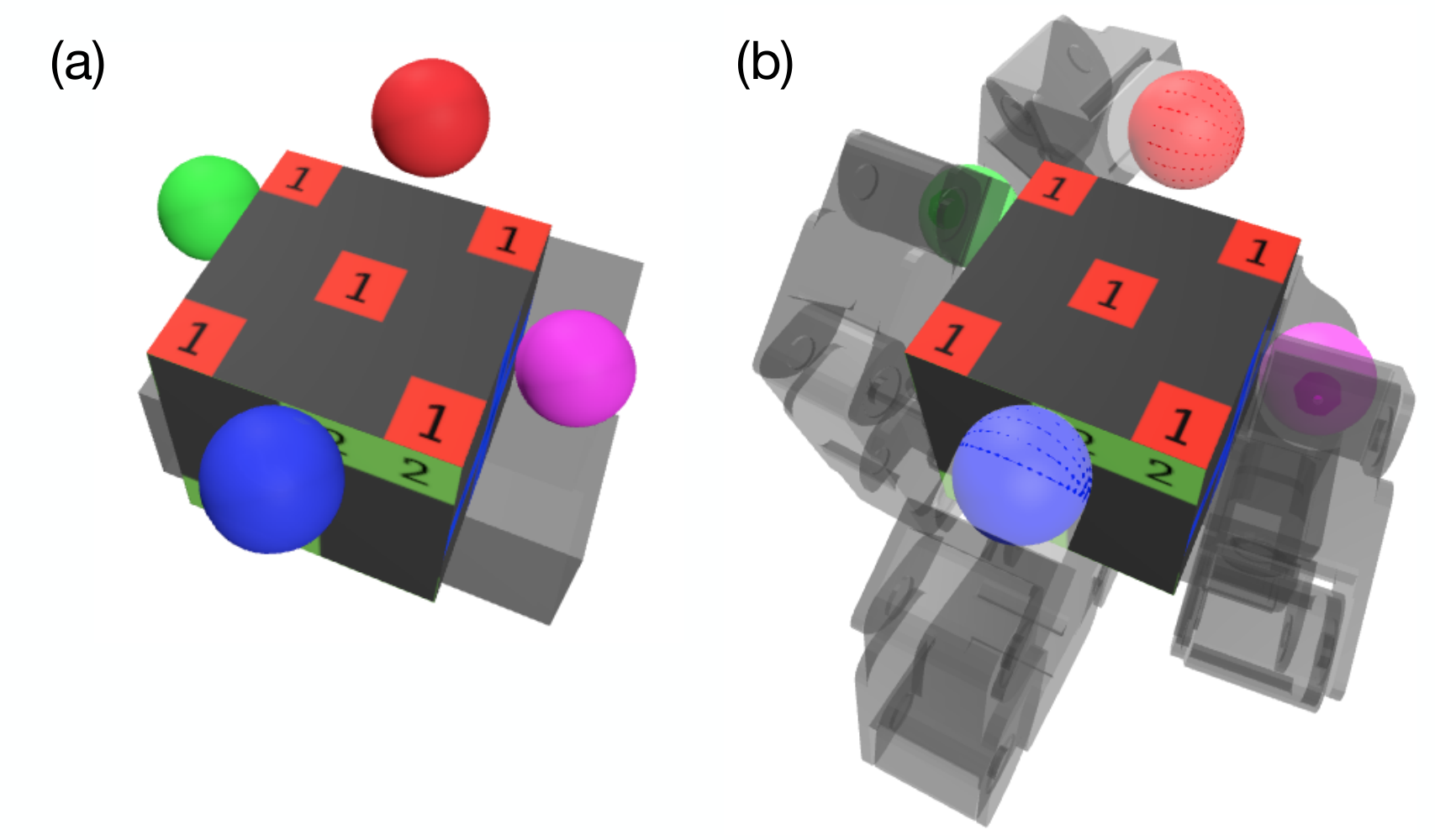
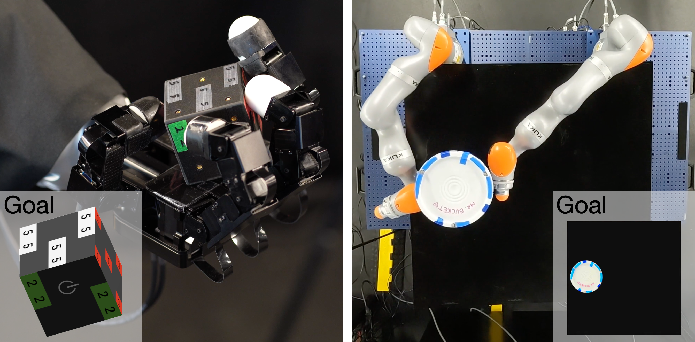
Figure 1: Hardware experiments illustrating the utility of our proposed method in contact-rich manipulation. Left: Dexterous in-hand manipulation with the Allegro hand moving a cube. Right: Whole-body manipulation with bimanual iiwas moving a bucket.
Table 1: List of Symbols
Symbol Shape Meaning
nqn_{q} ℕ\mathbb{N} number of positions in a system
nqan_{q^{\mathrm{a}}} ℕ\mathbb{N} number of actuated positions
nqon_{q^{\mathrm{o}}} ℕ\mathbb{N} number of object positions
qq ℝnq\mathbb{R}^{n_{q}} system configuration vector, q≔(qa,qo)q\coloneqq({q^{\mathrm{a}}},{q^{\mathrm{o}}})
qa{q^{\mathrm{a}}} ℝnqa\mathbb{R}^{n_{q_{\mathrm{a}}}} actuated (robot) configuration vector
qo{q^{\mathrm{o}}} ℝnqo\mathbb{R}^{n_{q_{\mathrm{o}}}} object configuration vector
q+o/aq_{+}^{\mathrm{o}/\mathrm{a}} ℝnqo/nqa\mathbb{R}^{n_{q_{\mathrm{o}}}/n_{q_{\mathrm{a}}}} object/robot configuration at the next step
uu ℝnqa\mathbb{R}^{n_{q_{\mathrm{a}}}} control input
λi\lambda_{i} ℝ3\mathbb{R}^{3} contact force at contact ii, λi≔(λni,λti)\lambda_{i}\coloneqq(\lambda_{\mathrm{n}_{i}},\lambda_{\mathrm{t}_{i}})
λni\lambda_{\mathrm{n}_{i}} ℝ\mathbb{R} normal contact force at contact ii
λti\lambda_{\mathrm{t}_{i}} ℝ2\mathbb{R}^{2} tangential contact force at contact ii
ϕi\phi_{i} ℝ\mathbb{R} signed distance at contact ii, (5a)
τo/a\tau^{\mathrm{o}/\mathrm{a}} ℝnqo/nqa\mathbb{R}^{n_{q_{\mathrm{o}}}/n_{q_{\mathrm{a}}}} non-contact torque acting on object/robot
hh ℝ+\mathbb{R}_{+} step size in seconds
𝐊a\mathbf{K}_{\mathrm{a}} 𝐒+⁣+nqa\mathbf{S}^{n_{q_{\mathrm{a}}}}_{++} robot stiffness matrix
𝐌o\mathbf{M}_{\mathrm{o}} 𝐒+⁣+nqo\mathbf{S}^{n_{q_{\mathrm{o}}}}_{++} object mass matrix
𝐉i\mathbf{J}_{i} ℝ3×nq\mathbb{R}^{3\times n_{q}} contact Jacobian at contact ii, (2)
𝒦i\mathcal{K}_{i} ℝ3\mathbb{R}^{3} feasible velocity cone at contact ii, (4a)
𝒦i⋆\mathcal{K}_{i}^{\star} ℝ3\mathbb{R}^{3} friction cone at contact ii, (4b)
μi\mu_{i} ℝ+\mathbb{R}_{+} friction coefficient at contact ii
νi\nu_{i} ℝ3\mathbb{R}^{3} (5a)
𝐏\mathbf{P} 𝐒+⁣+nq\mathbf{S}^{n_{q}}_{++} quadratic cost in contact dynamics, (3b)
bb nqn_{q} linear cost in contact dynamics, (3c)
cic_{i} ℝ3\mathbb{R}^{3} (7c)
κ\kappa ℝ+\mathbb{R}_{+} contact dynamics smoothing parameter
f(κ)​(⋅,⋅)f_{(\kappa)}(\cdot,\cdot) ℝnq×ℝnqa\mathbb{R}^{n_{q}}\times\mathbb{R}^{n_{q_{\mathrm{a}}}} (κ\kappa-smoothed) contact dynamics, ((14))(8)
→ℝnq\rightarrow\mathbb{R}^{n_{q}}
𝐀(κ)\mathbf{A}_{(\kappa)} ℝnq×nq\mathbb{R}^{n_{q}\times n_{q}} ∂f(κ)/∂q\partial f_{(\kappa)}/\partial q
𝐁(κ)\mathbf{B}_{(\kappa)} ℝnq×nqa\mathbb{R}^{n_{q}\times n_{q_{\mathrm{a}}}} ∂f(κ)/∂u\partial f_{(\kappa)}/\partial u
𝐂(κ),i\mathbf{C}_{(\kappa),i} ℝnq×nq\mathbb{R}^{n_{q}\times n_{q}} ∂λ(κ),i/∂q\partial\lambda_{(\kappa),i}/\partial q
𝐃(κ),i\mathbf{D}_{(\kappa),i} ℝnq×nqa\mathbb{R}^{n_{q}\times n_{q_{\mathrm{a}}}} ∂λ(κ),i/∂u\partial\lambda_{(\kappa),i}/\partial u
⋅¯\bar{\cdot} N.A. nominal quantities, e.g. q¯\bar{q}, see (17)
δ⋅\delta{\cdot} N.A. deviation from nominal quantities, e.g. δ​q\delta{q}
⋅^\hat{\cdot} N.A. Taylor expansions, e.g. q^+\hat{q}_{+}
𝚺\mathbf{\Sigma} 𝐒+⁣+(nq+nqa)\mathbf{S}_{++}^{(n_{q}+n_{q_{\mathrm{a}}})} trust region radius
ℰ𝚺\mathcal{E}_{\mathbf{\Sigma}} ℝnq+nqa\mathbb{R}^{n_{q}+n_{q_{\mathrm{a}}}} ETR with radius 𝚺\mathbf{\Sigma}, (22)
𝒮𝚺,κ\mathcal{S}_{\mathbf{\Sigma},\kappa} ℝnq+nqa\mathbb{R}^{n_{q}+n_{q_{\mathrm{a}}}} CTR with radius 𝚺\mathbf{\Sigma} and smoothing κ\kappa, (24)
𝒮𝚺,κ𝒜\mathcal{S}_{\mathbf{\Sigma},\kappa}^{\mathcal{A}} ℝnqa\mathbb{R}^{n_{q_{\mathrm{a}}}} Action-only CTR, (25)
𝒮~𝚺,κ\tilde{\mathcal{S}}_{\mathbf{\Sigma},\kappa} ℝnq+nqa\mathbb{R}^{n_{q}+n_{q_{\mathrm{a}}}} Relaxed CTR, (26)
𝒮~𝚺,κ𝒜\tilde{\mathcal{S}}_{\mathbf{\Sigma},\kappa}^{\mathcal{A}} ℝnqa\mathbb{R}^{n_{q_{\mathrm{a}}}} Relaxed Action-only CTR, (27)
ℳ𝚺,κ(𝒜)\mathcal{M}_{\mathbf{\Sigma,\kappa}}^{(\mathcal{A})} ℝnq\mathbb{R}^{n_{q}} (action-only) motion set, ((29))(28)
𝒞𝚺,κ,i𝒜\mathcal{C}^{\mathcal{A}}_{\mathbf{\Sigma},\kappa,i} ℝ3\mathbb{R}^{3} contact force set at contact ii, (30)
𝒥​𝒞𝚺,κ,i𝒜\mathcal{JC}^{\mathcal{A}}_{\mathbf{\Sigma},\kappa,i} ℝnqo\mathbb{R}^{n_{q_{\mathrm{o}}}} generalized friction cone at contact ii, (31)
𝒲𝚺,κ𝒜\mathcal{W}^{\mathcal{A}}_{\mathbf{\Sigma},\kappa} ℝnqo\mathbb{R}^{n_{q_{\mathrm{o}}}} wrench set, (32)
ℳ𝚺,κ𝒜,o\mathcal{M}^{\mathcal{A},\mathrm{o}}_{\mathbf{\Sigma},\kappa} ℝnqo\mathbb{R}^{n_{q_{\mathrm{o}}}} motion set projected to the space of qo{q^{\mathrm{o}}}, (33)
TT ℕ\mathbb{N} CtrTrajOpt planning horizon in Algorithm 1
nmaxn_{\mathrm{max}} ℕ\mathbb{N} CtrTrajOpt iteration limit in Algorithm 1
HH ℕ\mathbb{N} MPC rollout horizon in Algorithm 2
rr ℝ+\mathbb{R}_{+} scalar trust region radius in Section 5.2.1
𝐐\mathbf{Q} 𝐒+nq\mathbf{S}_{+}^{n_{q}} state tracking quadratic in (37)
𝐑\mathbf{R} 𝐒+nqa\mathbf{S}_{+}^{n_{q_{\mathrm{a}}}} control action quadratic cost in (37)
NN ℕ\mathbb{N} number of MPC re-plans in Algorithm 3

2 Preliminaries: Contact Dynamics as Convex Optimization

The derivation uses convex quasidynamic contact simulation: configurations evolve under a strongly damped approximation without explicit velocity state. This makes each step an optimization problem whose primal solution gives motion and whose dual quantities represent contact forces. The subsequent trust region inherits both the efficiency and the approximations of this model. See Pang et al. (2023) for the cited foundation.

2.1 Setup & Notation

Configuration coordinates split into actuated robot joints and unactuated object coordinates. An action is a desired joint configuration sent to a stiffness controller, with diagonal gains. Velocities are omitted under the quasidynamic assumption; the resulting state and input are therefore different from those of a general second-order rigid-body simulator.

2.2 Equations of Motion

Force balance relates commanded stiffness forces, external loads, contact impulses, and object displacement. Contact Jacobians map generalized coordinates into normal and tangential contact directions, while a regularization term makes the object’s quasi-static displacement response well-defined. The model uses contact pairs found by collision detection and treats each force as an average over the simulation step.

Equations 1a–3c
𝐊a​(q+a−u)\displaystyle\mathbf{K}_{\mathrm{a}}({q^{\mathrm{a}}_{\texttt{+}}}-u) =τa+∑i=1nc(𝐉ai​(q))⊤​λi\displaystyle=\tau^{\mathrm{a}}+\sum^{n_{c}}_{i=1}(\mathbf{J}_{\mathrm{a}_{i}}(q))^{\top}\lambda_{i} (1a)
ϵ​𝐌o​(q)​q+o−qoh2\displaystyle\epsilon\mathbf{M}_{\mathrm{o}}(q)\frac{{q^{\mathrm{o}}_{\texttt{+}}}-{q^{\mathrm{o}}}}{h^{2}} =τo+∑i=1nc(𝐉oi​(q))⊤​λi\displaystyle=\tau^{\mathrm{o}}+\sum^{n_{c}}_{i=1}(\mathbf{J}_{\mathrm{o}_{i}}(q))^{\top}\lambda_{i} (1b)
𝐉i≔[𝐉oi,𝐉ai]≔[𝐉ni𝐉ti]∈ℝ3×nq.\mathbf{J}_{i}\coloneqq[\mathbf{J}_{\mathrm{o}_{i}},\mathbf{J}_{\mathrm{a}_{i}}]\coloneqq\begin{bmatrix}\mathbf{J}_{\mathrm{n}_{i}}\\ \mathbf{J}_{\mathrm{t}_{i}}\end{bmatrix}\in\mathbb{R}^{3\times n_{q}}. (2)
𝐏⁡(q)​q++b⁡(q,u)−∑i=1nc𝐉i​(q)⊤​λi=0,where\displaystyle\mathbf{P}(q){q_{\texttt{+}}}+b(q,u)-\sum_{i=1}^{n_{c}}\mathbf{J}_{i}(q)^{\top}\lambda_{i}=0,\;\text{where} (3a)
𝐏⁡(q)≔[ϵ​𝐌o​(q)/h200𝐊a],\displaystyle\mathbf{P}(q)\coloneqq\begin{bmatrix}\epsilon\mathbf{M}_{\mathrm{o}}(q)/h^{2}&0\\ 0&\mathbf{K}_{\mathrm{a}}\end{bmatrix}, (3b)
b⁡(q,u)≔−[ϵ​𝐌o​(q)​qo/h2+τo𝐊a​u+τa].\displaystyle b(q,u)\coloneqq-\begin{bmatrix}\epsilon\mathbf{M}_{\mathrm{o}}(q){q^{\mathrm{o}}}/h^{2}+\tau^{\mathrm{o}}\\ \mathbf{K}_{\mathrm{a}}u+\tau^{\mathrm{a}}\end{bmatrix}. (3c)

2.3 Contact Constraints

Contact must satisfy non-penetration, friction-cone feasibility, and complementarity between separation and force, with friction opposing motion. The convex relaxation expresses these through dual cones. It introduces a modeling artifact: tangential sliding can induce normal separation. Thus the convenient convex formulation is an approximation to physical contact, not an exact general friction law. See Anitescu (2006) for the cited foundation.

Equations 4a–5c
𝒦i\displaystyle\mathcal{K}_{i} ≔{νi=(νni,νti)∈ℝ3|νni≥μi​νti⊤​νti},\displaystyle\coloneqq\left\{\nu_{i}=(\nu_{\mathrm{n}_{i}},\nu_{\mathrm{t}_{i}})\in\mathbb{R}^{3}|\nu_{\mathrm{n}_{i}}\geq\mu_{i}\sqrt{\nu_{\mathrm{t}_{i}}^{\top}\nu_{\mathrm{t}_{i}}}\right\}, (4a)
𝒦i⋆\displaystyle\mathcal{K}_{i}^{\star} ≔{λi=(λni,λti)∈ℝ3|μi​λni≥λti⊤​λti}.\displaystyle\coloneqq\left\{\lambda_{i}=(\lambda_{\mathrm{n}_{i}},\lambda_{\mathrm{t}_{i}})\in\mathbb{R}^{3}|\mu_{i}\lambda_{\mathrm{n}_{i}}\geq\sqrt{\lambda_{\mathrm{t}_{i}}^{\top}\lambda_{\mathrm{t}_{i}}}\right\}. (4b)
νi≔𝐉i​(q)​(q+−q)+[ϕi,0,0]⊤\displaystyle\nu_{i}\coloneqq\mathbf{J}_{i}(q)({q_{\texttt{+}}}-q)+[\phi_{i},0,0]^{\top} ∈𝒦i,\displaystyle\in\mathcal{K}_{i}, (5a)
λi\displaystyle\lambda_{i} ∈𝒦i⋆,\displaystyle\in\mathcal{K}_{i}^{\star}, (5b)
νi⊤​λi\displaystyle\nu_{i}^{\top}\lambda_{i} =0,\displaystyle=0, (5c)

2.4 Contact Dynamics as Convex Optimization

The contact equations are the optimality conditions of a second-order cone program. Its primal solution supplies the next configuration, while dual feasibility restricts contact forces. Complementary slackness here is orthogonality of the cone vectors, rather than requiring every corresponding component to vanish separately. This optimization view makes the dynamics a parameterized solution map.

Equations 6a–8b
find\displaystyle\mathrm{find}\quad q+\displaystyle q_{+} (6a)
s.t. (3),(5a),(5b),(5c).\displaystyle\eqref{eq:balance_single_equation},\eqref{eq:friction_constraints:primal_feasibility},\eqref{eq:friction_constraints:dual_feasibility},\eqref{eq:friction_constraints:complementary_slackness}. (6b)
min.q+​12​q+⊤​𝐏​(q)​q++b​(q,u)⊤​q+,subject to\displaystyle\underset{{q_{\texttt{+}}}}{\mathrm{min}.}\;\frac{1}{2}{q_{\texttt{+}}}^{\top}\mathbf{P}(q){q_{\texttt{+}}}+b(q,u)^{\top}{q_{\texttt{+}}},\;\text{subject to} (7a)
𝐉i(q)q++ci(q)∈𝒦i,∀i∈ℐc,where\displaystyle\qquad\mathbf{J}_{i}(q){q_{\texttt{+}}}+c_{i}(q)\in\mathcal{K}_{i},\;\forall i\in\mathcal{I}_{c},\;\text{where} (7b)
ci​(q)≔[ϕi​(q),0,0]⊤−𝐉i​(q)​q.\displaystyle c_{i}(q)\coloneqq[\phi_{i}(q),0,0]^{\top}-\mathbf{J}_{i}(q)q. (7c)
q+=\displaystyle q_{+}= f⁡(q,u)\displaystyle f(q,u) (8a)
=\displaystyle= argminq+​12​q+⊤​𝐏​(q)​q++b​(q,u)⊤​q+,\displaystyle\text{argmin}_{q_{+}}\;\;\frac{1}{2}q_{+}^{\top}\mathbf{P}(q)q_{+}+b(q,u)^{\top}q_{+},
subject to​𝐉i​(q)​q++ci​(q)∈𝒦i,∀i∈ℐc.\displaystyle\text{subject to}\;\;\mathbf{J}_{i}(q)q_{+}+c_{i}(q)\in\mathcal{K}_{i},\forall i\in\mathcal{I}_{c}. (8b)
Due to the quasidynamic assumption, velocity is omitted from the state, which only consists of the system configuration qq. We sometimes omit the explicit dependence of 𝐏,b,𝐉i\mathbf{P},b,\mathbf{J}_{i}, and cic_{i} on (q,u)(q,u) when it is clear from context.

2.5 Smoothing of Contact Dynamics

Contact-mode changes produce discontinuous gradients and flat regions that hinder local optimization. Log-barrier relaxation smooths the dynamics by perturbing complementarity, yielding forces even before bodies touch. These artificial forces provide directions for optimization, while their dual interpretation still respects the friction cone. Smoothing improves numerical tractability but introduces physical bias that must be controlled.

Equations 9–14b
λκ,i⊤​νi=2​κ−1.\lambda_{\kappa,i}^{\top}\nu_{i}=2\kappa^{-1}. (9)
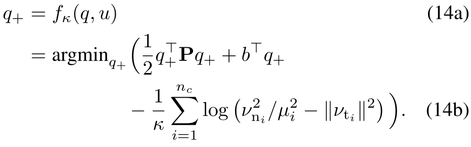
minq+⁡12​q+⊤​𝐏​q++b⊤​q+−1κ​∑i=1nclog⁡(νni2/μi2−‖νti‖2),\min_{q_{+}}\;\frac{1}{2}q_{+}^{\top}\mathbf{P}q_{+}+b^{\top}q_{+}-\frac{1}{\kappa}\sum^{n_{c}}_{i=1}\log\left(\nu_{\mathrm{n}_{i}}^{2}/\mu_{i}^{2}-\|\nu_{\mathrm{t}_{i}}\|^{2}\right), (10)
𝐏​q++b−∑i=1nc2​κ−1νni2/μi2−‖νti‖2​𝐉i⊤​[νni/μi2−νti]=0.\mathbf{P}q_{+}+b-\sum_{i=1}^{n_{\mathrm{c}}}\frac{2\kappa^{-1}}{\nu_{\mathrm{n}_{i}}^{2}/\mu_{i}^{2}-\|\nu_{\mathrm{t}_{i}}\|^{2}}\mathbf{J}_{i}^{\top}\begin{bmatrix}\nu_{\mathrm{n}_{i}}/\mu_{i}^{2}\\ -\nu_{\mathrm{t}_{i}}\\ \end{bmatrix}=0. (11)
λκ,i=2​κ−1νni2/μi2−‖νti‖2​[νni/μi2−νti].\lambda_{\kappa,i}=\frac{2\kappa^{-1}}{\nu_{\mathrm{n}_{i}}^{2}/\mu_{i}^{2}-\|\nu_{\mathrm{t}_{i}}\|^{2}}\begin{bmatrix}\nu_{\mathrm{n}_{i}}/\mu_{i}^{2}\\ -\nu_{\mathrm{t}_{i}}\end{bmatrix}. (12)
𝐏​q++b−∑i=1nc𝐉i⊤​λκ,i=0,\mathbf{P}q_{+}+b-\sum_{i=1}^{n_{c}}\mathbf{J}_{i}^{\top}\lambda_{\kappa,i}=0, (13)
Original PDF equation 14 with complete source notation and layout.

2.6 Sensitivity Analysis of Smoothed Contact Dynamics

Sensitivity analysis differentiates the stationarity and perturbed-complementarity equations, then applies the implicit-function theorem to obtain derivatives of both next configuration and contact force. Action derivatives are simpler; state derivatives also involve the changing contact Jacobian and geometric curvature. The force derivatives become essential information for the proposed trust region.

Equation 15
[𝐏ℋi​[−𝐉i⊤]𝒱i​[λi⊤​𝐉i]𝒟i​[(𝐉i​q++ci)⊤]]​[∂q+∂u𝒱i​[∂λκ,i∂u]]=[−∂b∂u0]\displaystyle\begin{bmatrix}\mathbf{P}&\mathcal{H}_{i}\left[-\mathbf{J}_{i}^{\top}\right]\\ \mathcal{V}_{i}\left[\lambda^{\top}_{i}\mathbf{J}_{i}\right]&\mathcal{D}_{i}\left[\left(\mathbf{J}_{i}q_{+}+c_{i}\right)^{\top}\right]\end{bmatrix}\begin{bmatrix}\frac{\partial{q_{+}}}{\partial{u}}\\ \mathcal{V}_{i}\left[\frac{\partial{\lambda_{\kappa,i}}}{\partial{u}}\right]\end{bmatrix}=\begin{bmatrix}-\frac{\partial{b}}{\partial{u}}\\ 0\end{bmatrix} (15)

3 Local Approximation of Contact Dynamics

A local optimizer needs a tractable substitute for a dynamics constraint that is itself defined by an optimization problem. The paper studies the validity of joint local models of motion and force, then separates small-perturbation accuracy from contact feasibility.

Equations 16a–16b
minq+,u\displaystyle\min_{q_{+},u}\quad ‖qgoal−q+‖2\displaystyle\|q_{\mathrm{goal}}-q_{+}\|^{2} (16a)
s.t. q+=f⁡(q,u).\displaystyle q_{+}=f(q,u). (16b)

3.1 Linear Model over Smoothed Primal and Dual Variables

Taylor expansions of both primal motion and dual contact force satisfy the linearized force-balance and perturbed-complementarity equalities to first order. The lemma follows by combining nominal optimality with the sensitivity equations and discarding higher-order terms. It does not establish exact nonlinear dynamics or feasibility for arbitrary perturbations; those remaining inequalities motivate the trust region.

Equations 17a–21
q^+\displaystyle\hat{q}_{+} =𝐀​δ​q+𝐁​δ​u+f⁡(q¯,u¯),\displaystyle=\mathbf{A}\delta q+\mathbf{B}\delta u+f(\bar{q},\bar{u}), (17a)
𝐀\displaystyle\mathbf{A} ≔∂f/∂q⁡(q¯,u¯),𝐁≔∂f/∂u⁡(q¯,u¯),\displaystyle\coloneqq\partial f/\partial q(\bar{q},\bar{u}),\;\;\mathbf{B}\coloneqq\partial f/\partial u(\bar{q},\bar{u}), (17b)
δ​q\displaystyle\delta q ≔q−q¯,δ​u≔u−u¯.\displaystyle\coloneqq q-\bar{q},\;\;\delta u\coloneqq u-\bar{u}. (17c)
q^+\displaystyle\hat{q}_{+} =𝐀κ​δ​q+𝐁κ​δ​u+fκ​(q¯,u¯),\displaystyle=\mathbf{A}_{\kappa}\delta q+\mathbf{B}_{\kappa}\delta u+f_{\kappa}(\bar{q},\bar{u}), (18a)
𝐀κ\displaystyle\mathbf{A}_{\kappa} ≔∂fκ/∂q⁡(q¯,u¯),𝐁κ≔∂fκ/∂u⁡(q¯,u¯),\displaystyle\coloneqq\partial f_{\kappa}/\partial q(\bar{q},\bar{u}),\;\;\mathbf{B}_{\kappa}\coloneqq\partial f_{\kappa}/\partial u(\bar{q},\bar{u}), (18b)
λ^+,i\displaystyle\hat{\lambda}_{+,i} =𝐂κ,i​δ​q+𝐃κ,i​δ​u+λκ,i​(q¯,u¯),\displaystyle=\mathbf{C}_{\kappa,i}\delta q+\mathbf{D}_{\kappa,i}\delta u+\lambda_{\kappa,i}(\bar{q},\bar{u}), (19a)
𝐂κ,i\displaystyle\mathbf{C}_{\kappa,i} ≔∂λκ,i/∂q⁡(q¯,u¯),𝐃κ,i≔∂λκ,i/∂u⁡(q¯,u¯).\displaystyle\coloneqq\partial\lambda_{\kappa,i}/\partial q(\bar{q},\bar{u}),\;\;\mathbf{D}_{\kappa,i}\coloneqq\partial\lambda_{\kappa,i}/\partial u(\bar{q},\bar{u}). (19b)
[q^+𝒱i​[λ^+,i]]=[𝐀κ𝐁κ𝒱i​[𝐂κ,i]𝒱i​[𝐃κ,i]]​[δ​qδ​u]+[fκ​(q¯,u¯)𝒱i​[λκ,i​(q¯,u¯)]].\displaystyle\begin{bmatrix}\hat{q}_{+}\\ \mathcal{V}_{i}[\hat{\lambda}_{+,i}]\end{bmatrix}=\begin{bmatrix}\mathbf{A}_{\kappa}&\mathbf{B}_{\kappa}\\ \mathcal{V}_{i}[\mathbf{C}_{\kappa,i}]&\mathcal{V}_{i}[\mathbf{D}_{\kappa,i}]\end{bmatrix}\begin{bmatrix}\delta q\\ \delta u\end{bmatrix}+\begin{bmatrix}f_{\kappa}(\bar{q},\bar{u})\\ \mathcal{V}_{i}[\lambda_{\kappa,i}(\bar{q},\bar{u})]\end{bmatrix}. (20)
[𝐏^​q^++b^−∑i=1nc𝐉^i⊤​λ^+,i𝒱i​[(𝐉^i​q^++c^i)⊤​λ^+,i−2​κ−1]]=𝒪⁡((δ​q,δ​u)2)\displaystyle\begin{bmatrix}\hat{\mathbf{P}}\hat{q}_{+}+\hat{b}-\sum^{n_{c}}_{i=1}\hat{\mathbf{J}}_{i}^{\top}\hat{\lambda}_{+,i}\\ \mathcal{V}_{i}\left[(\hat{\mathbf{J}}_{i}\hat{q}_{+}+\hat{c}_{i})^{\top}\hat{\lambda}_{+,i}-2\kappa^{-1}\right]\end{bmatrix}=\mathcal{O}\left((\delta q,\delta u)^{2}\right) (21)

3.2 Ellipsoidal Trust Region (ETR)

An ellipsoidal bound limits how far state and input perturbations move from the nominal point. Its image through a linear model is another ellipsoid, so it is symmetric even when contact permits motion only in one direction. Large ellipsoids risk approximation error, while shrinking them to fit the feasible set can make progress unnecessarily slow.

Equations 22–23
ℰ𝚺​(q¯,u¯)≔{δ​z=(δ​q,δ​u)|δ​z⊤​𝚺​δ​z≤1}.\mathcal{E}_{\mathbf{\Sigma}}(\bar{q},\bar{u})\coloneqq\{\delta z=(\delta q,\delta u)|\delta z^{\top}\mathbf{\Sigma}\delta z\leq 1\}. (22)
{q^+|q^+=𝐀κδq+𝐁κδu+fκ(q¯,u¯),(δq,δu)∈ℰ𝚺(q¯,u¯)}\displaystyle\{\hat{q}_{+}|\hat{q}_{+}=\mathbf{A}_{\kappa}\delta q+\mathbf{B}_{\kappa}\delta u+f_{\kappa}(\bar{q},\bar{u}),(\delta q,\delta u)\in\mathcal{E}_{\mathbf{\Sigma}}(\bar{q},\bar{u})\} (23)

3.3 Contact Trust Region (CTR)

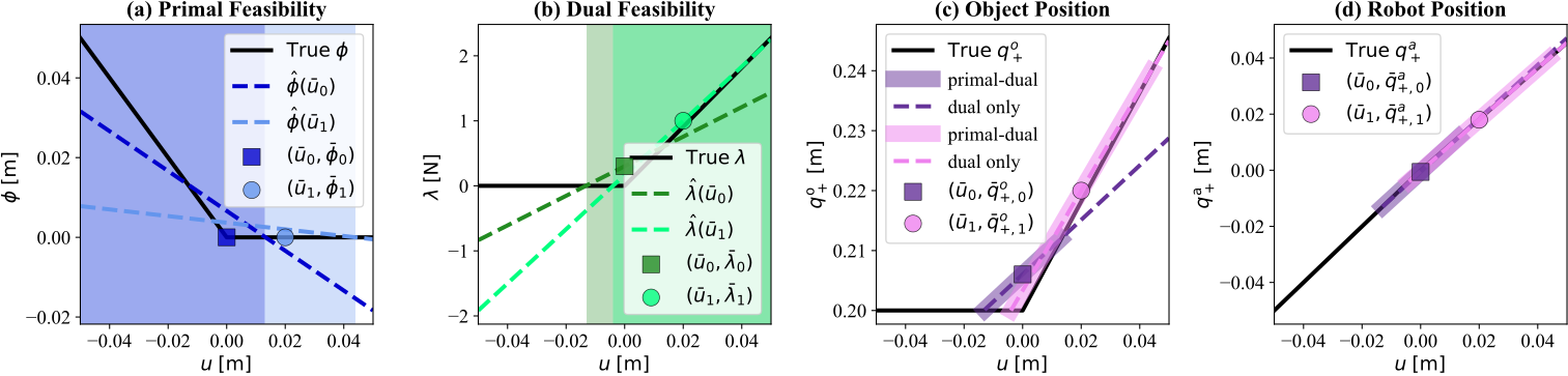
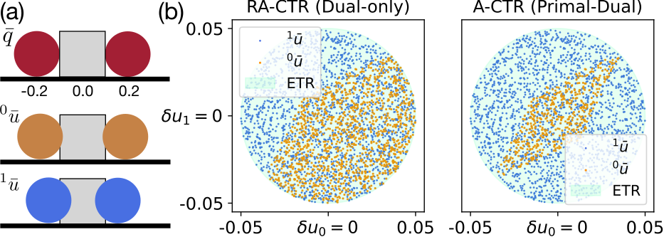
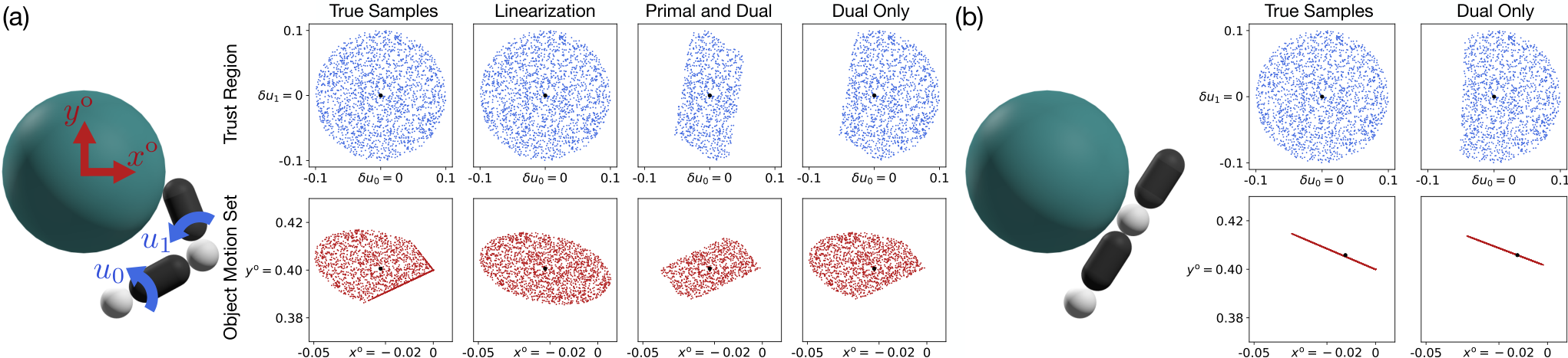
The full Contact Trust Region intersects an ellipsoidal perturbation bound with linearized motion and force feasibility. For a fixed current configuration, its action-only version removes state perturbations. Convexity follows from the affine models and cone constraints; equivalence to the smoothed contact equations is local and first order. Pushing examples show why dual feasibility blocks most fictitious pulling, while smoothing can leave a small mismatch. They also show that linearized non-penetration may be overly conservative. In squeezing, stronger nominal contact can instead leave the entire ellipsoid feasible, so the added constraints do not always shrink it.

Equations 24a–25e
𝒮𝚺,κ(q¯,u¯)≔{\displaystyle\mathcal{S}_{\mathbf{\Sigma},\kappa}(\bar{q},\bar{u})\coloneqq\{ (δq,δu)|δz⊤𝚺δz≤1,δz=(δq,δu),\displaystyle(\delta q,\delta u)|\delta z^{\top}\mathbf{\Sigma}\delta z\leq 1,\delta z=(\delta q,\delta u), (24a)
q^+\displaystyle\hat{q}_{+} =𝐀κ​δ​q+𝐁κ​δ​u+fκ​(q¯,u¯),\displaystyle=\mathbf{A}_{\kappa}\delta q+\mathbf{B}_{\kappa}\delta u+f_{\kappa}(\bar{q},\bar{u}), (24b)
λ^+,i\displaystyle\hat{\lambda}_{+,i} =𝐂κ,i​δ​q+𝐃κ,i​δ​u+λκ,i​(q¯,u¯),\displaystyle=\mathbf{C}_{\kappa,i}\delta q+\mathbf{D}_{\kappa,i}\delta u+\lambda_{\kappa,i}(\bar{q},\bar{u}), (24c)
𝐉^i​q^++c^i\displaystyle\hat{\mathbf{J}}_{i}\hat{q}_{+}+\hat{c}_{i} ∈𝒦i,\displaystyle\in\mathcal{K}_{i}, (24d)
λ^+,i\displaystyle\hat{\lambda}_{+,i} ∈𝒦i⋆}.\displaystyle\in\mathcal{K}^{\star}_{i}\}. (24e)
𝒮𝚺,κ𝒜(q¯,u¯)≔{δu|\displaystyle\mathcal{S}^{\mathcal{A}}_{\mathbf{\Sigma},\kappa}(\bar{q},\bar{u})\coloneqq\{\delta u| δ​u⊤​𝚺​δ​u≤1,\displaystyle\delta u^{\top}\mathbf{\Sigma}\delta u\leq 1, (25a)
q^+\displaystyle\hat{q}_{+} =𝐁κ​δ​u+fκ​(q¯,u¯),\displaystyle=\mathbf{B}_{\kappa}\delta u+f_{\kappa}(\bar{q},\bar{u}), (25b)
λ^+,i\displaystyle\hat{\lambda}_{+,i} =𝐃κ,i​δ​u+λκ,i​(q¯,u¯),\displaystyle=\mathbf{D}_{\kappa,i}\delta u+\lambda_{\kappa,i}(\bar{q},\bar{u}), (25c)
𝐉i​q^++ci\displaystyle\mathbf{J}_{i}\hat{q}_{+}+c_{i} ∈𝒦i,\displaystyle\in\mathcal{K}_{i}, (25d)
λ^+,i\displaystyle\hat{\lambda}_{+,i} ∈𝒦i⋆}.\displaystyle\in\mathcal{K}^{\star}_{i}\}. (25e)
Original figure
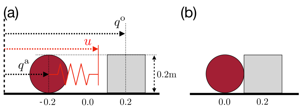
Figure 2: A-CTR illustrations for the system in Figure 3b at (q¯o,q¯a)=(0.2,0)(\bar{q}^{\mathrm{o}},\bar{q}^{\mathrm{a}})=(0.2,0). Sub-figures show how (a) the signed distance function ϕ\phi, (b) the contact force λ\lambda, (c) the object configuration q+o{q^{\mathrm{o}}_{\texttt{+}}} and (d) the robot configuration q+a{q^{\mathrm{a}}_{\texttt{+}}} change as a function of the action uu. In every sub-figure, the black solid line represents the true, non-smooth dynamics (8). The markers (squares and circles) represent linearization points. In (a) and (b), the deeper-colored dotted lines represent the linearization at u¯0=0\bar{u}_{0}=0, and the lighter-colored lines represent the linearization at u¯1=0.02\bar{u}_{1}=0.02. The shaded regions represent the feasible set of the corresponding color. For instance, the dark blue shaded region in (a) represents ϕ^​(q¯=(0.2,0),u¯=0)≥0\hat{\phi}\left(\bar{q}=(0.2,0),\bar{u}=0\right)\geq 0; the light green region in (b) represents λ^+​(q¯=(0.2,0),u¯=0.02)≥0\hat{\lambda}_{+}\left(\bar{q}=(0.2,0),\bar{u}=0.02\right)\geq 0. In (c) and (d), the dotted lines show parts of the linearizations that satisfy only the dual constraints; the thick shaded lines around dotted lines satisfy both the primal and dual constraints.
Original PDF figure 3 with complete source notation and layout.
Figure 3: (a) Schematic of the 1-dimensional pusher system used in Example 1. (b) corresponds to the configuration (qo,qa)=(0.2,0)({q^{\mathrm{o}}},{q^{\mathrm{a}}})=(0.2,0).
Original figure
Figure 4: (a) Nominal configuration and actions for Example 2. u0u_{0} and u1u_{1} are the position commands of the left and right ball, respectively. (b) Samples in the action space that satisfy the primal (24d) and dual (24e) feasibility constraints for different nominal actions.

3.4 Relaxed Contact Trust Region (R-CTR)

The relaxed variants retain friction-cone constraints on predicted contact forces but omit primal non-penetration feasibility. This often avoids an overly small region caused by unequal smoothed sensitivities of robot and object. The motion set is the convex image of that relaxed region through the local dynamics. Examples match one-step object motion and manipulator singularities better than either a symmetric ellipsoid or the full region, but dropping primal feasibility means the relaxed set is not a general certificate of exact collision-free motion.

Equations 26a–28b
𝒮~𝚺,κ(q¯,u¯)≔{\displaystyle\tilde{\mathcal{S}}_{\mathbf{\Sigma},\kappa}(\bar{q},\bar{u})\coloneqq\{ (δq,δu)|δz⊤𝚺δz≤1,δz=(δq,δu),\displaystyle(\delta q,\delta u)|\delta z^{\top}\mathbf{\Sigma}\delta z\leq 1,\delta z=(\delta q,\delta u), (26a)
q^+\displaystyle\hat{q}_{+} =𝐀κ​δ​q+𝐁κ​δ​u+fκ​(q¯,u¯),\displaystyle=\mathbf{A}_{\kappa}\delta q+\mathbf{B}_{\kappa}\delta u+f_{\kappa}(\bar{q},\bar{u}), (26b)
λ^+,i\displaystyle\hat{\lambda}_{+,i} =𝐂κ,i​δ​q+𝐃κ,i​δ​u+λκ,i​(q¯,u¯),\displaystyle=\mathbf{C}_{\kappa,i}\delta q+\mathbf{D}_{\kappa,i}\delta u+\lambda_{\kappa,i}(\bar{q},\bar{u}), (26c)
λ^+,i\displaystyle\hat{\lambda}_{+,i} ∈𝒦i⋆}.\displaystyle\in\mathcal{K}^{\star}_{i}\}. (26d)
𝒮~𝚺,κ𝒜(q¯,u¯)≔{δu|\displaystyle\tilde{\mathcal{S}}^{\mathcal{A}}_{\mathbf{\Sigma},\kappa}(\bar{q},\bar{u})\coloneqq\{\delta u| δ​u⊤​𝚺​δ​u≤1,\displaystyle\delta u^{\top}\mathbf{\Sigma}\delta u\leq 1, (27a)
q^+\displaystyle\hat{q}_{+} =𝐁κ​δ​u+fκ​(q¯,u¯),\displaystyle=\mathbf{B}_{\kappa}\delta u+f_{\kappa}(\bar{q},\bar{u}), (27b)
λ^+,i\displaystyle\hat{\lambda}_{+,i} =𝐃κ,i​δ​u+λκ,i​(q¯,u¯),\displaystyle=\mathbf{D}_{\kappa,i}\delta u+\lambda_{\kappa,i}(\bar{q},\bar{u}), (27c)
λ^+,i\displaystyle\hat{\lambda}_{+,i} ∈𝒦i⋆}.\displaystyle\in\mathcal{K}^{\star}_{i}\}. (27d)
ℳ𝚺,κ(q¯,u¯)≔{q^+|\displaystyle\mathcal{M}_{\mathbf{\Sigma,\kappa}}(\bar{q},\bar{u})\coloneqq\{\hat{q}_{+}| q^+=𝐀κ​δ​q+𝐁κ​δ​u+fκ​(q¯,u¯),\displaystyle\hat{q}_{+}=\mathbf{A}_{\kappa}\delta q+\mathbf{B}_{\kappa}\delta u+f_{\kappa}(\bar{q},\bar{u}), (28a)
(δq,δu)∈𝒮~𝚺,κ(q¯,u¯)}.\displaystyle(\delta q,\delta u)\in\tilde{\mathcal{S}}_{\mathbf{\Sigma},\kappa}(\bar{q},\bar{u})\}. (28b)
Refer to caption
Figure 5: Visualization of the A-CTR 𝒮𝚺,κ𝒜\mathcal{S}^{\mathcal{A}}_{\mathbf{\Sigma},\kappa} (primal and dual), RA-CTR 𝒮~𝚺,κ𝒜\tilde{\mathcal{S}}^{\mathcal{A}}_{\mathbf{\Sigma},\kappa} (dual only) and the action-only object motion set ℳΣ,κ𝒜,o\mathcal{M}^{\mathcal{A},\mathrm{o}}_{\mathrm{\Sigma},\kappa} under the different linearization points shown in the illustrations. In the “Trust Region” row, the “True Samples” subplot is obtained by uniformly sampling 2000 points from the ball ‖δ​u‖≤0.1\left\lVert{\delta u}\right\rVert\leq 0.1; samples in the following columns are obtained by rejecting samples that do not satisfy the respective constraints. In the “Object Motion Set” row, the “True Samples” subplot is obtained by passing the δ​u\delta u samples from the trust region subplot above through the true contact dynamics (8); samples in the following columns are obtained by mapping the δ​u\delta u samples from the corresponding trust region subplot through the linear map defined in (29).
Equations 29a–29b
ℳ𝚺,κ𝒜(q¯,u¯)≔{q^+|\displaystyle\mathcal{M}^{\mathcal{A}}_{\mathbf{\Sigma,\kappa}}(\bar{q},\bar{u})\coloneqq\{\hat{q}_{+}| q^+=𝐁κ​δ​u+fκ​(q¯,u¯),\displaystyle\hat{q}_{+}=\mathbf{B}_{\kappa}\delta u+f_{\kappa}(\bar{q},\bar{u}), (29a)
δu∈𝒮~𝚺,κ𝒜(q¯,u¯)}.\displaystyle\delta u\in\tilde{\mathcal{S}}^{\mathcal{A}}_{\mathbf{\Sigma},\kappa}(\bar{q},\bar{u})\}. (29b)

3.5 Mechanics Derivation of the Motion Set

A complementary derivation starts with locally predicted feasible contact forces, maps them through contact Jacobians into object wrenches, and then maps net impulses into quasistatic displacement. This connects the motion set with classical wrench sets and motion cones. Bounds come from actuator perturbations and the local model rather than arbitrary independent force limits. The equivalence lemma concerns the stated quasidynamic, linearized construction, not a global reachable set of the full physical system.

Equations 30a–33b
𝒞𝚺,κ,i𝒜(q¯,u¯)≔{λ^+,i|\displaystyle\mathcal{C}^{\mathcal{A}}_{\mathbf{\Sigma},\kappa,i}(\bar{q},\bar{u})\coloneqq\big\{\hat{\lambda}_{+,i}| λ^+,i=𝐃κ,i​δ​u+λκ,i​(q¯,u¯)\displaystyle\hat{\lambda}_{+,i}=\mathbf{D}_{\kappa,i}\delta u+\lambda_{\kappa,i}(\bar{q},\bar{u}) (30a)
λ^+,i∈𝒦i⋆,\displaystyle\hat{\lambda}_{+,i}\in\mathcal{K}_{i}^{\star}, (30b)
δu⊤𝚺δu≤1}.\displaystyle\delta u^{\top}\mathbf{\Sigma}\delta u\leq 1\big\}. (30c)
𝒥𝒞𝚺,κ,i𝒜(q¯,u¯)≔{wi|wi=𝐉oi⊤λ+,i,λ+,i∈𝒞𝚺,κ,i𝒜}.\displaystyle\mathcal{JC}^{\mathcal{A}}_{\mathbf{\Sigma},\kappa,i}(\bar{q},\bar{u})\coloneqq\left\{w_{i}|w_{i}=\mathbf{J}_{\mathrm{o}_{i}}^{\top}\lambda_{+,i},\;\lambda_{+,i}\in\mathcal{C}^{\mathcal{A}}_{\mathbf{\Sigma},\kappa,i}\right\}. (31a)
𝒲𝚺,κ𝒜(q¯,u¯)≔{w|w\displaystyle\mathcal{W}^{\mathcal{A}}_{\mathbf{\Sigma},\kappa}(\bar{q},\bar{u})\coloneqq\{w|w =τo+∑iwi\displaystyle=\tau^{\mathrm{o}}+\textstyle\sum_{i}w_{i} (32a)
wi\displaystyle w_{i} ∈𝒥𝒞𝚺,κ,i𝒜(q¯,u¯)},\displaystyle\in\mathcal{JC}^{\mathcal{A}}_{\mathbf{\Sigma},\kappa,i}(\bar{q},\bar{u})\}, (32b)
ℳ𝚺,κ𝒜,o(q¯,u¯)={q^+o|\displaystyle\mathcal{M}^{\mathcal{A},\mathrm{o}}_{\mathbf{\Sigma},\kappa}(\bar{q},\bar{u})=\{\hat{q}_{+}^{\mathrm{o}}| ϵ​𝐌o​(q¯)​(q^+o−q¯o)/h=h​w,\displaystyle\epsilon\mathbf{M}_{\mathrm{o}}(\bar{q})\left(\hat{q}^{\mathrm{o}}_{+}-\bar{q}^{\mathrm{o}}\right)/h=hw, (33a)
w∈𝒲𝚺,κ𝒜(q¯,u¯)}.\displaystyle w\in\mathcal{W}^{\mathcal{A}}_{\mathbf{\Sigma},\kappa}(\bar{q},\bar{u})\}. (33b)

3.6 Additional Constraints

Joint-command and steady-state torque limits can further restrict the convex local problem. They constrain the same perturbations used for planning, helping keep its proposed commands within the robot model’s operating range.

3.6.1 Joint Limits

Joint limits are imposed on the commanded robot configurations through lower and upper bounds. This limits the position input, rather than independently proving every transient physical state remains inside its limits.

Equation 34
ql​ba≤u¯+δ​u≤qu​ba.q^{\mathrm{a}}_{lb}\leq\bar{u}+\delta u\leq q^{\mathrm{a}}_{ub}. (34)

3.6.2 Torque Limits

The paper imposes affine bounds on a steady-state torque estimate derived from command–position error. Its printed equation (35) uses the inverse of the stiffness matrix, although equation (1) defines stiffness multiplying that error; the original notation is retained and should be checked before implementation. The quasidynamic model also omits inertial transients, so these bounds are not a full dynamic actuator-load guarantee.

Equation 35
τl​b≤𝐊a−1​(q¯+a+𝐁a​δ​u−(u¯+δ​u))≤τu​b.\tau_{lb}\leq\mathbf{K}_{\mathrm{a}}^{-1}\left(\bar{q}^{\mathrm{a}}_{+}+\mathbf{B}^{\mathrm{a}}\delta u-(\bar{u}+\delta u)\right)\leq\tau_{ub}. (35)

4 Local Planning and Control

Local planning minimizes a trajectory objective under contact dynamics, input bounds, and an initial condition. The proposed iterative method replaces the non-smooth problem with smoothed linear dynamics and relaxed contact trust regions. This can traverse useful contact-mode changes without explicitly enumerating every mode sequence, while retaining local optimization’s dependence on initialization.

Equations 36a–36d
minq0:T,u0:T−1\displaystyle\min_{q_{0:T},u_{0:T-1}}\quad ‖qgoal−qT‖𝐐2+∑t=0T−1‖ut−ut−1‖𝐑2,\displaystyle\|q_{\text{goal}}-q_{T}\|^{2}_{\mathbf{Q}}+\sum^{T-1}_{t=0}\|u_{t}-u_{t-1}\|^{2}_{\mathbf{R}}, (36a)
s.t. qt+1=f⁡(qt,ut)∀t,\displaystyle q_{t+1}=f(q_{t},u_{t})\quad\forall t, (36b)
|ut−ut−1|≤η∀t,\displaystyle|u_{t}-u_{t-1}|\leq\eta\quad\forall t, (36c)
q0=q¯0,\displaystyle q_{0}=\bar{q}_{0}, (36d)

4.1 Trajectory Optimization with R-CTR

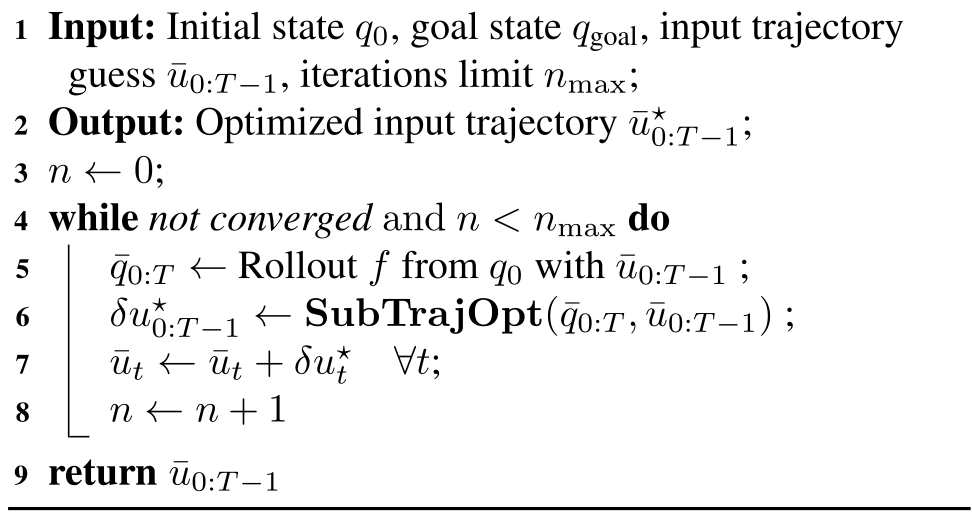
Each iteration rolls out a nominal input sequence, linearizes motion and force, and solves a conic optimization for all trajectory perturbations jointly. It then updates inputs and repeats the nonlinear rollout. The procedure resembles iterative linear-quadratic regulation but replaces its recursive backward pass with a joint constrained solve. The relaxed region is used because full primal feasibility often underestimates useful motion; additional joint or steady-state torque limits can be included. See Li and Todorov (2004) for the cited foundation.

Equations 37a–37h
SubTrajOpt(q¯0:T,u¯0:T−1,qgoal)=δu0:T−1⋆,where\displaystyle\mathrm{SubTrajOpt}(\bar{q}_{0:T},\bar{u}_{0:T-1},q_{\text{goal}})=\delta u^{\star}_{0:T-1},\text{where} (37a)
minδq0:T,δu0:T−1∥qgoal−qT∥2𝐐+∑T−1t=0∥ut−ut−1∥2𝐑,\displaystyle\min_{\delta q_{0:T},\delta u_{0:T-1}}\quad\|q_{\text{goal}}-q_{T}\|^{2}_{\mathbf{Q}}+\sum^{T-1}_{t=0}\|u_{t}-u_{t-1}\|^{2}_{\mathbf{R}}, (37b)
s.t.δ​qt+1=𝐀κ,t​δ​qt+𝐁κ,t​δ​ut,t=0​…​T−1,\displaystyle\text{s.t.}\quad\delta q_{t+1}=\mathbf{A}_{\kappa,t}\delta q_{t}+\mathbf{B}_{\kappa,t}\delta u_{t},\;t=0\dots T-1, (37c)
(δ​qt,δ​ut)∈𝒮~𝚺,κ​(q¯t,u¯t),t=0​…​T−1,\displaystyle\quad\quad(\delta q_{t},\delta u_{t})\in\tilde{\mathcal{S}}_{\mathbf{\Sigma,\kappa}}(\bar{q}_{t},\bar{u}_{t}),\;t=0\dots T-1, (37d)
qt=q¯t+δ​qt,t=0​…​T,\displaystyle\quad\quad q_{t}=\bar{q}_{t}+\delta q_{t},\;t=0\dots T, (37e)
ut=u¯t+δ​ut,t=0​…​T−1,\displaystyle\quad\quad u_{t}=\bar{u}_{t}+\delta u_{t},\;t=0\dots T-1, (37f)
|ut−ut−1|≤η,t=1​…​T−1,\displaystyle\quad\quad|u_{t}-u_{t-1}|\leq\eta,\;t=1\dots T-1, (37g)
δ​q0=0,\displaystyle\quad\quad\delta q_{0}=0, (37h)
Algorithm 1 CTR Trajectory Optimization-CtrTrajOpt
Original PDF algorithm 1 with complete source notation and layout.

4.2 Initial Guess Heuristic

When the robot starts far from the object, even smoothed motion gradients may be nearly zero. An initialization heuristic reverses the artificial barrier-force field and simulates the resulting attraction until contact is established, using relatively strong smoothing. This supplies a better starting command for the local optimizer; it is an initialization device, not a physically executed attractive contact force.

Equation 38
τ=−∑i𝐉oi⊤λi\tau=-\sum_{i}{\mathbf{J}^{\mathrm{o}}_{i}}^{\top}\lambda_{i} (38)

4.3 Examples

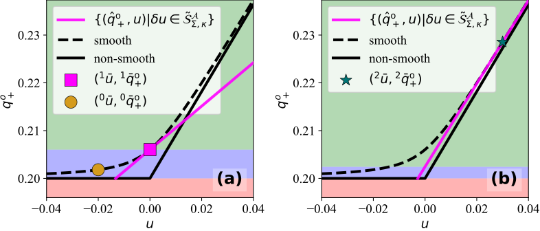
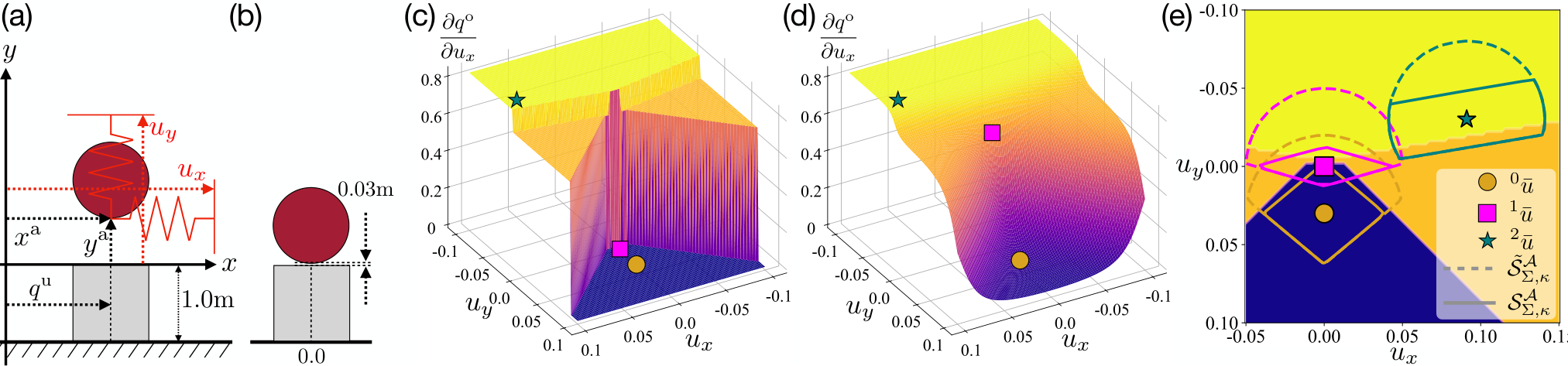
Toy pushing tasks illustrate how initialization and repeated relinearization can move an optimizer from separation into a useful sticking mode. Dual feasibility blocks impossible pulling, while stronger contact moves the nominal point away from the mode boundary and improves the local slope. Smoothing can still initially cause overshoot or even movement in the wrong direction for nearby goals. The examples explain a successful mechanism, not guaranteed convergence for arbitrary contact-rich tasks.
Original figure
Figure 6: Running Algorithm 1 on the 1D sphere-box system in Figure 3 from the nominal configuration (q¯0o,q¯0a)=(−0.02,0.2)(\bar{q}_{0}^{\mathrm{o}},\bar{q}_{0}^{\mathrm{a}})=(-0.02,0.2). In both subplots, the black solid line represents true non-smooth dynamics, and the black dashed line represents the smoothed dynamics. The yellow circle marks the naive nominal action u¯0=q¯0a{}^{0}\bar{u}=\bar{q}^{\mathrm{a}}_{0} and its resulting object configuration q¯0o0{}^{0}\bar{q}^{\mathrm{o}}_{0}. Similarly, the magenta square indicates the next nominal action u¯1{}^{1}\bar{u} after applying the initial guess heuristics, and the green star shows the final nominal action u¯2{}^{2}\bar{u} after running Algorithm 1. The magenta lines depict the set {(q^+,u¯+δu)|q^+=𝐁κδu+fκ(q¯,u¯),δu∈𝒮~𝚺,κ𝒜(q¯,u¯)}\{(\hat{q}_{+},\bar{u}+\delta u)|\hat{q}_{+}=\mathbf{B}_{\kappa}\delta u+f_{\kappa}(\bar{q},\bar{u}),\delta u\in\tilde{\mathcal{S}}^{\mathcal{A}}_{\mathbf{\Sigma},\kappa}(\bar{q},\bar{u})\} for the different nominal actions. The green, blue, red colored zones denote zones of qgoaloq^{\mathrm{o}}_{\text{goal}} where the inverse dynamics controller behaves similarly.
Refer to caption
Figure 7: (a) A schematic of the system in Example 5. (b) The nominal configuration q0o=0q^{\mathrm{o}}_{0}=0 and q0a=(x0a,y0a)=(0,0.03)q^{\mathrm{a}}_{0}=(x^{\mathrm{a}}_{0},y^{\mathrm{a}}_{0})=(0,0.03): the ball is hovering above but not touching the box. (c) Gradient landscape of the non-smooth dynamics at the nominal configuration in (b). The blue region at the bottom corresponds to the separation contact mode, the two orange regions the sliding modes, and the yellow region the sticking mode. (d) Gradient landscape of the smoothed dynamics at the same nominal configuration. The dynamics is smoothed with κ=1000\kappa=1000. (e) A-CTR (𝒮Σ,κ𝒜\mathcal{S}^{\mathcal{A}}_{\Sigma,\kappa}) and RA-CTR(𝒮~Σ,κ𝒜\tilde{\mathcal{S}}^{\mathcal{A}}_{\Sigma,\kappa}) for different u¯\bar{u}’s, overlaid on the non-smooth gradient landscape in (c).

4.4 Model Predictive Control

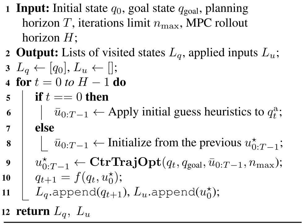
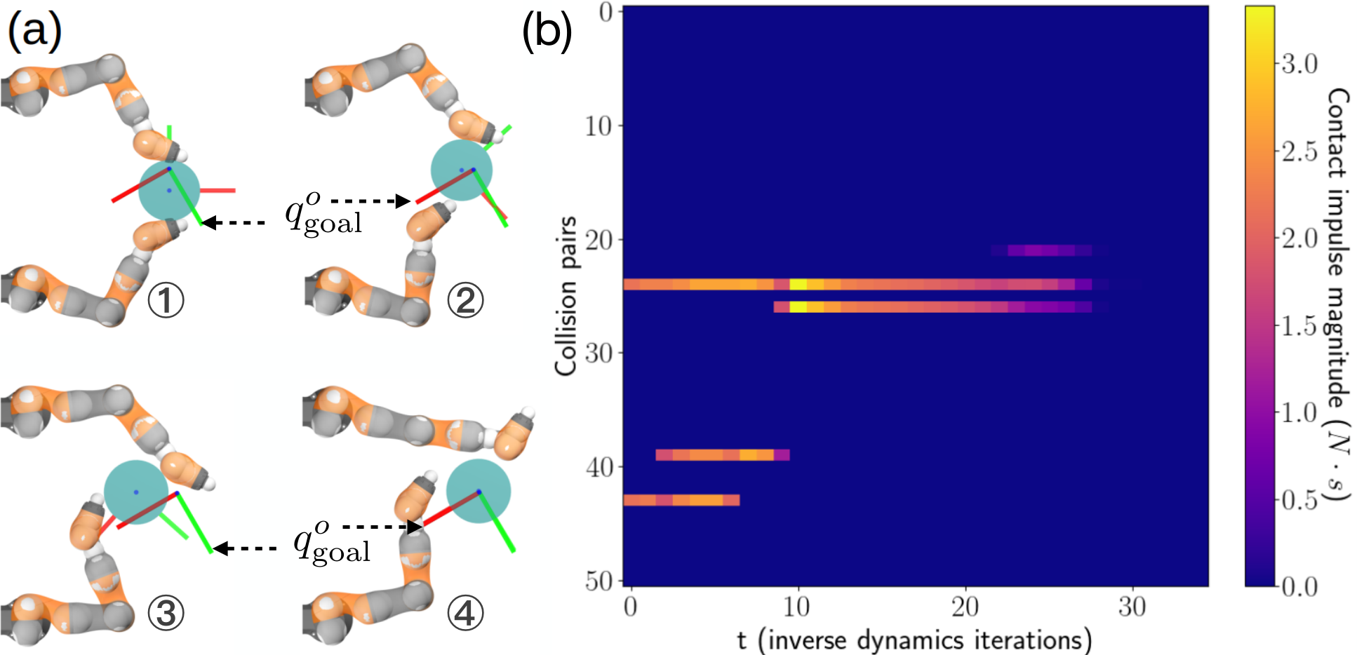
The trajectory optimizer becomes a receding-horizon controller by executing only its first command, observing the new configuration, and replanning. The first solve uses the contact initialization heuristic; later solves reuse the previous plan. A planar two-arm example changes contact modes while translating and rotating a cylinder. Planning horizon and total episode length are distinct, and stabilization under full second-order dynamics is evaluated separately later in the paper.
Algorithm 2 MPC Rollout (𝐌𝐏𝐂\mathbf{MPC})
Original PDF algorithm 2 with complete source notation and layout.
Refer to caption
Figure 8: Visualization for Example 6. (a) Visualization of key frames of the closed-loop sequence, with the current qoq^{\mathrm{o}} and the goal qgoaloq^{\mathrm{o}}_{\text{goal}} displayed as frames. (b) Visualization of contact forces of every potential collision pair in the IiwaBimanual system.

5 Local MPC Experiments

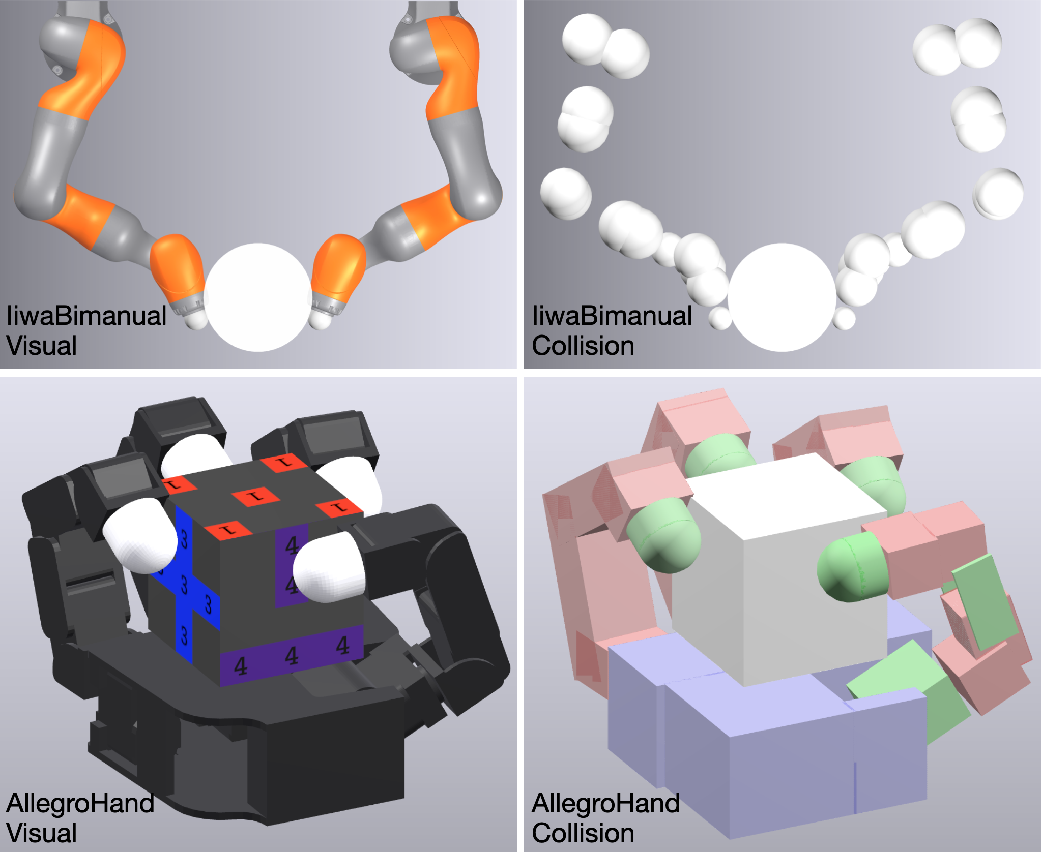
Local control is tested on planar bimanual manipulation with 6 actuated and 3 object degrees of freedom, and Allegro in-hand manipulation with 16 actuated and 6 object degrees of freedom. These experiments isolate the trust-region formulation under the same convex quasidynamic simulator used for planning; transfer to second-order dynamics is evaluated separately.
Refer to caption
Figure 9: Visual and collision geometries of IiwaBimanual (top) AllegroHand (bottom). Every IiwaBimanual geometry is shown as white, while the robot collision geometries in AllegroHand are colored to increase contrast.

5.1 Experiment Setup

Evaluation fixes diverse initial-state/goal pairs and compares final object-pose error across controllers. Robot joint targets are not prescribed, allowing each method to choose a useful grasping motion.

5.1.1 Goal Generation

Goals are deliberately locally reachable but challenging: roughly one thousand pairs per system cover broad pose differences. This is a test of local stabilization under a particular sampling scheme, rather than arbitrary global goals or an unbiased sample of all possible manipulation problems.

5.1.2 Evaluation Metrics

Final errors are reported separately as Euclidean translation distance and angular quaternion difference. Some plots add these numerically; that combined score mixes meters and radians and should be read alongside the separate quantities in the tables.

5.1.3 Implementation Details

Experiments use the authors’ existing open-source contact simulator and MOSEK for the conic subproblem, on an M2 Max laptop with 64 GB memory. Runtime claims refer to this model, implementation, and hardware. See MOSEK documentation for the cited foundation.

5.2 Effect of Trust Region Radius 𝚺 and Rollout Horizon H

The study varies trust-region radius and the number of executed MPC rollout steps while keeping the internal planning horizon at one. This separates local step authority from repeated feedback; increasing the internal horizon did not help the sampled bimanual goals in the appendix experiment.

5.2.1 Trust Region Radius

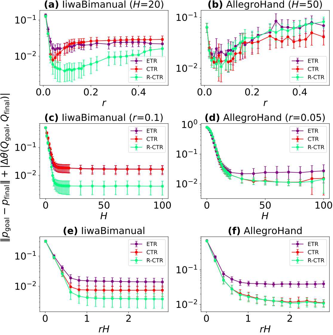
A tiny radius makes all three formulations similar but limits progress; an excessively large radius degrades the linear approximation. Relaxed contact feasibility gives the best bimanual results, while full and relaxed contact regions behave similarly for Allegro. The proposed explanation is that unilateral pushing exposes force constraints more strongly than stable opposing-finger grasps.
Original figure
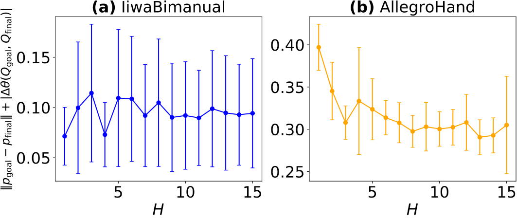
Figure 10: How tracking errors, defined as the sum of translation and rotation errors, change with different trust region radius rr (𝚺=r−2​𝐈\mathbf{\Sigma}=r^{-2}\mathbf{I}) and rollout horizon HH. The plotted curves denote the average error for the goals generated in Section 5.1.1, and the error bars denote 0.1​σ0.1\sigma where σ\sigma is the standard deviation. For plots (e) and (f), the plotted curves denote the best average error across all combinations of rr and HH with constant r⋅Hr\cdot H.

5.2.2 Rollout Horizon H

More rollout steps initially reduce error, followed by saturation. For Allegro, very long rollouts sometimes increase variance and error; the authors attribute this to numerical failures in its more numerous collision pairs. Longer execution is therefore not uniformly beneficial.

5.2.3 r ⋅ H : “Effective Lookahead”

The radius–rollout product is used as an approximate measure of how far repeated local actions can progress. Each plotted point selects the best radius/horizon combination at that product. Contact-constrained methods outperform the ellipsoidal baseline for sufficiently large products, but these best-of-sweep curves are not results for a single fixed controller tuning.
Refer to caption
(a) Iiwa Bimanual
Refer to caption
(b) Allegro Hand
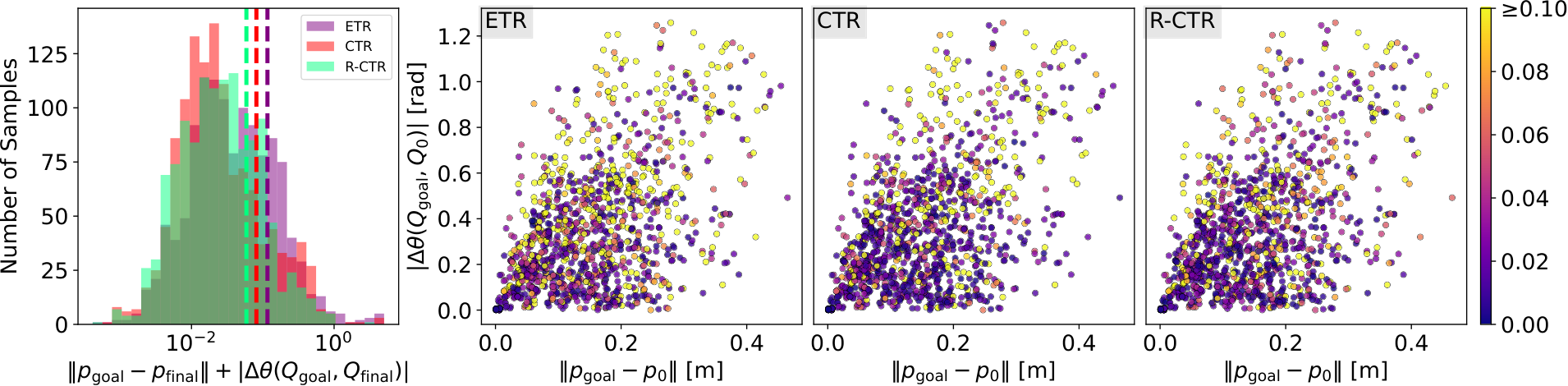
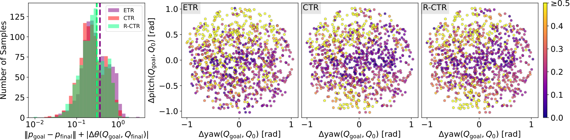
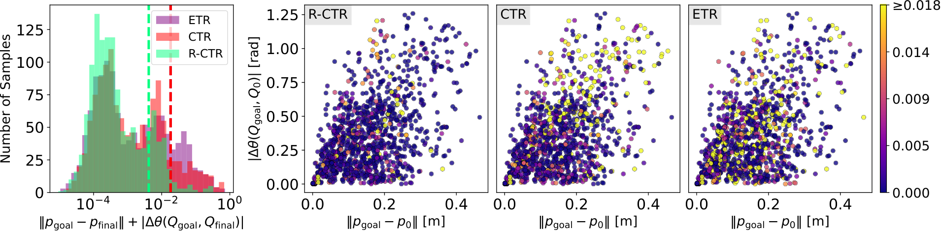
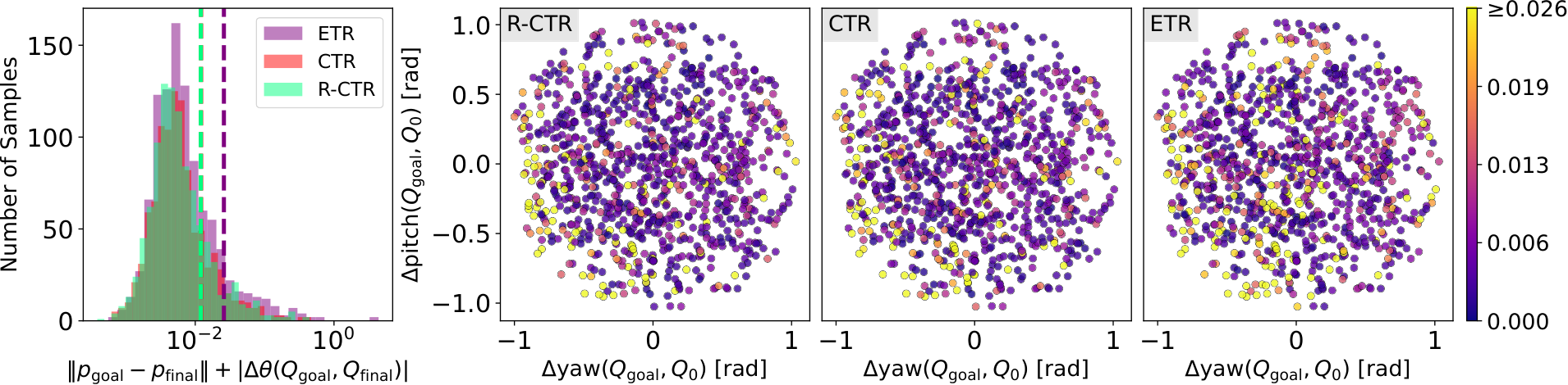
Figure 11: Results for running Algorithm 2 with R-CTR, CTR and ETR constraints on the pairs of goals and initial conditions generated in Section 5.1.1. The histogram shows how many samples reached a specified error in the xx axis, where error is defined as ‖pgoal−pfinal‖+|Δ​θ​(Qgoal,Qfinal)|\|p_{\text{goal}}-p_{\text{final}}\|+|\Delta\theta(Q_{\text{goal}},Q_{\text{final}})|. The dotted lines in the histogram represent the average errors. Some dotted lines are barely visible due to overlapping (their values are available in Table 3). Each dot in the scatter plot corresponds to a pair of an initial condition q0oq^{\mathrm{o}}_{0} and a goal qgoaloq^{\mathrm{o}}_{\text{goal}}. Color of the dots is determined by the error: warmer colors indicate bigger errors. The three scatter plots in each row share the same color scale, whose maximum value is the average of the errors for reaching the goals with ETR. (a) For IiwaBimanual, the xx axis of the scatter plots is the position difference between q0oq^{\mathrm{o}}_{0} and qgoaloq^{\mathrm{o}}_{\text{goal}}, the yy axis the angular difference. (b) For AllegroHand, as the position difference is small for all goals, the xx axis shows the yaw angle difference between q0oq^{\mathrm{o}}_{0} and qgoaloq^{\mathrm{o}}_{\text{goal}}, and the yy axis the pitch angle difference. The roll, pitch and yaw axes are defined in Figure 15a.

5.3 Can Our Method Reach Goals?

With selected hyperparameters, the relaxed region is compared with full contact feasibility and ellipsoidal bounds over every sampled pair. The figures show distributions as well as averages, making rare large errors visible.

System TT nmaxn_{\max} rr HH
IiwaBimanual 1 2 0.10 20
AllegroHand 1 3 0.05 50
Table 2: MPC hyperparameters: TT and nmaxn_{\mathrm{max}} are defined in Algorithm 1; rr is the trust region radius (𝚺=r−2​𝐈\mathbf{\Sigma}=r^{-2}\mathbf{I}); HH is the MPC rollout horizon in Algorithm 2.

5.3.1 Goal Tracking Performance

The relaxed region has the lowest mean and variance on both systems. Its advantage is especially clear for bimanual cases where the ellipsoidal baseline proposes motion that unilateral contact cannot produce. Allegro’s full and relaxed regions are nearly tied. The explanation for why primal feasibility is much more restrictive in one system remains a hypothesis about geometry and contact configuration.

IiwaBimanual AllegroHand
Trans. [mm] Rot. [mrad] Trans. [mm] Rot. [mrad]
R-CTR 2.0 (11.5) 2.1 (10.1) 2.2 (5.7) 9.8 (26.9)
CTR 9.4 (30.9) 8.9 (33.3) 2.2 (5.6) 9.9 (28.3)
ETR 8.6 (23.8) 9.6 (37.9) 4.5 (53.8) 21.4 (136.4)
Table 3: Mean translation and rotation errors for the combined errors in Figure 11. Each cell displays the mean (std).

5.3.2 Infeasibility

Infeasible local problems are rare in the reported runs, despite repeated construction of new regions. When one occurs, the rollout stops immediately. The empirical count is reassuring for these cases but does not establish recursive feasibility or guaranteed completion.

ETR CTR R-CTR Number of Goals
IiwaBimanual 0 0 0 1233
AllegroHand 5 2 3 1000
Table 4: Number of infeasible trust regions encountered while running Algorithm 2 to reach the goals from Section 5.1.1.

5.3.3 Computation Time

The unconstrained ellipsoidal variant is fastest, full contact feasibility slowest, and Allegro costs more than bimanual control. Constraint pruning and exploiting repeated sparsity are proposed optimizations. Reported timing includes the chosen conservative set of potential contacts.

Time unit [ms] IiwaBimanual AllegroHand
Per IGH 16.8 (0.05) 32.0 (0.6)
Per 𝐂𝐭𝐫𝐓𝐫𝐚𝐣𝐎𝐩𝐭\mathbf{CtrTrajOpt} R-CTR 5.1 (0.4) 99.2 (28.6)
CTR 7.0 (0.2) 205.7 (32.5)
ETR 2.4 (0.2) 52.9 (21.8)
Per qt+1=f⁡(qt,u0⋆)q_{t+1}=f(q_{t},u_{0}^{\star}) 0.9 (0.05) 5.92 (0.38)
Table 5: Breakdown of the average runtime (wall clock) for Algorithm 2. IGH stands for Initial Guess Heuristic. Each cell displays the mean (standard deviation).

6 Stabilization under Second-Order Dynamics

The next experiments test the model gap explicitly. Convex quasidynamic simulation omits inertia and permits sliding contact with a small separation gap, called hydroplaning. The controller is therefore evaluated in a second-order simulator without that artifact and on physical robots.

6.1 Implementation Heuristics for Second-order Dynamics

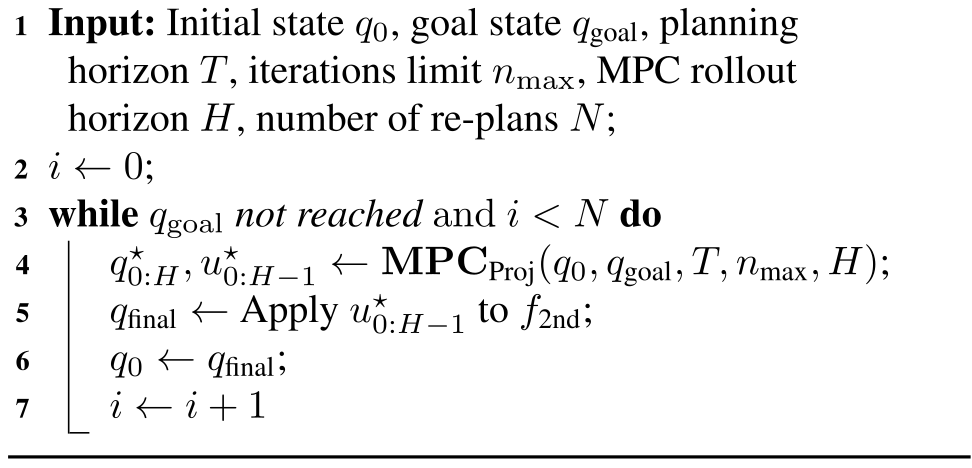
Two practical modifications improve transfer: execute short planned action chunks before replanning, and repeatedly use the contact-seeking initialization heuristic. The latter compensates for planned sliding forces that may not exist when the real fingers separate. These are empirical model-gap corrections, not a replacement with exact second-order contact dynamics.
Algorithm 3 MPC with 2nd-order Dynamics f2ndf_{\text{2nd}}
Original PDF algorithm 3 with complete source notation and layout.
Refer to caption
(a) IiwaBimanual: implementation heuristics ablation, all using R-CTR.
Refer to caption
(b) IiwaBimanual: closed-loop trust region comparison. R-CTR results are the same as the closed-loop results in (a).
Refer to caption
(c) AllegroHand: implementation heuristics ablation, all using R-CTR.
Refer to caption
(d) AllegroHand: closed-loop trust region comparison. R-CTR results are the same as the closed-loop results in (c).
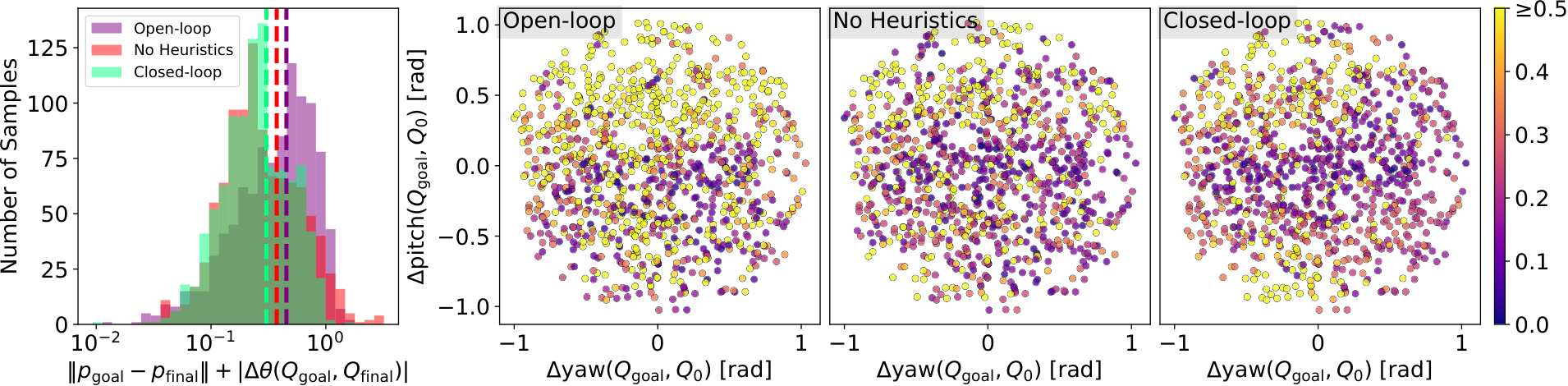
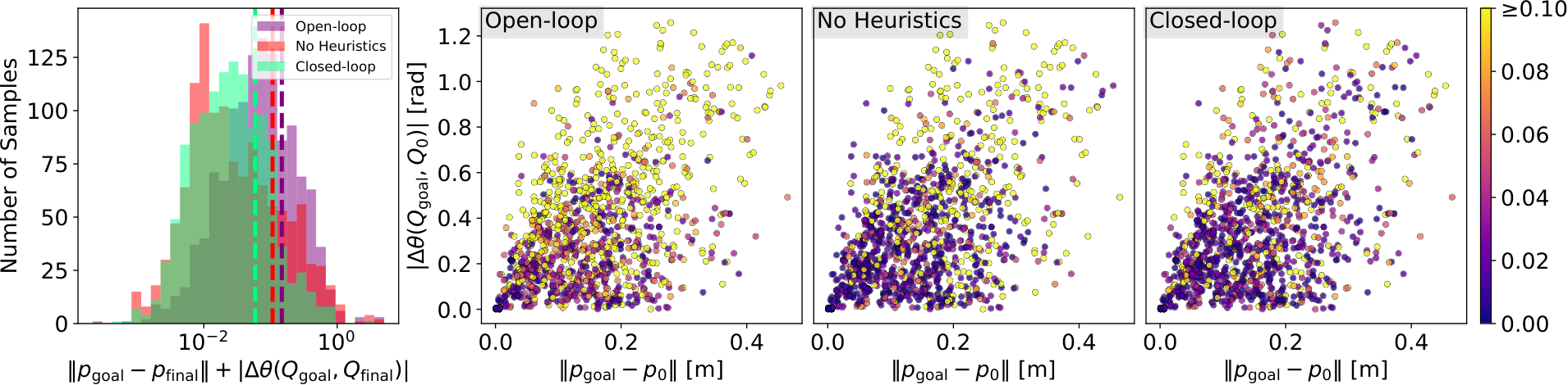
Figure 12: Results for running the five variants of Algorithm 3, namely open-loop, no heuristics, close-loop, and closed-loop with CTR and ETR, on the pairs of goals and initial conditions generated in Section 5.1.1. All figure elements follow the same definitions used in Figure 11.

6.2 Experiment Setup

Ablations compare feedback, open-loop execution, less frequent contact projection, and the three trust regions. Drake and hardware are carefully matched in geometry, gains, friction, and inertia. Object pose comes from OptiTrack; the cube uses embedded active markers and a non-penetration inverse-kinematics correction. The method is state based and assumes this reliable external pose measurement. See Castro et al. (2023) for the cited foundation.

6.3 Results & Discussion

The evaluation separates gains from feedback, renewed contact initialization, and trust-region constraints. Table 6 reports physical-unit errors for both simulated and hardware trials, while the plots expose the different failure distributions.

IiwaBimanual AllegroHand
Trans. [m] Rot. [rad] Trans. [m] Rot. [rad]
Open-loop Sim 0.033 0.115 0.011 0.443
(0.152) (0.191) (0.007) (0.286)
No-Heuristics Sim 0.041 0.066 0.015 0.358
(0.156) (0.153) (0.017) (0.335)
Closed-loop Sim 0.020 0.039 0.014 0.290
with R-CTR (0.065) (0.079) (0.009) (0.197)
Closed-loop Sim 0.040 0.076 0.013 0.349
with ETR (0.167) (0.214) (0.010) (0.267)
Closed-loop Sim 0.031 0.051 0.013 0.289
with CTR (0.122) (0.164) (0.010) (0.211)
Open-loop HW 0.016 0.056 0.014 0.323
(0.019) (0.064) (0.007) (0.256)
Closed-loop HW 0.013 0.024 0.018 0.258
(0.016) (0.038) (0.011) (0.215)
Table 6: Translation and rotation errors for simulation (Sim) and hardware (HW) experiments. Each cell displays the mean (standard deviation).

6.3.1 Closed-loop vs. Open-loop

Replanning substantially improves both systems compared with executing the entire plan without object-state feedback. This demonstrates the value of correction despite an imperfect planning model.

6.3.2 AllegroHand vs. IiwaBimanual

Allegro errors are larger because lifting the cube makes slipping costly: a slip can return it to the palm and erase progress. The tabletop supports the bimanual object, so slipping usually only delays movement. The orientation-dependent results reflect this difference in physical support.

6.3.3 Closed-loop vs. No Heuristics

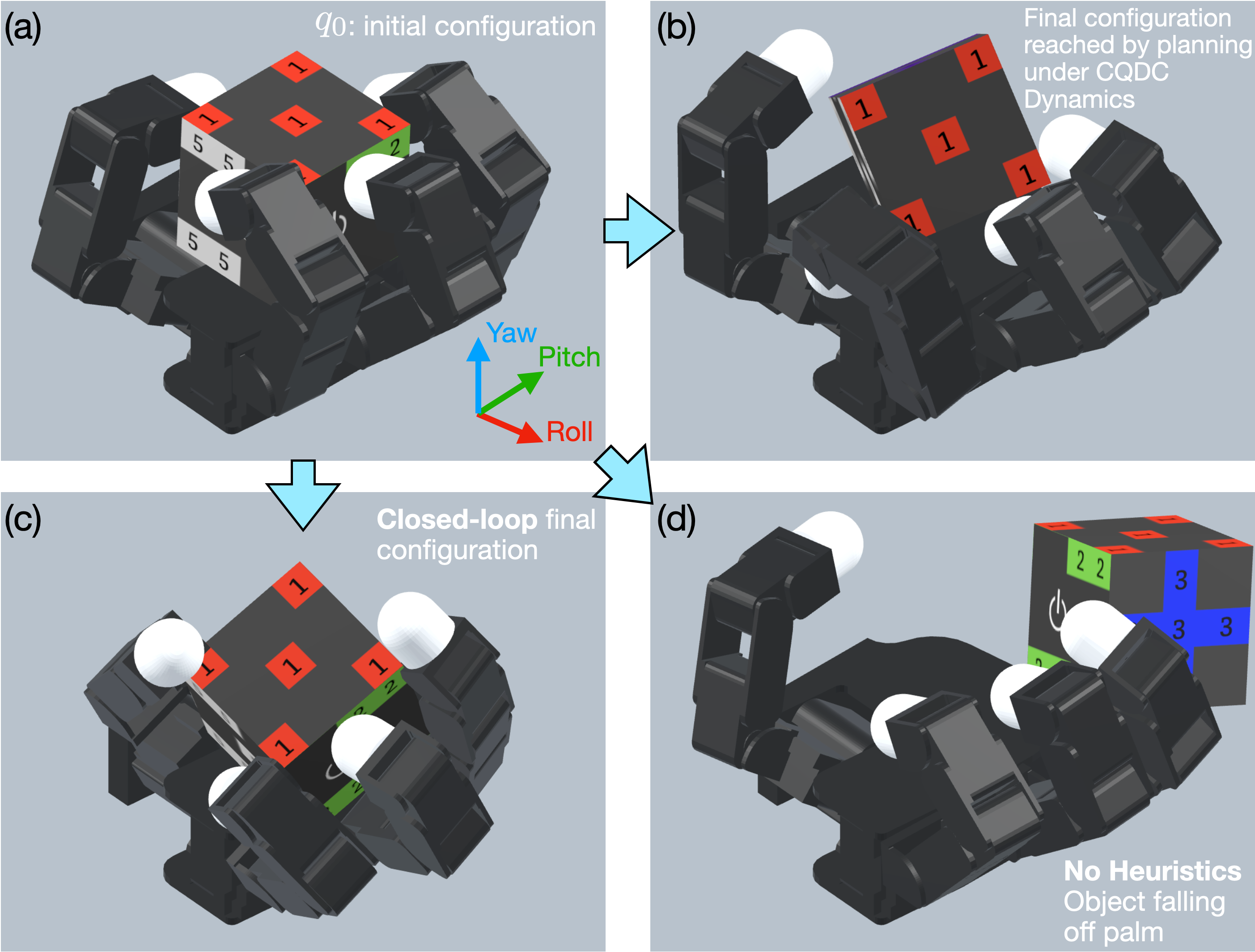
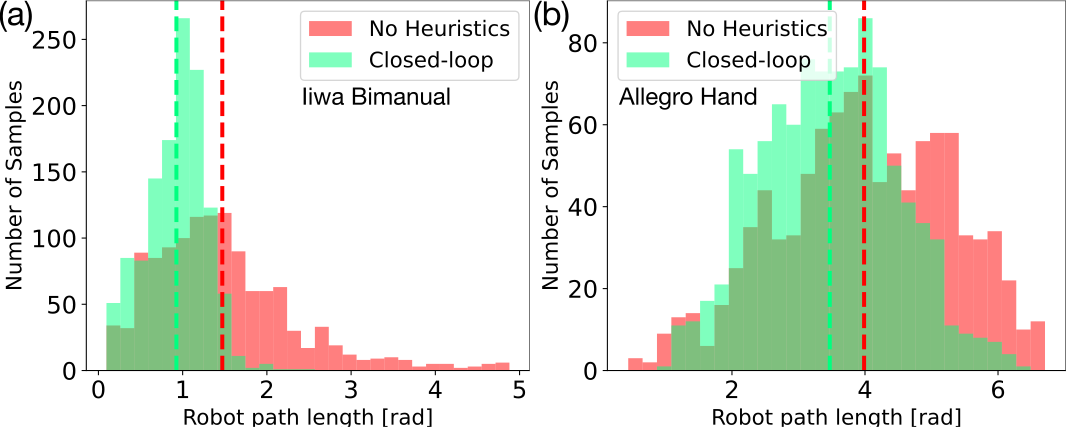
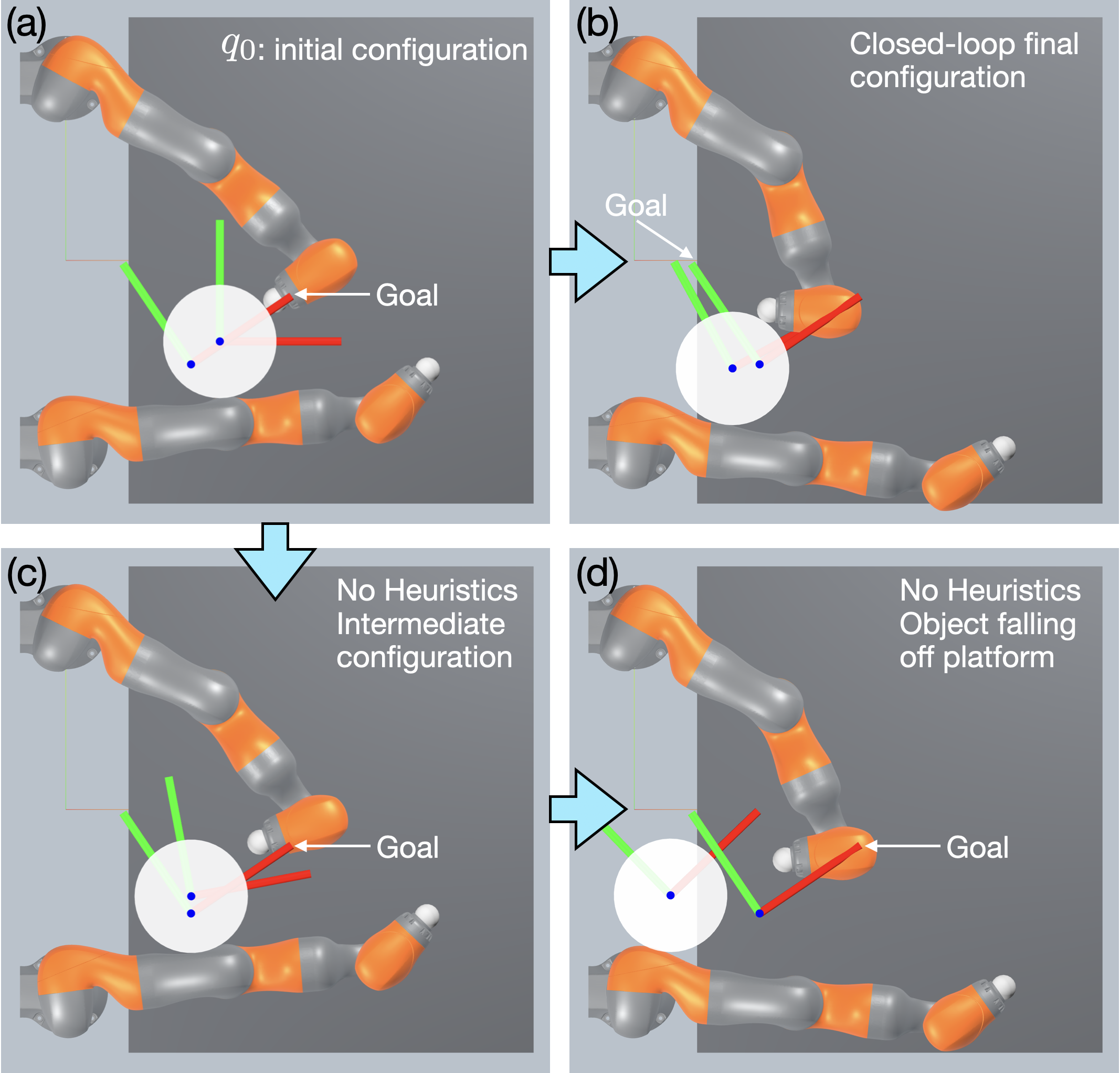
Frequent contact-seeking initialization reduces extreme errors and shortens robot paths more clearly than it changes mean error. It reduces large recovery motions after losing contact and helps prevent the object falling from its support, although contact loss is not eliminated.

Equation 39
Robot Path Length=∫0tfinal‖q˙a​(t)‖2​𝑑t,\text{Robot Path Length}\;=\;\int_{0}^{t_{\text{final}}}\|\dot{q}^{\mathrm{a}}(t)\|_{2}\,\mathrm{d}t, (39)

6.3.4 R-CTR vs. ETR/CTR

The relaxed region gives the best reported combined-error distributions, with a clearer advantage on the bimanual task. Full and relaxed contact regions are close on Allegro, and both improve on ellipsoidal constraints. Individual translation and rotation columns do not all rank the methods identically, so the combined score should not be read as dominance on every metric.

6.3.5 Hardware Experiments

Hardware evaluation uses 50 spatially distributed initial-state/goal pairs per system. Mean errors resemble the matched second-order simulation, supporting transfer under the carefully calibrated conditions. This is 100 local hardware trials across two platforms, distinct from the later long roadmap traversal.
Original figure
Figure 13: Robot Path Length Comparison between the Closed-loop and No Heuristics variants of Algorithm 3. Dotted vertical lines indicate the mean values of each color-coded sample set.
Refer to caption
Figure 14: Failures of Algorithm 3 on Iiwabimanual. The dark gray box represents the table top which supports the bucket. The light gray area represents empty space.
Refer to caption
Figure 15: Failures of Algorithm 3 on AllegroHand.

7 Generating Goal-conditioned Contact Configurations

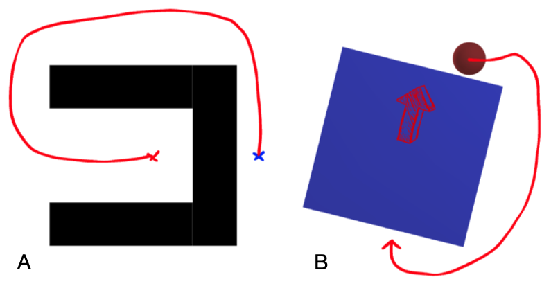
Global manipulation can require moving away from the goal or repositioning before making progress. The paper therefore searches for advantageous contact configurations, then links them with local control. It assumes the object can remain stable while collision-free motion repositions the fully actuated robot; that assumption is essential to separating grasp selection from transit planning.
Refer to caption
Figure 16: Difficult cases for greedy finite-horizon MPC that require long-horizon exploration capabilities. A. A classical example for path-finding where the robot needs to go from the red X to the blue X. Note that the robot needs go back first, momentarily suffering an increase in Euclidean distance, before it can proceed towards the blue X and reach the goal. B. A similar planar-pushing example in manipulation, where the goal is to push the box upwards. From this configuration, the agent must break contact and travel all around to the back of the box, causing no effect in making progress towards the goal in terms of box movement, in order to push the box up.

7.1 Problem Specification

For fixed current and desired object poses, optimize the robot configuration subject to joint limits and non-penetration. Its score combines predicted finite-horizon control cost with a preference for disturbance-resistant contact geometry.

Equations 40a–40c
minqa\displaystyle\min_{q^{\mathrm{a}}}\;\; C⁡(qa,qo,qgo)\displaystyle C(q^{\mathrm{a}};{q^{\mathrm{o}}},q^{\mathrm{o}}_{g}) (40a)
s.t.   ql​ba≤qa≤qu​ba,\displaystyle q_{lb}^{\mathrm{a}}\leq q^{\mathrm{a}}\leq q_{ub}^{\mathrm{a}}, (40b)
ϕi​(qa,qo)≥0∀i,\displaystyle\phi_{i}(q^{\mathrm{a}},q^{\mathrm{o}})\geq 0\quad\forall i, (40c)

7.1.1 Finite-Horizon Value Function of the MPC Policy

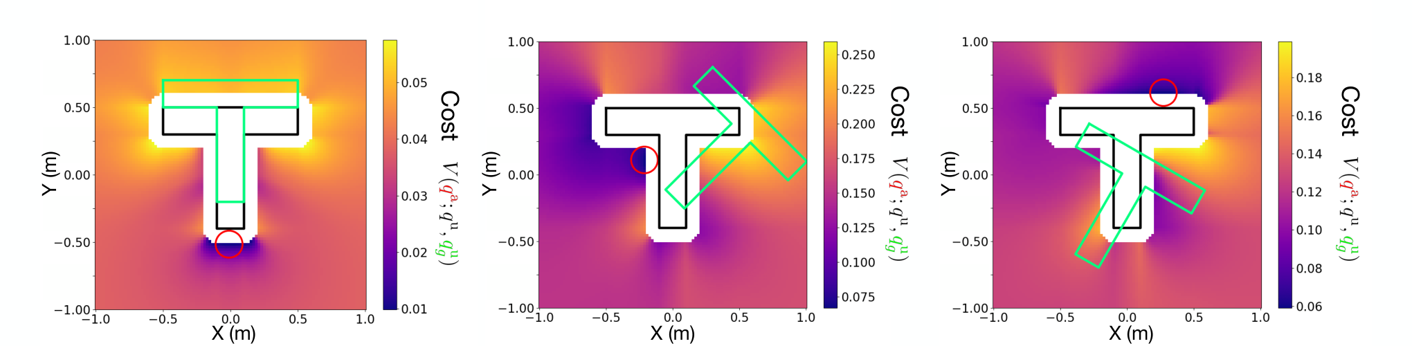
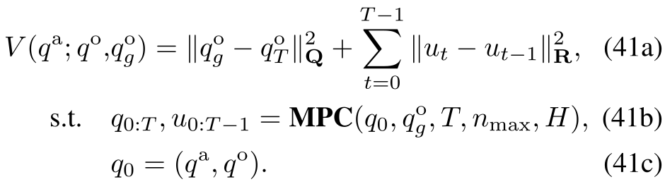
A candidate grasp is scored by rolling out MPC and evaluating its accumulated objective, with no penalty on desired robot joint positions. Even a simple pushing example yields a multimodal landscape, motivating sampled global search rather than relying on a single local descent.

Equations 41a–41c
Original PDF equation 41 with complete source notation and layout.
Refer to caption
Figure 17: Visualization of the landscape of (41) for the planar pusher-T example inspired by Chi et al. (2024). The black T corresponds to the current object configuration qo{q^{\mathrm{o}}}, and the green T the goal object configuration qgoq^{\mathrm{o}}_{g}. The landscape corresponds to the position of the round pusher qaq^{\mathrm{a}}, colored with the cost function V⁡(qa,qo,qgo)V({q^{\mathrm{a}}};{q^{\mathrm{o}}},q^{\mathrm{o}}_{g}). The red pusher configuration corresponds to the global optima of the landscape.

7.1.2 Robustness Regularizer

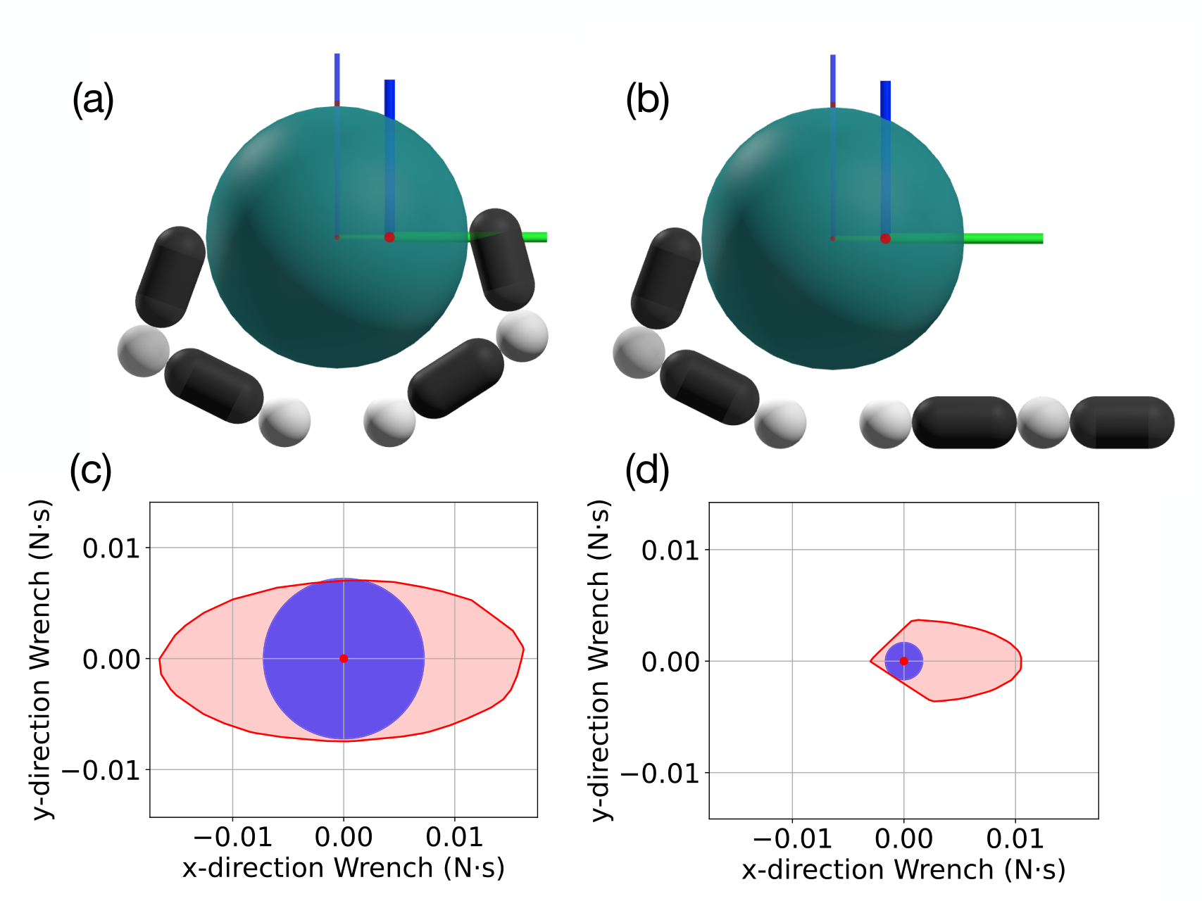
The robustness term rewards an origin-centered inscribed sphere in an approximate wrench set, representing resistance to disturbances from arbitrary directions. The set is estimated by sampling the relaxed action region, rejecting infeasible forces, and taking a convex hull. This is a sampled, local model-based metric; it is not a hardware disturbance guarantee. See Ferrari and Canny (1992) for the cited foundation.

Equations 42a–43b
r⁡(qa,qo)≔minv\displaystyle r({q^{\mathrm{a}}},{q^{\mathrm{o}}})\coloneqq\min_{v} maxr∈ℝ⁡r\displaystyle\max_{r\in\mathbb{R}}\;r (42a)
s.t.  ‖v‖=1\displaystyle\|v\|=1 (42b)
r​v∈𝒲𝚺,κ𝒜​(q¯=(qa,qo),u¯=qa).\displaystyle rv\in\mathcal{W}_{\mathbf{\Sigma},\kappa}^{\mathcal{A}}(\bar{q}=({q^{\mathrm{a}}},{q^{\mathrm{o}}}),\bar{u}=q^{\mathrm{a}}). (42c)
maxr≥0\displaystyle\max_{r\geq 0}\; r\displaystyle r (43a)
s.t.  ‖ai‖2​r+bi≤0∀i.\displaystyle\|a_{i}\|_{2}r+b_{i}\leq 0\quad\forall i. (43b)

7.1.3 Total Cost

The total objective subtracts a weighted squared robustness radius from the MPC cost. The weight trades short-term goal progress against contact configurations that can oppose a broader set of disturbances.

Equation 44
C⁡(qa,qo,qgo)=V⁡(qa,qo,qgo)−α​r​(qa,qo)2,C({q^{\mathrm{a}}};{q^{\mathrm{o}}},q^{\mathrm{o}}_{g})=V({q^{\mathrm{a}}};{q^{\mathrm{o}}},q^{\mathrm{o}}_{g})-\alpha r({q^{\mathrm{a}}};{q^{\mathrm{o}}})^{2}, (44)
Refer to caption
Figure 18: Top Row: Comparison of two configurations (a) and (b) for the 2D planar hand system in Figure 5. Although both configurations are advantageous for moving the object to the goal, they share the same MPC value function cost (Table 7). Bottom Row: Plot of the wrench set (illustrated in red) and the maximum inscribed sphere (blue), where (c) corresponds to configuration (a) and (d) corresponds to (b). Note that configuration (a) has a much larger inscribed sphere due to the anti-podal grasp.
Configuration (a) (b)
MPC value function VV 2.82×10−42.82\times 10^{-4} 2.16×10−42.16\times 10^{-4}
Max inscribed sphere radius 7.12×10−37.12\times 10^{-3} 1.68×10−31.68\times 10^{-3}
Table 7: Comparison of MPC value function cost and maximum inscribed sphere radius for two configurations in Figure 18.

7.2 Solving ( 40 ) by Sampling-based Optimization

Rejection sampling and best-candidate selection handle the nonconvex grasp objective without differentiating through the whole rollout. Direct sampling is inefficient in high-dimensional joint space, so Allegro uses a reduced fingertip model and projection heuristics described in the appendix.
Refer to caption
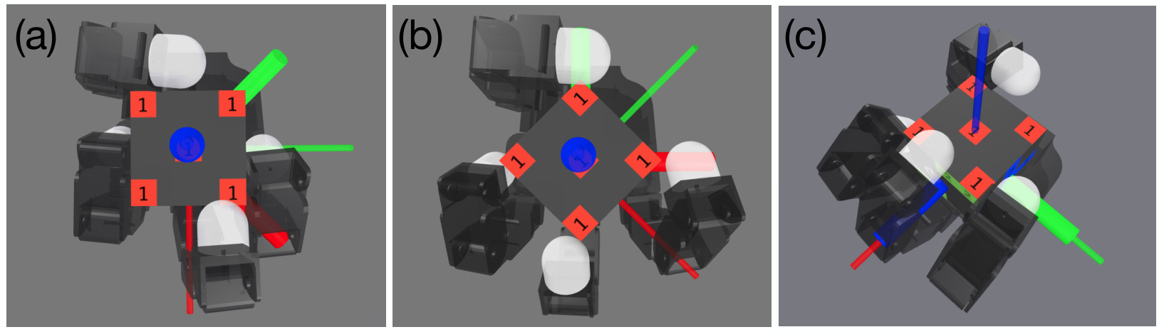
Figure 19: Initial actuator configurations found by our method for (a) yaw 0∘0^{\circ} to 45∘45^{\circ}, (b) yaw 45∘45^{\circ} to 90∘90^{\circ}, and (c) pitch 0∘0^{\circ} to 90∘90^{\circ}. The initial configuration of the cube is marked with a long and thin triad, while the goal configuration of the cube a short and thick triad.
Task Position [mm] Rotation [mrad] Time [s]
Yaw 0∘→45∘0^{\circ}\!\to\!45^{\circ} 12.05 (3.49) 32.41 (27.14) 57.83 (2.08)
Yaw 45∘→90∘45^{\circ}\!\to\!90^{\circ} 9.85 (10.88) 15.72 (21.08) 57.28 (0.72)
Pitch 0∘→90∘0^{\circ}\!\to\!90^{\circ} 21.42 (8.91) 32.12 (32.03) 57.84 (0.73)
Table 8: Performance of our algorithm for finding initial actuator configurations. Results are obtained with 1010 repeated runs. Each run is optimized using 10001000 samples. Each cell displays the mean (standard deviation).

7.3 Results

Across three selected cube rotations, ten repeated searches using 1,000 reduced-model samples each find configurations with errors around 10 mm and 30 mrad. Fewer samples may reduce cost but increase variability. Some opposite-pitch and roll motions remain physically difficult; this is not arbitrary-pose grasp synthesis.

8 Global Planning with Roadmaps

A reusable roadmap composes useful grasp configurations and their local transition plans. Offline construction searches for connections; online inference connects the requested endpoints and searches the resulting graph. See Choset et al. (2005) for the cited foundation.

8.1 Roadmap Construction

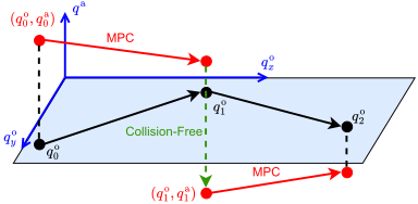
Each edge first moves the object with MPC, then repositions the hand with collision-free planning while the object stays fixed. Cube symmetry expands a few grasps and three basic rotations into 24 equivalent orientations, keeping this specialized roadmap below ten minutes of offline construction. On hardware, a random walk completed 150 consecutive transitions before the hand overheated. The authors attribute reliability partly to symmetry and grasps that cage and recenter the cube.
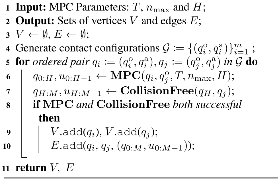
Algorithm 4 Roadmap Construction
Original PDF algorithm 4 with complete source notation and layout.
Original figure
Figure 20: Illustration of roadmap construction described by Algorithm 4. The vertical axis represents the actuator configuration qa{q^{\mathrm{a}}}, while the horizontal plane the space of object configurations qo{q^{\mathrm{o}}}. To connect the vertices q0:=(q0o,q0a)q_{0}:=(q^{\mathrm{o}}_{0},q^{\mathrm{a}}_{0}) and q1:=(q1o,q1a)q_{1}:=(q^{\mathrm{o}}_{1},q^{\mathrm{a}}_{1}), we first plan from q0q_{0} to q1oq^{\mathrm{o}}_{1} with MPC, reaching the top red dot. As the top red dot and q1q_{1} share the same object configuration q1oq^{\mathrm{o}}_{1}, we can connect them with a collision free planner.
Refer to caption
Figure 21: A complete path generated by our roadmap-based global planner. The object configuration in each frame is highlighted at the lower-left corner. (a) shows the starting configuration, which in this example is a vertex already in the roadmap. (b) can be reached from (a) with a −90∘-90^{\circ} yaw. (c) has the same object configuration as (b), but the hand has repositioned for a 90∘90^{\circ} pitch. (d) is system configuration after the pitch. (e) shows the system reaching the goal configuration from (d). The path (a)-(d) is part of the roadmap and generated offline. (d)-(e) is generated online using collision-free planning and local MPC.

8.2 Inference on a Roadmap

Online planning connects the start and goal to nearby roadmap vertices, then finds a shortest graph path. The precomputed local transitions are reused, with endpoint connections solved for the new request. Success still depends on those connections being feasible.

8.3 Limitations

The roadmap is specialized to Allegro and a symmetric cube resting in stable palm-supported poses. General shapes require more explicit reachability reasoning, and unstable poses cannot be treated as static during finger repositioning. Finger gaiting or other stability-aware transit strategies would be needed to broaden applicability.

9 Discussion and Conclusion

The discussion separates the demonstrated model-based controller from possible uses in learning, then identifies unresolved contact-model and global-planning limitations.

9.1 Synergies with Learning-based Methods

The planner could complement learned policies by producing demonstrations, recovery trajectories, or useful exploration states. These are proposed interfaces to imitation and reinforcement learning rather than additional learning experiments established here.

9.1.1 Data Synthesis and Augmentation for IL

Potential imitation-learning uses include generating contact-rich demonstrations that are hard to teleoperate and recovering from perturbed demonstrations to enrich training data. Distilling such trajectories into a policy could reduce online planning cost. The discussion motivates this direction; it does not report a trained general policy as an outcome of these experiments. See Yang et al. (2025) for the cited foundation.

9.1.2 Efficient Exploration for RL

Stable roadmap states and successful trajectories could guide reinforcement-learning resets, rewards, or exploration. Prior planner-assisted learning work motivates this idea, but the claim that this roadmap is an efficient exploration distribution remains a hypothesis. See Khandate et al. (2024) for the cited foundation.

9.2 Concluding Remarks and Limitations

Local control succeeds on most sampled reachable goals, and a specialized roadmap extends its range. Remaining gaps include unexplained failures, incomplete understanding of primal versus dual feasibility, loss of contact under second-order dynamics, and dependence on stable symmetric roadmap nodes. Extension to other robots is plausible from supplied models, but may require added balance constraints and careful calibration; it has not been established universally.

Appendix A Appendix

The appendix supplies sensitivity and wrench-set derivations, goal sampling, hyperparameters, reduced-order grasp search, and additional failure/success examples.

A.1 Derivation of ( 15 )

Differentiating stationarity and perturbed complementarity produces the stated action-sensitivity relation. The appendix explicitly warns that this displayed relation alone is not invertible for higher-dimensional friction cones: the appropriate vector cone relation must be differentiated instead. The full matrix-calculus derivation is omitted, so the scalar-cone shortcut should not be implemented as a general friction-cone solver. See Magnus and Neudecker (2019) for the cited foundation.

Equations 45a–46b
𝐏​q++b−∑i𝐉i⊤​λi\displaystyle\mathbf{P}q_{+}+b-\sum_{i}\mathbf{J}_{i}^{\top}\lambda_{i} =0,\displaystyle=0, (45a)
νi⊤​λi\displaystyle\nu^{\top}_{i}\lambda_{i} =2​κ−1,∀i.\displaystyle=2\kappa^{-1},\quad\forall i. (45b)
𝐏​∂q+∂u+∂b∂u−∑i𝐉i⊤​∂λi∂u\displaystyle\mathbf{P}\frac{\partial q_{+}}{\partial u}+\frac{\partial b}{\partial u}-\sum_{i}\mathbf{J}_{i}^{\top}\frac{\partial\lambda_{i}}{\partial u} =0\displaystyle=0 (46a)
(𝐉i​∂q+∂u)⊤​λi+∂λi∂u⊤​(𝐉i​q++ci)\displaystyle\left(\mathbf{J}_{i}\frac{\partial q_{+}}{\partial u}\right)^{\top}\lambda_{i}+\frac{\partial\lambda_{i}}{\partial u}^{\top}(\mathbf{J}_{i}q_{+}+c_{i}) =0∀i\displaystyle=0\quad\forall i (46b)

A.2 Proof of Lemma 2

The equivalence proof uses the earlier first-order force-balance lemma: joint linear predictions of contact impulse and object displacement satisfy the same quasidynamic balance. It identifies the resulting motion construction under the stated local assumptions, rather than proving exact reachability for nonlinear physical contact. The appendix uses a shared actuator perturbation across contacts; its force/impulse and time-step conventions differ from the preceding wrench formulas, so the equations are preserved rather than silently normalized.

Equations 47a–52
𝒲(q¯,u¯)={w\displaystyle\mathcal{W}(\bar{q},\bar{u})=\{w |w=∑i𝐉oi⊤λ^i\displaystyle|w=\sum_{i}\mathbf{J}_{\mathrm{o}_{i}}^{\top}\hat{\lambda}_{i} (47a)
λ^i\displaystyle\hat{\lambda}_{i} =𝐃i​δ​u+λ⁡(q¯,u¯)\displaystyle=\mathbf{D}_{i}\delta u+\lambda(\bar{q},\bar{u}) (47b)
δ​u⊤​𝚺​δ​u\displaystyle\delta u^{\top}\mathbf{\Sigma}\delta u ≤1\displaystyle\leq 1 (47c)
λ^i\displaystyle\hat{\lambda}_{i} ∈𝒦i⋆}.\displaystyle\in\mathcal{K}^{\star}_{i}\}. (47d)
ℳΣ,κ𝒜,o​(q¯,u¯)≔{𝐁o​δ​u+fo​(q¯,u¯)|δ​u∈𝒮~Σ,κ𝒜​(q¯,u¯)}\mathcal{M}_{\Sigma,\kappa}^{\mathcal{A},\mathrm{o}}(\bar{q},\bar{u})\coloneqq\{\mathbf{B}^{\mathrm{o}}\delta u+f^{\mathrm{o}}(\bar{q},\bar{u})|\delta u\in\tilde{\mathcal{S}}^{\mathcal{A}}_{\Sigma,\kappa}(\bar{q},\bar{u})\} (48)
{q+o|ϵh𝐌o(q¯)(q+o−q¯o)=hτo+w,w∈𝒲}.\{{q^{\mathrm{o}}_{\texttt{+}}}|\frac{\epsilon}{h}\mathbf{M}_{\mathrm{o}}(\bar{q})(q^{\mathrm{o}}_{+}-\bar{q}^{\mathrm{o}})=h\tau^{\mathrm{o}}+w,w\in\mathcal{W}\}. (49)
q^+o\displaystyle\hat{q}_{+}^{\mathrm{o}} =𝐁o​δ​u+fo​(q¯,u¯),\displaystyle=\mathbf{B}^{\mathrm{o}}\delta u+f^{\mathrm{o}}(\bar{q},\bar{u}), (50)
λ^i\displaystyle\hat{\lambda}_{i} =𝐃i​δ​u+λi​(q¯,u¯),\displaystyle=\mathbf{D}_{i}\delta u+\lambda_{i}(\bar{q},\bar{u}), (51)
εh​𝐌o​(q^+o−q¯o)=h​τo+∑i𝐉oi⊤​λ^i.\displaystyle\frac{\varepsilon}{h}\mathbf{M}_{\mathrm{o}}\left(\hat{q}_{+}^{\mathrm{o}}-\bar{q}^{\mathrm{o}}\right)=h\tau^{\mathrm{o}}+\sum_{i}\mathbf{J}_{\mathrm{o}_{i}}^{\top}\hat{\lambda}_{i}. (52)

A.3 Goal Generation for Local MPC

Bimanual goals come from the boundary of a large local action-only motion set after sampling contacts and solving inverse kinematics; Allegro targets differ by about 60 degrees. The actual datasets contain 1,233 and 1,000 pairs respectively. Table 9 gives the no-motion baseline errors, clarifying the sampled goals’ scale and selection bias toward local reachability.

IiwaBimanual AllegroHand
Mean ∥pgoal−p0∥\lVert p_{\text{goal}}-p_{0}\rVert [mm] 152 16
Mean |Δ​θ​(Qgoal,Q0)|\lvert\Delta\theta(Q_{\text{goal}},Q_{0})\rvert [mrad] 356 788
Table 9: Mean translation and rotation differences for pairs of initial and goal object states generated in this section.

A.4 Effect of Planning Horizon for Local MPC

For the sampled bimanual goals, increasing the internal planning horizon from one to five barely changes final error. The proposed explanation is that quadratic goal distance approximates the cost-to-go well in this regime. This does not establish one-step optimality generally, especially for the nonlocal tasks motivating the roadmap.

T=1T=1 T=2T=2 T=3T=3 T=4T=4 T=5T=5
Translation [mm] 2.02 1.99 1.64 2.11 2.10
(3.10) (4.38) (3.14) (3.79) (3.17)
Rotation [mrad] 2.72 3.51 3.25 4.13 5.03
(0.75) (1.18) (2.87) (1.41) (2.82)
Table 10: Translation and rotation Errors for IiwaBimanual under different planning horizon TT. The first row is the mean; the second row (numbers in brackets) is the standard deviation.

A.5 Hyperparameters for Local MPC

Object error and action regularization drive the cost; robot goal-coordinate weights are zero. Smoothing and time step trade informative gradients against model fidelity and execution length. Distant contact pairs are pruned using a conservative signed-distance threshold. More principled bounds could reduce the number of constraints further.

IiwaBimanual AllegroHand
𝐐o\mathbf{Q}_{\mathrm{o}} Rotation 0.1​𝐈10.1\mathbf{I}_{1} 𝐈3\mathbf{I}_{3}
Translation 𝐈2\mathbf{I}_{2} 5​𝐈35\mathbf{I}_{3}
𝐑\mathbf{R} 0.01​𝐈60.01\mathbf{I}_{6} 0.01​𝐈160.01\mathbf{I}_{16}
κ\kappa 10410^{4} 10410^{4}
hh [s] 0.020.02 0.050.05
ϕ\phi-threshold [m] 0.2 0.05
Table 11: Additional hyperparameters for MPC, used by both Algorithm 2 and Algorithm 3.

A.6 Hyperparameters for 2nd-order Dynamics Stabilization

Second-order experiments tune rollout length and replanning count differently for tabletop and in-hand manipulation. The reported sweep shows almost no correlation between chunk length and final error. The robot pauses during replanning, so the chosen lengths also balance computation pauses against feedback frequency.

NN (Number of re-plans) HH (MPC rollout horizon)
System open-loop closed-loop open-loop closed-loop
IiwaBimanual 1 Variable 25 5
AllegroHand 1 5 50 10
Table 12: Hyperparameters for the MPC in Algorithm 3. No Heuristics and Closed-loop share the same parameters.
Original figure
Figure 22: Analysis of closed-loop tracking error as a function of the rollout horizon HH. Performance is largely insensitive to this hyperparameter. For IiwaBimanual, there is a negligible correlation between HH and tracking error (r=0.00082r=0.00082). A minor negative correlation is observed for AllegroHand (r=−0.059r=-0.059), which we attribute to violations of the quasi-dynamic assumption. Error bars represent 0.1​σ0.1\sigma.
Refer to caption
Figure 23: (a) Visualization of the reduced-order system for the Allegro in Section A.7.1, which consists of four spheres. (b) Visualization of the IK result on the optimized solution, mapping the reduced-order system to the full system.

A.7 Heuristics for Generating Allegro Contact Configurations

Allegro grasp search first optimizes a simplified fingertip representation and then maps it to joint configurations. Sampling is biased toward actual surface contact to avoid ineffective separated fingertips.

A.7.1 A Reduced-Order Model

Four independently moving bounded spheres approximate the fingertips. Iterative quadratic-program inverse kinematics matches their optimized positions with the real hand while enforcing linearized non-penetration. This reduces search dimensionality but relies on the mapping being achievable with the hand’s kinematics.

Equations 53a–53d
minδ​q,p+,k\displaystyle\min_{\delta q,p_{+,k}}\;\; ∑k‖p+,k−pdes,k‖2\displaystyle\sum_{k}\|p_{+,k}-p_{\text{des},k}\|^{2} (53a)
s.t.   p+,k=pk+∂pk∂q​δ​q\displaystyle p_{+,k}=p_{k}+\frac{\partial{p_{k}}}{\partial q}\delta q (53b)
𝐉ni​δ​q+ϕi≥0\displaystyle\mathbf{J}_{n_{i}}\delta q+\phi_{i}\geq 0 (53c)
−ε​𝟏≤δ​q≤ε​𝟏,\displaystyle-\varepsilon\mathbf{1}\leq\delta q\leq\varepsilon\mathbf{1}, (53d)
Refer to caption
(a) A goal which MPC with R-CTR successfully reached but the ETR baseline failed to reach. Note the initial contact points in frame (1) do not form a force-closure grasp. Without the dual feasibility constraint, ETR does not recognize the unilateral-ness of the initial contact configuration and fails catastrophically.
Refer to caption
(b) A goal which both R-CTR and ETR-based MPC successfully reached. Note how the initial contact points form a nice anti-podal grasp on the cylinder.
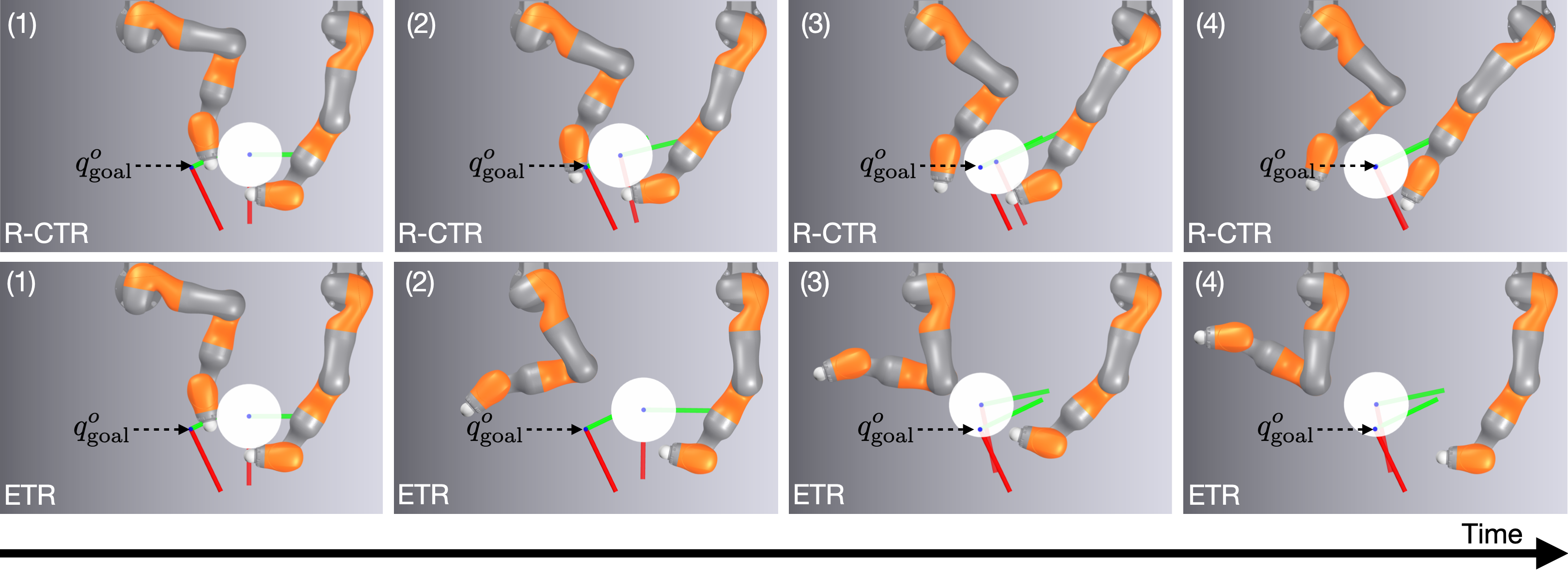
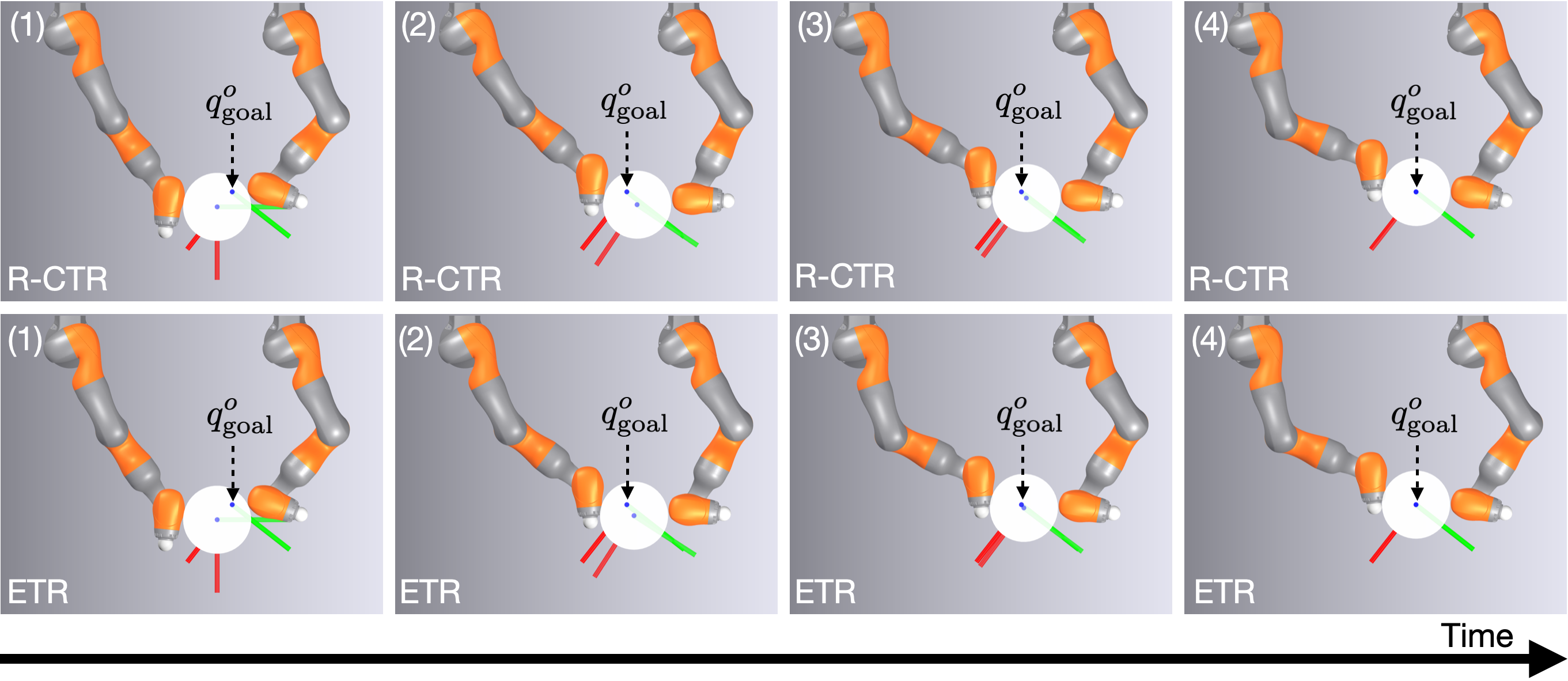
Figure 24: Example trajectories for IiwaBimanual from running local MPC (Algorithm 2) to reach the goals generated in Section 5.1.1. While R-CTR-based MPC reaches both goals successfully, ETR-based MPC fails in (a) but succeeds in (b).

A.7.2 Contact Sampling Distribution

Sampled sphere positions are projected onto the nearest cube surface. This concentrates candidates on contact configurations and increases the estimated robustness relative to unconstrained volume sampling.

A.8 Local MPC Examples

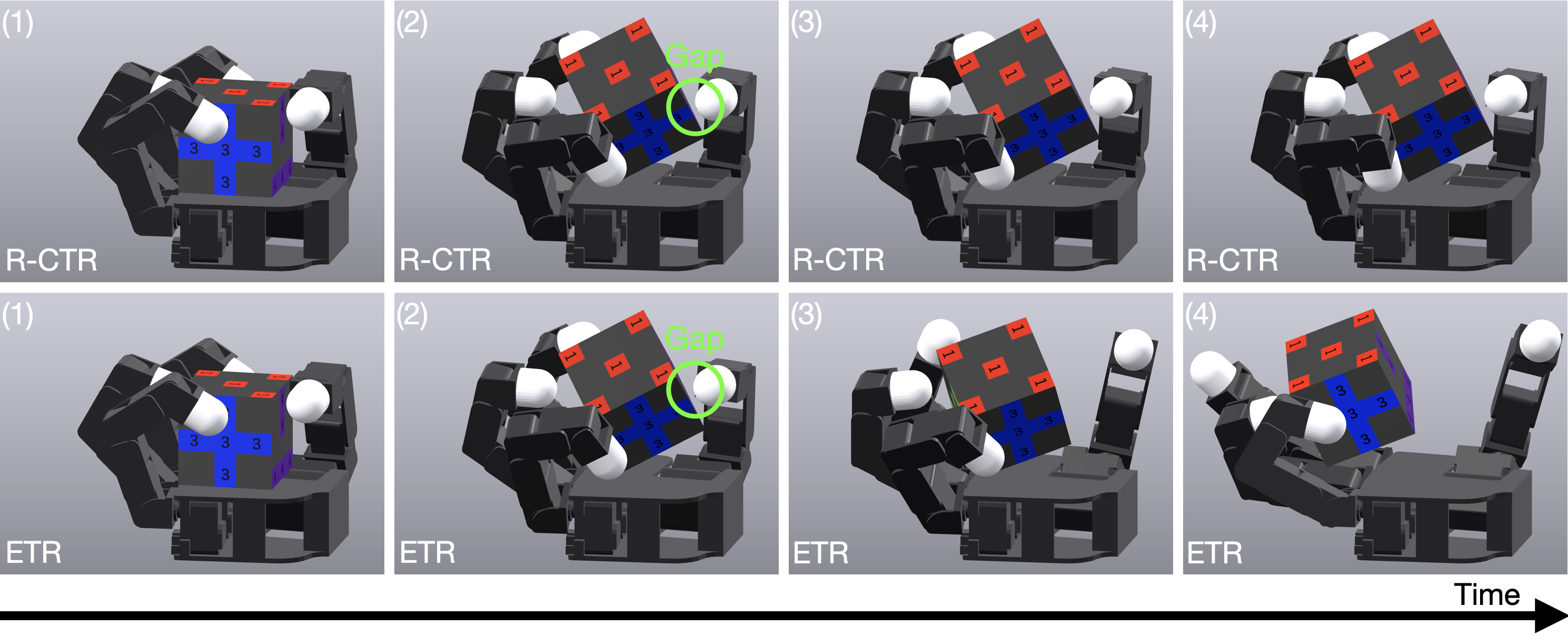
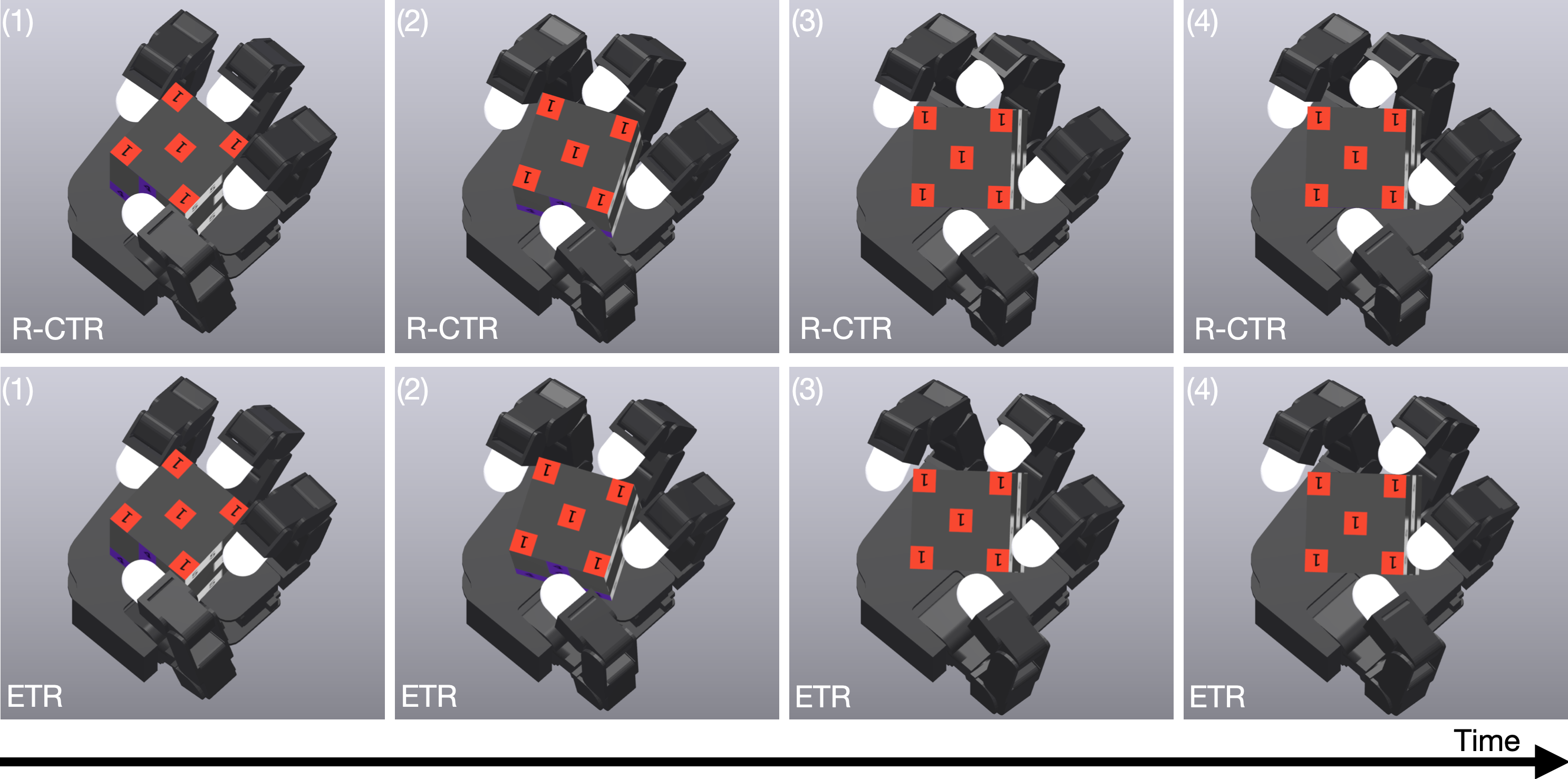
The additional trajectories contrast unilateral configurations, where ellipsoidal control can command fictitious pulling and fail, with stable force-closure grasps where both methods succeed. These examples support the mechanism attributed to dual feasibility while showing why its benefit varies with the initial contact geometry.
Refer to caption
(a) A goal which MPC with R-CTR successfully reached but the ETR baseline failed to reach. The failure begins in frame (2), where a small gap appears between the thumb and the cube. Without the dual feasibility constraint, the ETR-based MPC incorrectly calculates that moving the thumb away from the object will reduce tracking error, leading to a catastrophic failure.
Refer to caption
(b) A goal which both R-CTR and ETR-based MPC successfully reached. Note how the fingers form a nice closure grasp on the cube.
Figure 25: Example trajectories for AllegroHand from running local MPC (Algorithm 2) to reach the goals generated in Section 5.1.1. While R-CTR-based MPC reaches both goals successfully, ETR-based MPC fails in (a) but succeeds in (b).
Concept demonstration

Open image ↗