At a glance
The paper relaxes optimal control with jointly optimized trajectories and discretization time steps into a semidefinite program. A selective, time-scaled lifting captures the relevant polynomial products without constructing a full second-order moment matrix. Sparse variants reduce matrix size, and a graph of convex sets extends the formulation to piecewise-affine mode sequences. Experiments show useful lower bounds and initializations, but exactness is empirical rather than guaranteed; dynamically feasible trajectories are recovered with nonlinear refinement.
I Introduction
Variable time steps make even discretized linear dynamics bilinear in state, control, and time. Alternating optimization or direct collocation can find local solutions, while mixed-integer mode scheduling can become expensive when modes are assigned at every time step. The proposed time-flexible relaxation exploits the structure of these products and embeds mode-level subproblems in a graph. Its contribution is a compact relaxation of a discretized model, not a general proof of globally optimal continuous-time robot control.
Equation 1
| (1) |
II Preliminaries on Semidefinite Relaxation
A standard semidefinite relaxation [35] lifts quadratic products into a positive semidefinite matrix and drops the rank-one constraint. The relaxed optimum is a lower bound on the original minimization problem. A rank-one solution can recover an exact original solution; otherwise feasibility and optimality require additional analysis or recovery. This distinction remains central when the paper combines relaxation with nonlinear trajectory refinement.
Equations 2a–3f
| (2a) | ||||
| (2b) | ||||
| (2c) | ||||
| (2d) | ||||
| (3a) | ||||
| (3b) | ||||
| (3c) | ||||
| (3d) | ||||
| (3e) | ||||
| (3f) | ||||
III Problem Statement
The decision variables are a fixed-length sequence of states and controls plus a positive common time step. States and inputs lie in prescribed polytopes, with fixed start and goal states. The objective combines total duration with time-weighted quadratic state and input penalties. Euler-discretized dynamics and the chosen horizon define the optimization model; their discretization error is separate from the semidefinite relaxation gap.
Equations 4a–4d
| (4a) | ||||
| subject to | (4b) | |||
| (4c) | ||||
| (4d) | ||||
IV Convex Relaxation with Time Scaling
The method first handles linear time-invariant dynamics, then fixed piecewise-affine mode sequences, and finally mode selection. Its main design choice is which time–trajectory products to lift and which redundant original constraints to retain as useful convex restrictions.
IV-A Time-Flexible Relaxation
Collect all trajectory variables in a vector r and lift the vector containing 1, h, r, and hr into a matrix scaled by 1/h. Positivity of h makes this a valid positive semidefinite construction. It retains products needed for both bilinear dynamics and cubic time-weighted costs while omitting the full set of second-order monomials. Multiplying original linear constraints produces additional equalities and inequalities that are redundant before relaxation but tighten the lifted feasible set. The appendix gives the full program.
Equation 5
| (5) |
IV-B Sparse Time-Flexible Relaxation
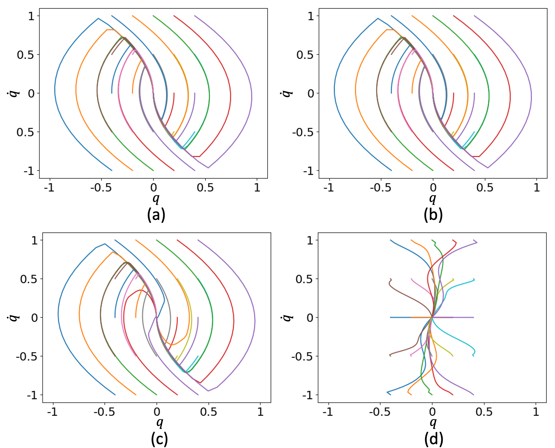
A dense lifted matrix grows with the entire horizon. The sparse formulation instead uses local blocks for adjacent states and the current input, together with consistency constraints for shared states and their lifted products. On the minimum-time double-integrator example, a standard first-order relaxation is loose, while a full second-order matrix would have dimension 4,465 and exhausts memory. Dense TFR uses dimension 186; the reported sparse construction uses 29 matrices of dimension 12 and closely follows the optimal policy. These are example-specific size and tightness results.
Equations 6–7
| (6) |
| (7) |
V Piecewise-Affine Systems with a Fixed Mode Sequence
For a fixed mode sequence, each segment has its own trajectory variables and time step. The formulation relaxes each segment separately, imposes boundary conditions at the endpoints, and couples successive segments through state continuity. This modular structure prepares mode-level graph optimization. The fixed-sequence problem itself has no mode-choice integer variables; the computational benefit concerns the subsequent mode-scheduling formulation.
Equations 8–9e
| (8) |
| (9a) | ||||
| subject to | ||||
| (9b) | ||||
| (9c) | ||||
| (9d) | ||||
| (9e) | ||||
V-A Continuity Constraints with Coupling Matrix
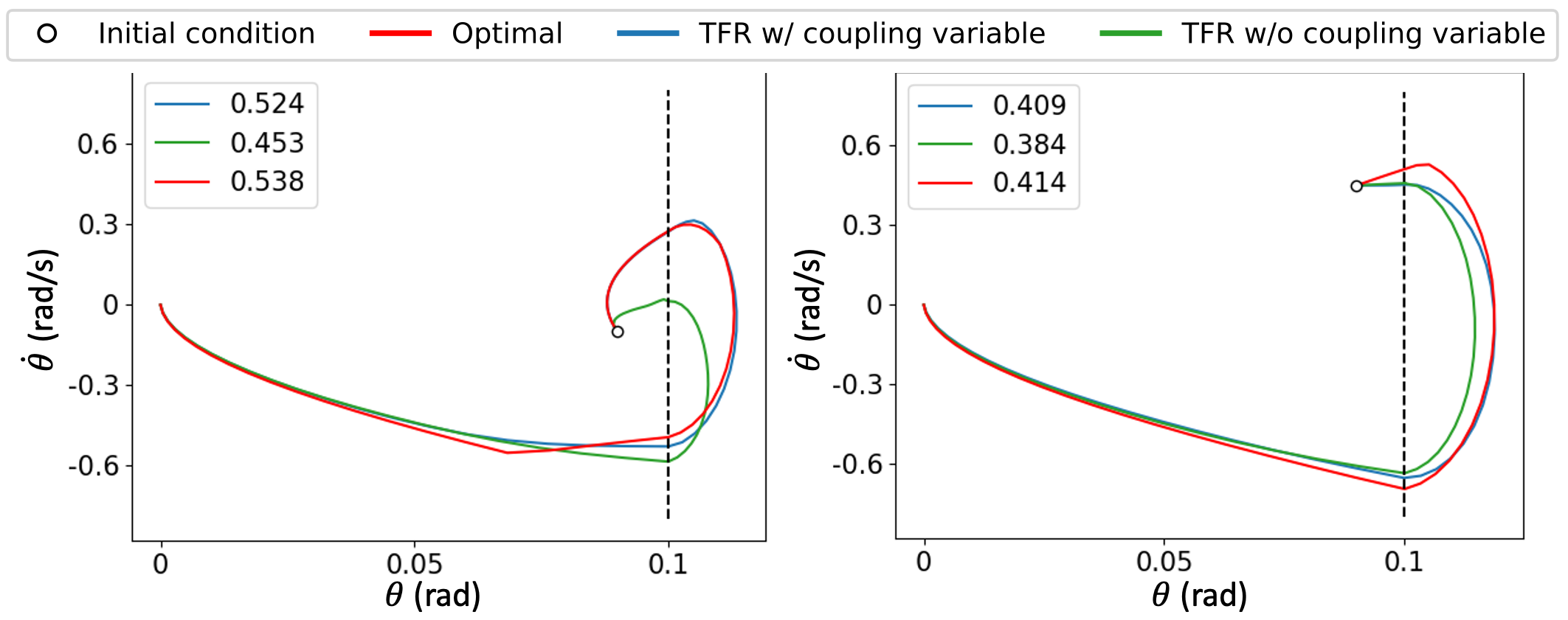
A coupling positive semidefinite matrix contains the shared boundary state together with the time variables from neighboring modes. Matching its entries to the segment matrices aligns both ordinary state moments and time-dependent products, making continuity stronger than simply matching the first-moment state. In the linearized inverted-pendulum example with elastic walls, these constraints tighten the lower bound across the tested initial conditions.
Equations 10
| (10) | ||||
VI Mode Optimization for Piecewise-Affine Systems
Mode sequences become paths through a directed graph, and each mode contributes a convex feasible set describing its relaxed dynamics. The combined formulation relaxes both continuous nonconvex dynamics and discrete path selection.
VI-A Shortest Paths in Graphs of Convex Sets
In a graph of convex sets [27], each vertex carries a continuous variable in a convex set; edge costs and compatibility constraints depend on endpoint variables. Finding the shortest discrete path remains NP-hard. The paper uses a convex relaxation of this graph problem, whose tightness is assessed empirically. A single convex solve therefore returns a relaxed solution, not an unconditional exact solution to arbitrary mode scheduling.
Equations 11a–11d
| (11a) | ||||||
| subject to | (11b) | |||||
| (11c) | ||||||
| (11d) | ||||||
VI-B Spectrahedra as Convex Sets 𝒳 v
The feasible region of each mode’s semidefinite program is a spectrahedron. These regions become graph-vertex sets, and their lifted matrices become the continuous graph variables. Edge constraints impose the mode-to-mode compatibility conditions.
VI-C Optimal Control of PWA Systems with Time Scaling
Solve the combined graph and time-flexible relaxation to obtain a mode sequence and approximate trajectory, then initialize a nonlinear solver on the original bilinear problem for that fixed sequence. This refinement restores dynamical consistency and supplies a feasible upper-bound cost. Comparing it with the relaxed lower bound quantifies the remaining optimality gap; local refinement alone does not prove a global optimum.
VII Additional Experimental Results
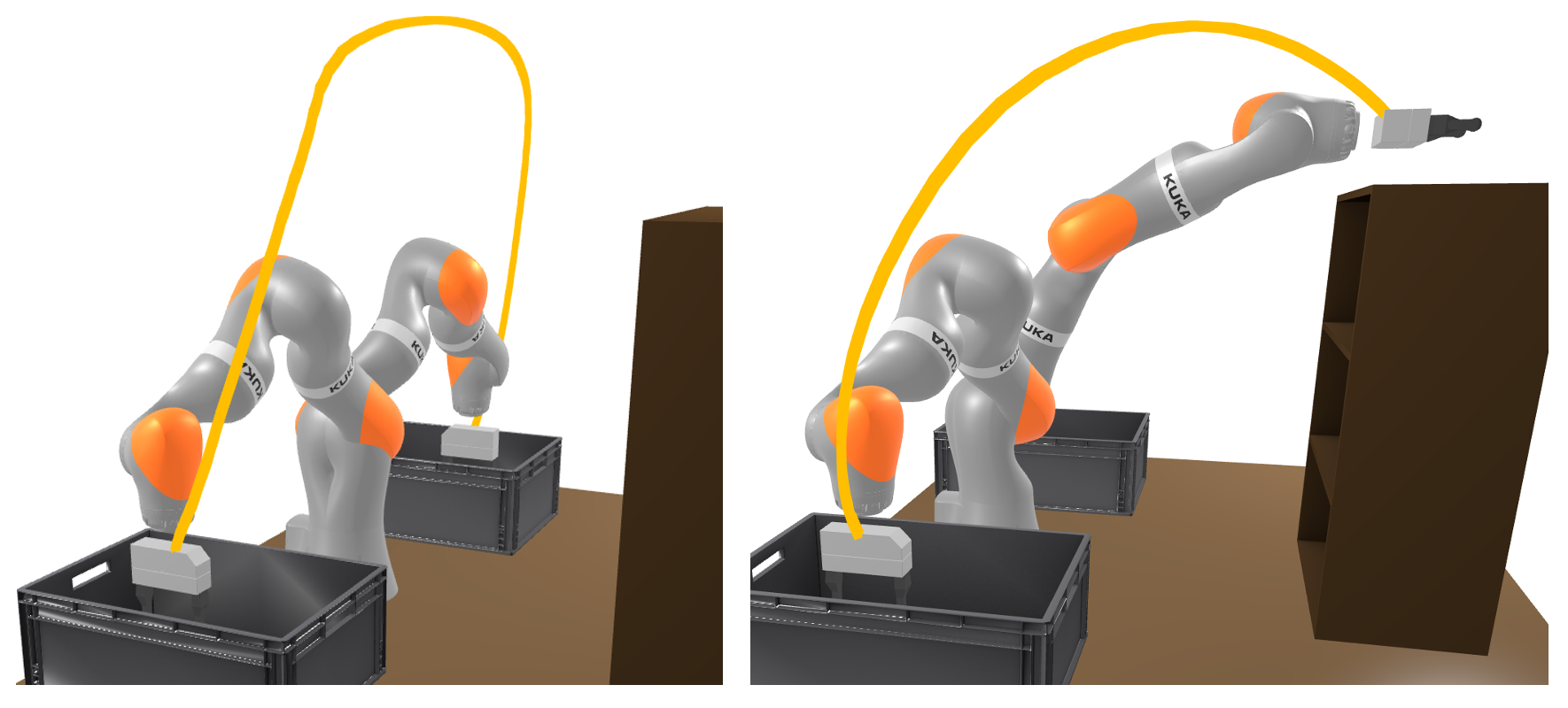
The experiments test a linearized contact pendulum and obstacle-aware planning for a seven-dimensional double integrator with robot-arm geometry. They study trajectory quality and relaxation tightness within these models.
VII-A Inverted Pendulum with Elastic Wall
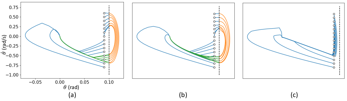
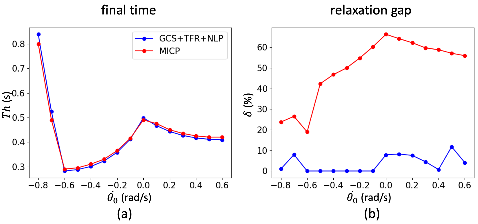
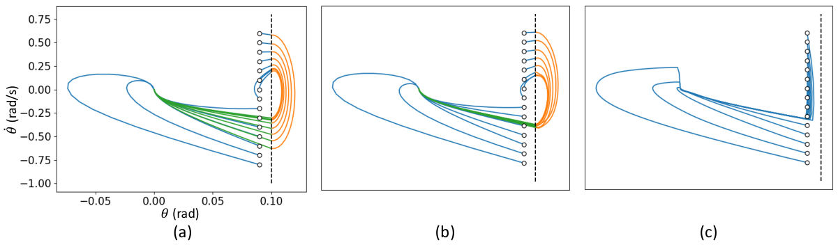
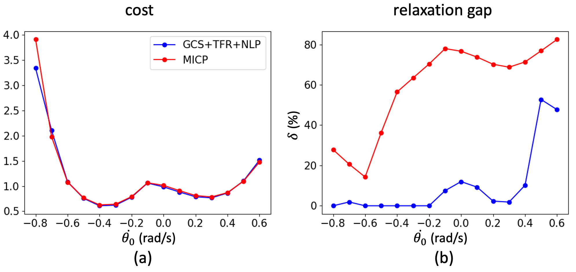
The contact-pendulum comparison uses 20 steps per mode with optimized durations, versus a fixed-step mixed-integer formulation with h=0.005 and 160 steps. The proposed relaxed trajectories closely follow nonlinear-refined solutions in the illustrated cases; the mixed-integer relaxation often misses wall contacts. Figures also evaluate a combined time-and-control-effort objective. Because the discretizations and timing freedom differ, their objectives should be interpreted within the corresponding formulations. The reported gap compares a relaxed lower bound with a feasible refined or mixed-integer solution, rather than directly measuring continuous-time physical optimality.
VII-B Robot Arm
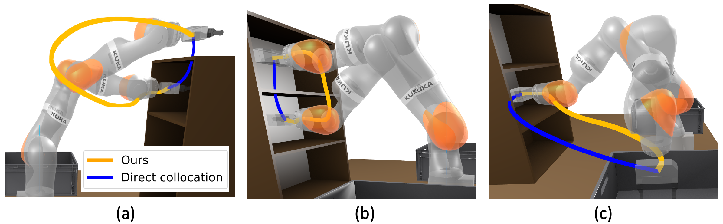
The arm experiment uses a seven-dimensional double-integrator approximation with LBR iiwa collision geometry, not full manipulator dynamics. IRIS-NP [49] approximately covers collision-free configuration space with ten convex regions. The planner selects a region sequence and a trajectory within that decomposition. Across five tasks, the tested direct-collocation setup fails to find collision-free paths, even with TFR initialization; this is a result for that implementation and problem setup.
Table I reports relaxation gaps of 0.9%, 2.1%, 14.3%, 24.4%, and 5.8%. Thus several solutions are close to their lower bounds, but the arm results do not establish uniformly near-zero gaps or exact global optimality. Full robot dynamics and coverage beyond the chosen convex-region decomposition remain outside the demonstrated model.
| Task | 0 | 1 | 2 | 3 | 4 |
|---|---|---|---|---|---|
| Relaxation gap (%) | 0.9 | 2.1 | 14.3 | 24.4 | 5.8 |
VIII Conclusion
The selective time-scaled lifting offers a useful compromise between weak first-order relaxations and expensive full higher-order relaxations. Its sparse and graph-based extensions support variable-duration hybrid planning, with nonlinear recovery and explicit gap estimates defining the practical guarantees. Empirical tightness should not be read as a theorem of exactness.
Appendix: complete relaxation. Equations 12–13 express dynamics, polytope constraints, and terminal conditions in lifted coordinates. They include the original constraints, products with trajectory and time variables, and scaled forms involving h and 1/h. Products of nonnegative linear inequalities add entrywise nonnegativity restrictions. Equation 14 matches shared-state moments across sparse blocks, including ordinary, time-weighted, and inverse-time-weighted products. All these original equations are retained below; they specify the tightening constraints essential to reproducing the relaxation.
Equations 12a–14
| (12a) | ||||
| subject to | (12b) | |||
| (12c) | ||||
| (12d) | ||||
| (12e) | ||||
| (13a) | ||||
| subject to | (13b) | |||
| (13c) | ||||
| (13d) | ||||
| (13e) | ||||
| (13f) | ||||
| (13g) | ||||
| (13h) | ||||
| (13i) | ||||
| (13j) | ||||
| (14) | ||||