Overview
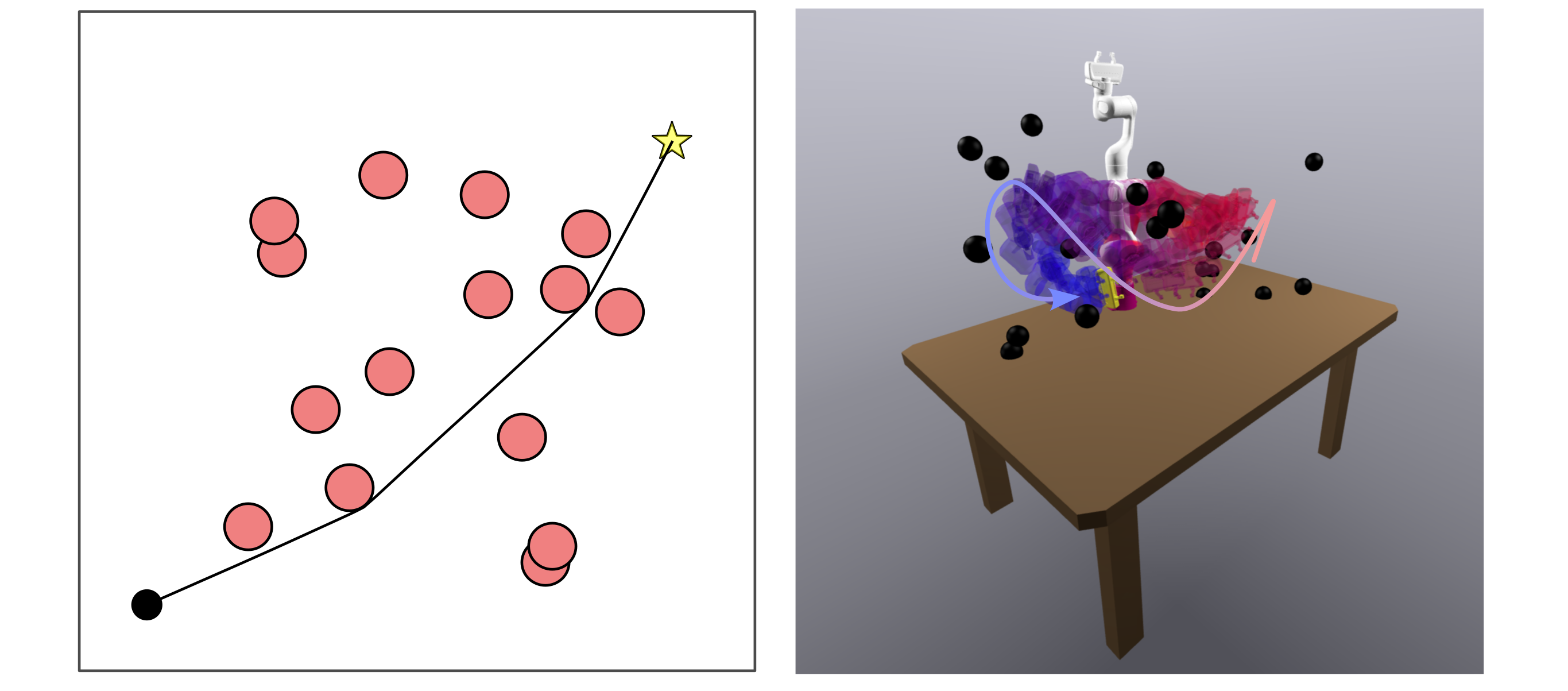
The complete setup figure retains the physical arm and depth cameras, the perceived obstacle model, and a two-dimensional slice through the seven-dimensional configuration space with the constructed regions.
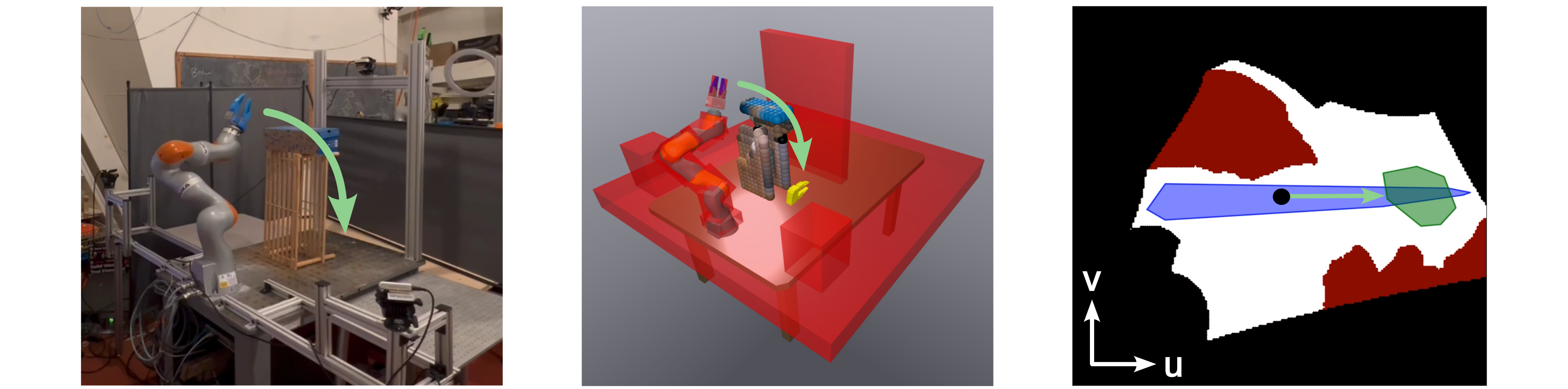
At a glance
EI-ZO inflates collision-free path segments into convex configuration-space regions using GPU-parallel sampling, collision checks and boundary searches. A dynamic roadmap first supplies a path; convex-set trajectory optimization then improves it, with collision checks and region repairs when needed. In two- and seven-dimensional simulation benchmarks, the sequence-based approaches improve conditional collision-free planning reliability and average speed relative to nonlinear trajectory optimization, at a trajectory-cost penalty. Fifteen hardware plans average 823 ms end to end. The regions are only probabilistically collision-free, the reported simulation results are conditioned on roadmap success, and obstacles are assumed stationary during each plan and execution.
I Introduction
Nonlinear trajectory optimization accommodates rich objectives and constraints but can fail from poor initialization. Sampling-based methods find routes but may produce inefficient motion. Decomposition-based motion planners move collision avoidance into a collection of convex free-space regions, leaving simpler trajectory constraints; constructing and positioning those regions has been the bottleneck in changing scenes.
This paper builds on IRIS-ZO [21] and inflates line segments rather than isolated points. Each region contains its seed segment, so regions along a valid polygonal path form a connected corridor. Constructing only this corridor avoids approximating the entire free space. Dynamic roadmaps supply the initial paths, GPU acceleration makes region construction fast, and a final repair loop handles residual collisions. The speed and reliability evidence concerns the tested pipeline, with precomputation and a working collision model.
II Assumptions
The robot model must provide kinematics and collision geometry, such as a URDF [23] or SDF [24]. Perceived obstacle geometry must support conservative checks: the collision checker is assumed never to label an actually colliding configuration safe. Added obstacles must remain stationary during the brief planning and execution interval. “Changing environments” therefore means updates between plans; the experiments do not validate avoidance of obstacles moving during execution.
III Background
The method combines probabilistic convex-region construction with path-guided placement.
III-A Constructing Safe Sets in Robot Configuration Space
IRIS variants iteratively separate sampled or optimized collision points from a candidate polytope. EI-ZO extends the zero-order variant because collision queries and simple updates parallelize well. Its guarantee bounds the probability that more than an ε fraction of the region’s volume is in collision by δ. This is a volume statement about the returned region, not a bound on collision probability of an arbitrary optimized trajectory. Exact polynomial certificates [19] solve a stronger problem at greater cost.
Equation 1
| (1) |
III-B Positioning Safe Sets for Effective Motion Planning
A global convex cover may need too many sets for online recomputation. A path corridor constructs only regions relevant to one route, as in earlier safe-flight corridors [12][13]. EI-ZO replaces an ellipsoidal distance metric with distance to a segment, allowing direct segment containment without ellipsoid optimization. This placement is efficient but inherits the route quality and connectivity available from the seed path.
IV Rapidly Inflating Line Segments
EI-ZO constructs full-dimensional polytopes around seed segments using only collision checks, projections and separating hyperplanes.

IV-A Preliminaries
Distance to a convex set is convex, so its sublevel sets are convex. At a colliding point outside a safe segment, the gradient of distance to that segment defines a supporting plane that separates the point while retaining the segment. Projection and gradient have closed-form expressions, including the degenerate case of coincident endpoints.
Starting from a large domain, the algorithm repeatedly removes collision points with such planes. Searching for collisions close to the segment tends to eliminate more distant collisions with fewer faces. A small step back from each collision permits finite approximations of concave obstacle boundaries; the practical step is reduced when necessary to avoid removing either seed endpoint. Infinite exact separation is replaced by a finite statistical stopping test.
Equations 2–8b
| (2) |
| (3) |
| (4a) | |||
| (4b) | |||
| (5) |
| (6) |
| (7) |
| (8a) | ||||
| (8b) | ||||
IV-B The EI-ZO Algorithm
The initial region is the domain, typically the joint-limit box. Each iteration draws a hit-and-run batch of size max(Np,M), where M is determined by ε, threshold τ and iteration confidence δk. The schedule δk = 6δ/(π²k²) allocates total uncertainty across iterations. If at most M(1−τ)ε of the first M samples collide, the unadaptive test accepts the region.
Otherwise, colliding samples are projected toward the segment and refined by a fixed number of bisection steps, retaining points on the colliding side. Candidates are sorted by distance to the segment; up to Nf separating planes are added, skipping candidates already removed by earlier planes. Sampling and refinement repeat until acceptance. The exact original pseudocode is retained; its sample call shows M, while the prose specifies max(Np,M). The guarantee presumes the required sampling/test assumptions and a correct collision checker.
Equations 9–10b
| (9) |
| (10a) | |||
| (10b) | |||
IV-C Practical Algorithmic Considerations
An optional iteration cap bounds construction time but explicitly voids the statistical guarantee if the test has not passed. Since the implementation checks seed paths by discretization, they can contain missed collisions. A candidate within collision tolerance of the segment triggers failure; checking its projection early can fail faster.
The step back is reduced whenever the maximum step would exclude a segment endpoint, preserving seed containment at the cost of potentially more faces. A rule of thumb selects the fixed bisection count as log₂(L/Δmax), where L estimates the largest boundary-search distance. Fewer steps can increase runtime by requiring more rounds of cuts; the method does not replace sampled path validation with a continuous collision certificate.
Equations 11–13
| (11) |
| (12) |
| (13) |
IV-D CUDA Implementation of EI-ZO
CSDecomp implements the method in C++/CUDA with Python bindings. GPU threads parallelize hit-and-run walks, forward kinematics, pairwise collision checks, projections and bisection. Candidate sorting and nonredundant-plane placement use one thread. Samples remain in GPU memory; only the seed segment and final polytope cross the CPU/GPU boundary. Current collision geometry supports boxes and spheres, and finite mixing steps approximate uniform sampling.
V Generating Collision-Free Polygonal Paths using Dynamic Roadmaps
Dynamic roadmaps [35] combine a precomputed probabilistic roadmap [36] with workspace-voxel lookup tables for quickly invalidating configurations after perception updates. Following GPU-accelerated roadmap work [38], this implementation stores node collisions and checks edges lazily online. Precomputation shifts substantial work out of online timing.
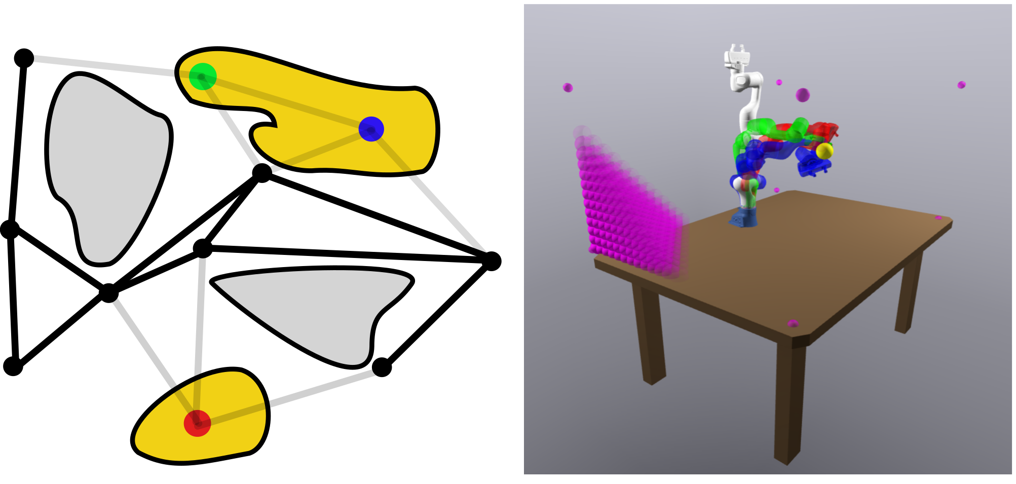
V-A Offline Roadmap Construction
Four maps store node configurations, adjacency, voxel-to-colliding-node associations and end-effector poses. Occupancy changes prune nodes using the lookup map. The offline construction is tied to the robot, geometry and workspace discretization; it is not rebuilt from scratch for every plan.
V-B Online Planning given Perception
Online planning activates voxels from the point cloud and collects their invalidated nodes. Nearby collision-free roadmap poses warm-start inverse kinematics for the goal. Start and goal configurations connect to the remaining graph; A* [41], lazy edge checks and greedy shortcutting produce a polygonal path. Circumscribed voxel spheres provide the obstacle geometry. Occlusions or modeling errors still matter because conservative perception is an assumption.
VI The Motion Planning Pipeline
The pipeline solves goal IK, searches the roadmap, inflates the path and optimizes inside the resulting regions. Candidate trajectories are discretely collision-checked; detected collisions trigger region cuts and reoptimization. It can also inflate multiple alternative routes for graph-based convex planners.
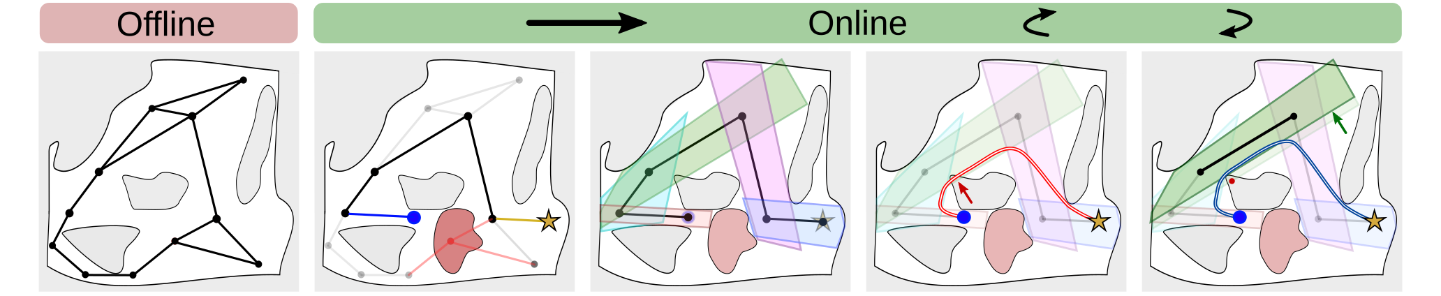
VI-A Inflating a Single Path
Segments are considered in order. A segment is inflated only if no existing region already contains it. Consecutive seed segments share endpoints, and containment therefore preserves a connected route from start to goal, provided the original path is truly collision-free.
VI-B Rapidly Recovering from Detected Collisions
Residual collision points on an optimized trajectory warm-start the same projection/bisection/cutting procedure. After modifying regions, the planner rechecks coverage of every original path segment: a cut preserves its own seed but can remove other segments previously covered incidentally. Uncovered segments receive new regions. Optimization and checking repeat until no sampled collisions remain. The loop’s empirical success does not furnish a continuous-time safety guarantee or a fixed worst-case runtime.
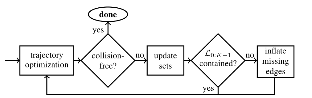
VI-C Inflating Multiple Paths
To obtain alternative routes, the heuristic selects an interior region containing neither endpoint, temporarily invalidates roadmap nodes inside it, reruns A*, and inflates the new path. It stops if this fails. Additional intersecting regions may reveal better paths to graph-based planners, but neither route diversity nor better optimized cost is guaranteed.
VII Experimental Evaluation
The evaluation uses synthetic planning problems and a perception-driven robot demonstration; it compares both path length and traversal-time objectives.
VII-A Simulation Benchmark
Simulation covers a two-dimensional obstacle field and a seven-joint arm. Four roadmap sizes, ten scene seeds and ten roadmap seeds produce 400 instances per optimization approach and problem setting.
VII-A 1 Environments
Forest places 15 radius-0.35 circles inside the central 7 × 7 area of a 10 × 10 square, with opposite-corner endpoints. Franka places 20 spheres in front of a seven-DOF FR3 arm; 33 robot spheres and a box table generate 1,187 collision pairs, including 527 self-collision pairs. Random starts lie on one side of the table and goal poses on the other.
VII-A 2 Problem Types
Minimum-distance planning minimizes polygonal path length. Minimum-time planning also enforces joint velocity/acceleration limits and zero velocity at both endpoints. The original objectives and constraints are preserved; these are kinematic planning problems rather than full dynamics or torque-constrained control.
Equations 14a–15f
| (14a) | ||||
| (14b) | ||||
| (14c) | ||||
| (15a) | ||||
| (15b) | ||||
| (15c) | ||||
| (15d) | ||||
| (15e) | ||||
| (15f) | ||||
VII-A 3 Baseline Approach
The nonlinear baseline uses Drake [42] and SNOPT or IPOPT, initialized from the same roadmap path. Collision constraints are imposed at finitely many points. Minimum-time initialization sets fourth-order B-spline control points from the roadmap path. Solver choices and collision-discretization counts are tuned separately by scene and task, so this is a particular implemented baseline rather than all nonlinear planning methods.
VII-A 4 Employed DBMPs
LSCS solves a shortest-path second-order cone program through one region sequence using MOSEK. LGCS inflates two routes and solves a mixed-integer graph-of-convex-sets formulation [46] with Gurobi. SCSTO uses SCSTrajopt [15] and Clarabel for minimum-time trajectories through a sequence, alternating convex subproblems. Global optimality of the graph problem remains restricted to its constructed regions.
VII-A 5 Results
On an i9-10850K and RTX 3090, Forest roadmaps contain 200–1,600 nodes and Franka roadmaps 3,000–12,000. Table I conditions optimization statistics on roadmap success: that prerequisite succeeds in all Forest cases and 96.1% of Franka cases. The single-sequence LSCS/SCSTO methods attain 100% conditional collision-free rate. The two-route LGCS Franka result is 99.3%, so the blanket “never failed” claim does not apply to every convex-set variant.
The reported headline averages are 17.1× speedup and a rise from about 72.1% to 100% conditional reliability: roughly 27.9 percentage points, not a 27.9% relative gain. Table I’s total optimization-stage time includes region construction and trajectory optimization, but not the preceding roadmap/IK/perception stages. For Franka, LSCS averages 152.5 ms versus NTO’s 3,084.6 ms; SCSTO averages 307.9 ms versus 4,147.8 ms. Full costs and empirical standard deviations remain in the table.
Among successful solutions, NTO finds lower-cost trajectories. Franka length is 5.519 versus 7.382 for LSCS (about 34% higher for LSCS relative to NTO), and traversal time is 5.057 versus 6.473 (about 28% higher). This is a material quality tradeoff, not uniformly a slight cost increase. Two-route LGCS offers only small length improvements while sharply increasing runtime. Region repair triggers in 5.6%/0.46% of Forest distance/time cases and 40.22%/21.36% of Franka cases.
| Problem | Minimum Distance | Minimum Time | ||||||||
| Environment | Forest | Franka | Forest | Franka | ||||||
| DRM SR | 1.00 | 0.961 | 1.00 | 0.961 | ||||||
| DRM num. LS | 3.450.86 | 4.491.24 | 3.450.86 | 4.491.24 | ||||||
| DRM path len. | 10.900.40 [m] | 8.552.28 [rad] | 10.900.40 [m] | 8.552.28 [rad] | ||||||
| TO Approach | NTO | LSCS | LGCS | NTO | LSCS | LGCS | NTO | SCSTO | NTO | SCSTO |
| cost (S only) | 10.7270.3 | 10.7700.3 | 10.7320.3 | 5.5191.1 | 7.3821.7 | 7.1101.6 | 9.3630.2 | 10.0960.7 | 5.0571.2 | 6.4731.5 |
| time total [ms] | 357.82520.3 | 18.29.8 | 96.8142.1 | 3084.62938.0 | 152.589.1 | 4441.610194 | 335.1167.2 | 19.37.8 | 4147.82674.6 | 307.9226.3 |
| time TO [ms] | 357.82520.3 | 13.95.7 | 91.3138.6 | 3084.62938.0 | 17.414.4 | 4236.510135 | 335.1167.2 | 15.96.1 | 4147.82674.6 | 189.1170.7 |
| time CS [ms] | - | 4.24.7 | 5.55.5 | - | 135.176.0 | 205.2107.8 | - | 3.42.6 | - | 118.861.0 |
| num. CS | - | 2.450.9 | 3.672.3 | - | 3.491.2 | 6.182.8 | - | 2.450.9 | - | 3.491.2 |
| TO SR | 0.993 | 1.000 | 1.000 | 0.863 | 1.000 | 0.993 | 0.459 | 1.000 | 0.735 | 1.000 |
| CFR | 0.970 | 1.000 | 1.000 | 0.725 | 1.000 | 0.993 | 0.459 | 1.000 | 0.732 | 1.000 |
| CFR given TO S | 0.977 | 1.000 | 1.000 | 0.840 | 1.000 | 1.000 | 1.000 | 1.000 | 0.995 | 1.000 |
VII-B Validation on Hardware
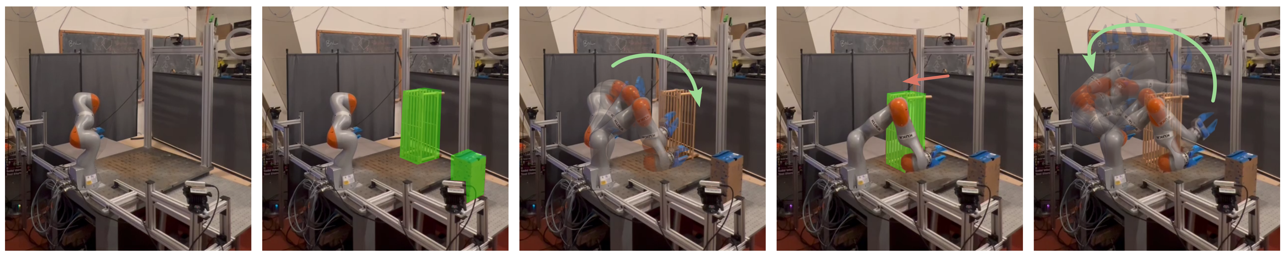
Hardware uses a KUKA LBR iiwa 7 R800, three RealSense D415 cameras, an i9-7900X and RTX 2080 Ti. Robot geometry has 11 boxes and 105 self-collision pairs. Joint velocity and acceleration bounds are ±1 rad/s and ±1 rad/s². The robot alternates between poses on opposite sides of a table, while obstacles are placed or moved between plans.
Fifteen trajectories have no observed planning failure. Total latency is 823.4 ± 122.6 ms: perception 369.7 ms, IK 130.1 ms, roadmap 116.8 ms, regions 122.5 ms and SCSTO 82.8 ms, plus overhead. Thus the 0.12-second region construction is only one part of online latency. The prose describes 8 cm perception voxels, while the offline roadmap parameter table gives 6 cm voxels; these different stages should not be silently conflated. This small demonstration does not establish a general failure rate or responsiveness to moving obstacles.
| Component | Time [ms] |
|---|---|
| perception | 369.7 16.7 |
| IK | 130.1 79.5 |
| DRM | 116.8 34.8 |
| convex sets | 122.5 43.1 |
| SCSTO | 82.8 67.9 |
| overhead | 1.5 0.6 |
| total | 823.4 122.6 |
| Auxiliary Stats. | Value |
|---|---|
| num. line seg. | 2.9 0.6 |
| num. safe sets | 1.93 0.57 |
| col. checks / set | 121018 24262 |
| hyperplanes / set | 60.7 14.4 |
| voxels | 359.6 76.4 |
| col. pairs | 4431.2 916.7 |
| self-col. pairs | 105 |
VIII Limitations
The principal limits are region-constrained solution quality, memory-intensive geometry checking, untested higher-dimensional scaling and weak goal IK.
VIII-A Local and Global Improvements with Nonlinear Solvers
Convex planners cannot leave the constructed region union, so poor seed paths or overly small regions can exclude good trajectories. A nonlinear optimizer can sometimes escape its initialization and reach a lower-cost solution, explaining part of the observed tradeoff. Multiple inflated paths only modestly help in these tests. Conversely, failed plans can carry operational costs absent from successful-only trajectory averages.
VIII-B GPU Memory
The collision checker evaluates configurations against voxel obstacles in parallel; finer three-dimensional grids increase memory use cubically with resolution. Signed-distance-field representations [49][50] are proposed future work, not part of the evaluated implementation.
VIII-C Scaling to Higher Dimensions
Only two- and seven-dimensional systems are tested. Mobile manipulation, bimanual systems and larger configuration spaces may challenge both roadmap coverage and region sampling; their scalability remains unverified.
VIII-D Inverse Kinematics
Hardware goal poses are deliberately not overlapped by obstacles, producing relatively simple IK problems. The authors identify IK as a weak point but do not stress-test it. Robot-specific analytic IK [52] is a possible improvement.
IX Conclusion
EI-ZO makes path-guided convex-region generation fast enough for repeated planning in scenes that change between motions. In these benchmarks, single-sequence planning trades higher trajectory cost for better conditional reliability and lower optimization latency. Its useful complementarity with faster sampling planners and richer convex-set optimizers does not remove assumptions about perception, static execution scenes, valid seed paths or sampled collision checks.
Acknowledgments
The authors acknowledge discussions, SCSTrajopt code, software/hardware assistance and funding from Toyota Research Institute.
Appendix A Appendix
The appendix retains the convexity proof, roadmap construction, complete shortest-path formulation and all implementation parameters.
A-A Distance Function Convexity
The proof combines triangle inequality with convexity of the target set: a convex combination of nearest points remains in the set, so distance at a convex combination of query points is no greater than the corresponding weighted distances. The original three displayed steps are retained. As written, the argument assumes the distance minimizers exist, which holds for the closed line-segment seed used here.
Equations 16–18
| (16) | ||||
| (17) | ||||
| (18) | ||||
A-B DRM Construction
Offline construction samples collision-free configurations, connects nearby nodes subject to configuration-space and task-space distance thresholds, limits neighbors, and symmetrizes adjacency. Each workspace voxel is represented by its circumscribing sphere of radius √3 s/2. Checking every voxel against roadmap nodes builds the collision lookup map; online edge checks remain lazy.
A-C Polygonal Shortest Paths through Sequences of Convex Sets
The intended LSCS objective minimizes total Euclidean distance between adjacent knot points, with start/goal endpoints and successive-region intersection constraints. Equation 19 is preserved exactly but contains an apparent transcription error: (19d) imposes vi = vi+1 for every segment, forcing all knots equal and making distinct endpoints infeasible. The variable range also starts at v0 while the endpoint constraint uses v1. These printed equations should be reconciled with the implementation before treating them as runnable optimization specifications.
Equations 19a–19f
| (19a) | ||||
| (19b) | ||||
| (19c) | ||||
| (19d) | ||||
| (19e) | ||||
| (19f) |
A-D Supplementary Information on Experimental Evaluation
Simulation uses Ubuntu 22.04, CUDA 12.6 and an RTX 3090. At batches of two million configurations, collision-check throughput is about 19.9 million/s for Forest and 8.6 million/s for Franka. SNOPT is used for both Forest tasks with 20/100 collision points; Franka uses SNOPT for distance and IPOPT for time, with 150 points. Lazy path checks use steps of 0.1 m or 0.1 rad. These batch throughputs do not imply equivalent end-to-end planning rates.
Forest EI-ZO uses δ = 0.05, ε = 0.01, 1,000 update samples, ten faces per iteration, 30 mixing steps and step back 0.01. Franka uses δ = ε = 0.005, 10,000 samples, ten faces, 60 mixing steps and the same step back. Acceptance typically occurs within ten iterations; this observation is not an iteration guarantee. Tables III–VI retain every parameter.
Hardware uses CUDA 12.5, a 35,000-node roadmap and the Franka EI-ZO settings with 20 faces per iteration. Collision checking reaches about 6.9 million configurations/s at a two-million batch. No region repair was triggered in the 15 hardware examples. The offline roadmap uses a 0.45 m task-space neighbor limit, 4.5 rad configuration-space limit, ten neighbors and 0.06 m voxel side length.
| Parameter | Symbol | Value |
|---|---|---|
| admissible uncertainty | 0.05 | |
| admissible fraction in collisions | 0.01 | |
| number of samples to update | 1000 | |
| max number of faces per iteration | 10 | |
| number of mixing steps for sampling | 30 | |
| step back | 0.01 |
| Parameter | Symbol | Value |
|---|---|---|
| admissible uncertainty | 0.005 | |
| admissible fraction in collision | 0.005 | |
| number of samples to update | 10000 | |
| max number of faces per iteration | 10 | |
| number of mixing steps for sampling | 60 | |
| step back | 0.01 |
| Parameter | Symbol | Value |
|---|---|---|
| max. task space distance | 10 [m] | |
| max. configuration space distance | 10 [m] | |
| max. neighbors | 10 | |
| offline voxel length | 0.06 [m] |
| Parameter | Symbol | Value |
|---|---|---|
| max. task space distance | 0.45 [m] | |
| max. configuration space distance | 4.5 [rad] | |
| max. neighbors | 10 | |
| offline voxel length | 0.06 [m] |