Overview
This edition includes the complete v2 supplement, metric definitions, model configurations, and prompt templates. Rankings describe the tested versions and benchmark settings; scores are normalized evaluation proxies rather than probabilities of successful world generation.
| Benchmark | # Examples | Multi-Scene | Unified | Long Seq. | Image Cond. | Multi-Style | Camera Ctrl. | 3D Consist. |
| TC-Bench [15] | 150 | ✗ | ✗ | ✗ | ✓ | ✗ | ✗ | ✗ |
| EvalCrafter [45] | 700 | ✗ | ✗ | ✗ | ✗ | ✗ | ✗ | ✗ |
| FETV [46] | 619 | ✗ | ✗ | ✗ | ✗ | ✗ | ✗ | ✗ |
| VBench [26] | 800 | ✗ | ✗ | ✗ | ✗ | ✗ | ✗ | ✗ |
| T2V-CompBench [71] | 700 | ✗ | ✗ | ✗ | ✗ | ✗ | ✗ | ✗ |
| Meng et al. [48] | 160 | ✗ | ✗ | ✗ | ✗ | ✗ | ✗ | ✗ |
| Wang et al. [78] | 423 | ✗ | ✗ | ✓ | ✗ | ✗ | ✗ | ✗ |
| ChronoMagic-Bench [92] | 1649 | ✗ | ✗ | ✗ | ✗ | ✗ | ✗ | ✗ |
| WorldModelBench [40] | 350 | ✗ | ✗ | ✗ | ✓ | ✗ | ✗ | ✗ |
| WorldScore (Ours) | 3000 | ✓ | ✓ | ✓ | ✓ | ✓ | ✓ | ✓ |
At a glance
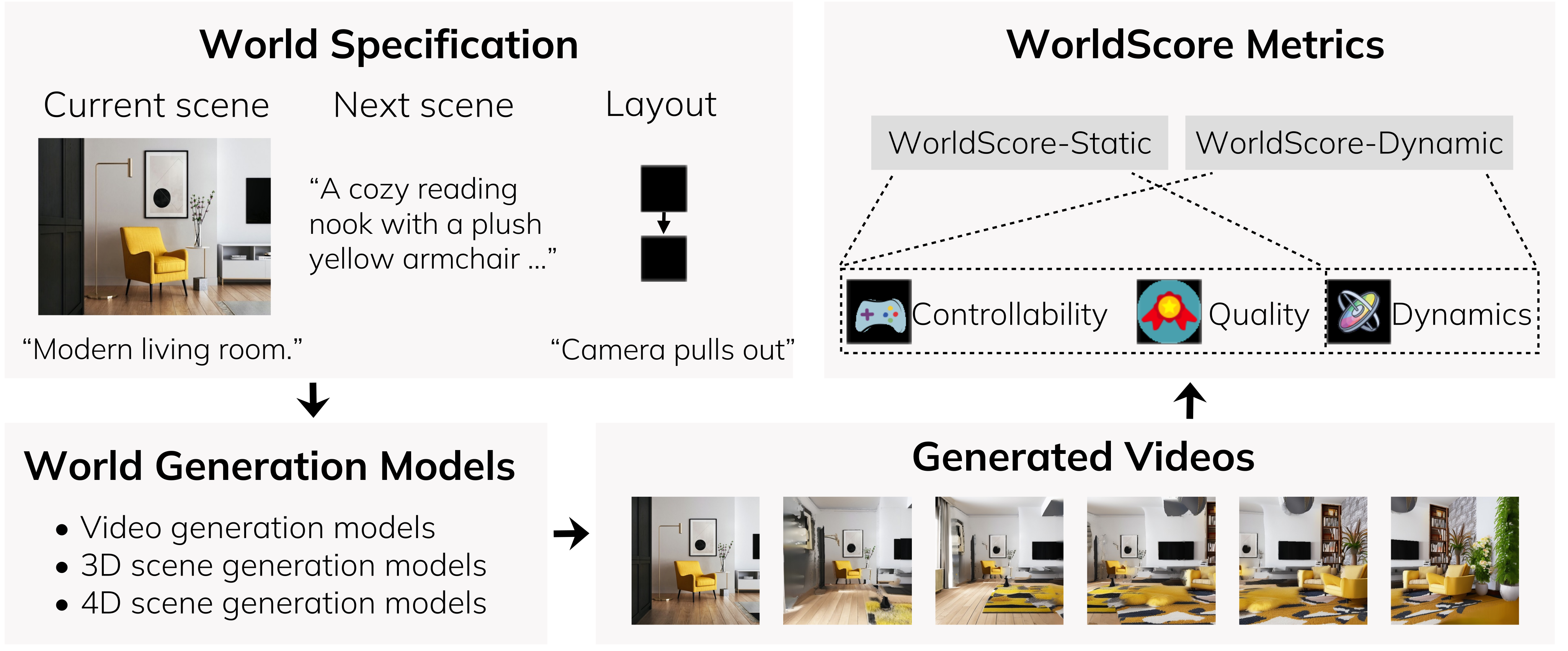
WorldScore evaluates world generation as a sequence of instructed scene transitions. Each task provides a current-scene image and text, a next-scene description, and a camera trajectory in both matrix and text form. Different 3D, 4D, image-to-video, and text-to-video generators produce videos that can be scored through a common interface.
The benchmark contains 3,000 static/dynamic and photorealistic/stylized examples. Ten metrics cover controllability, quality, and dynamics. Evaluation of 20 selected model configurations finds strong static-world performance for explicit 3D methods and weaker camera control in video generators. The dataset, evaluation code, leaderboard, and explanatory videos accompany the paper.
1 Introduction
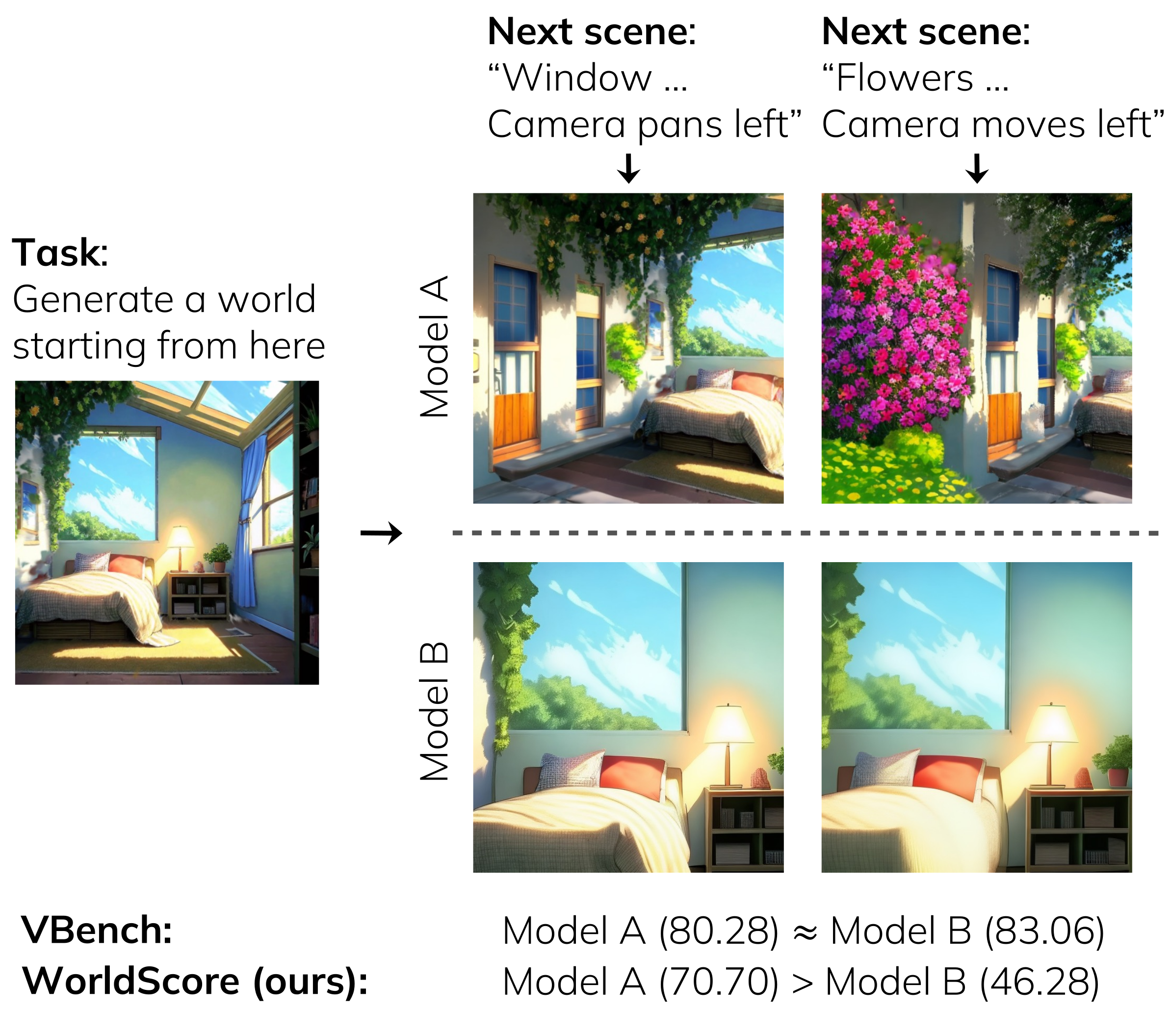
Producing an attractive single scene does not establish that a generator can move through a coherent world while following spatial instructions. WorldScore therefore tests transitions between specified scenes and separates static-world construction from in-scene dynamic motion.
Unlike a text-only video benchmark, it supplies images and explicit camera paths as well as text. This accommodates models with different interfaces, although their conditioning strength remains different: camera-matrix control is more precise than a verbal request.
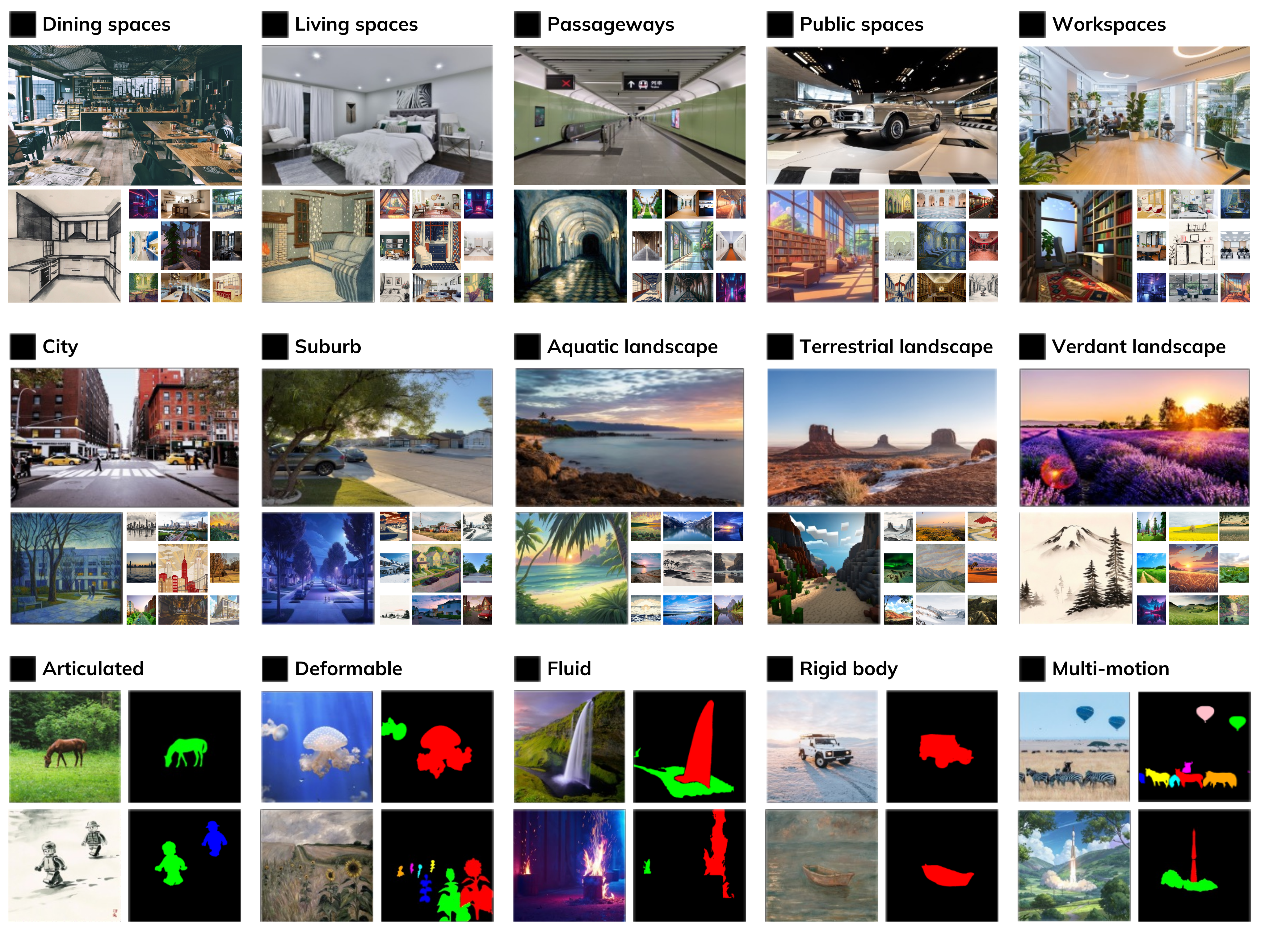
The dataset spans indoor/outdoor scenes, visual styles, short/long transitions, and five motion types. Common rendered videos make outputs comparable, but the resulting measurements still depend on the chosen estimators, prompt distribution, normalization, and task-specific model adapters.
2 Related Work
Benchmarks such as VBench emphasize video-generation quality, while WorldScore adds explicit layout control and multi-scene tasks compatible with 3D/4D methods. Table 1 retains the paper’s comparison of benchmark features; it reflects the cited versions rather than an exhaustive current survey.
Video generators can produce dynamic appearances without an explicit geometric scene. Many 3D scene generators instead extend views using image outpainting and estimated depth, obtaining direct camera control and consistent geometry. Scene-level 4D generation remains difficult; 4D-fy is included because an open implementation was available.
3 The WorldScore Benchmark
The benchmark standardizes three components: a world specification, a curated set of examples, and metrics computed from generated or rendered videos. Model-specific preprocessing translates the specification into the controls each model supports.
3.1 World Specification
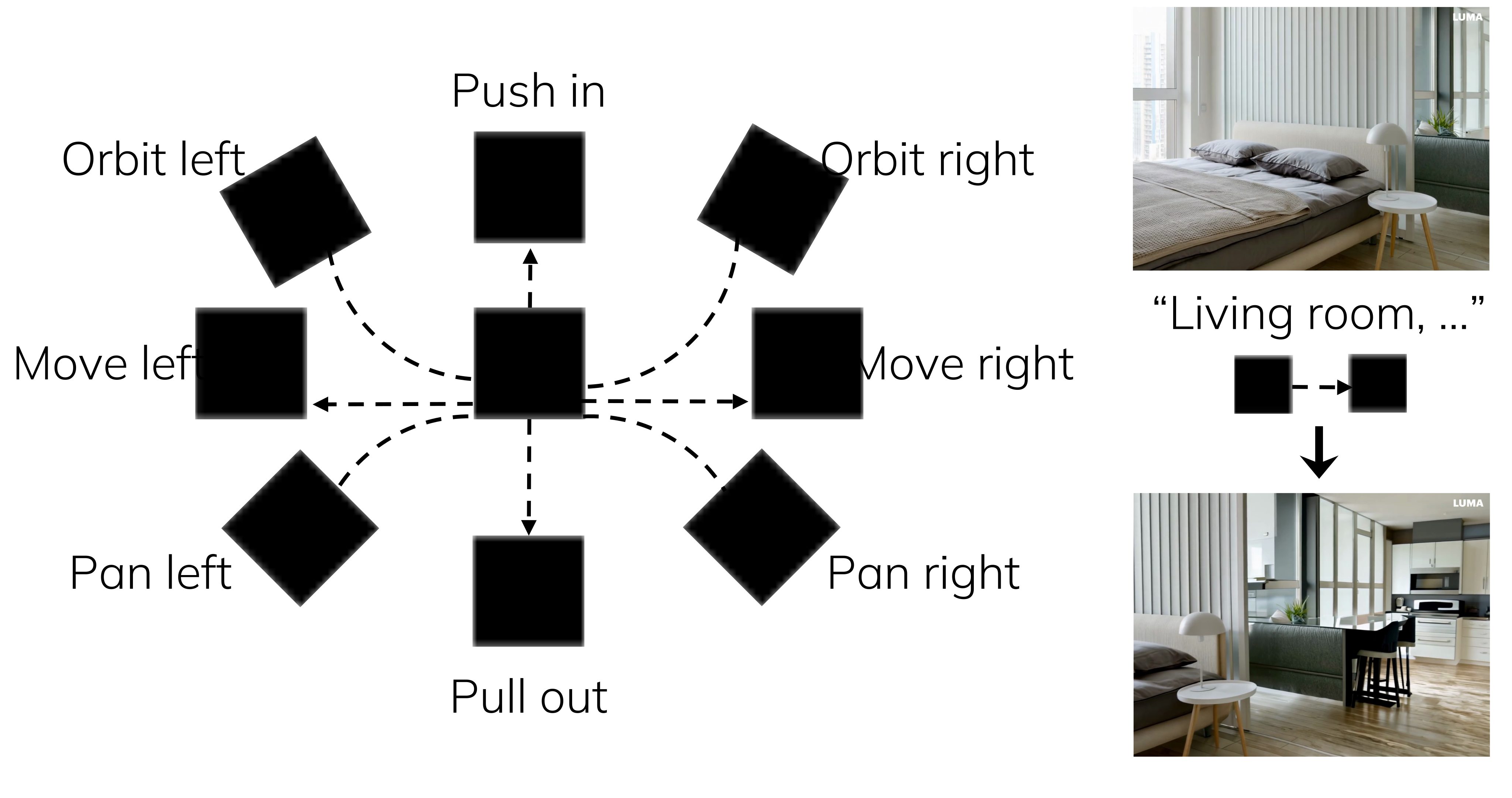
A step is a triplet of current scene, next scene, and layout. The current scene includes an image and caption; the next scene is described in text; layout includes a sequence of camera matrices and a verbal camera-motion instruction. Equation 1 expresses generation after a model-specific preprocessing function.
Static tasks request scene transitions under substantial camera movement and measure control/quality. Dynamic tasks keep the intended camera fixed and request motion within the current scene. Thus the benchmark does not directly test simultaneous large camera navigation and dynamic multi-scene interaction in one task.
Equation 1
| (1) |
3.2 Dataset Curation
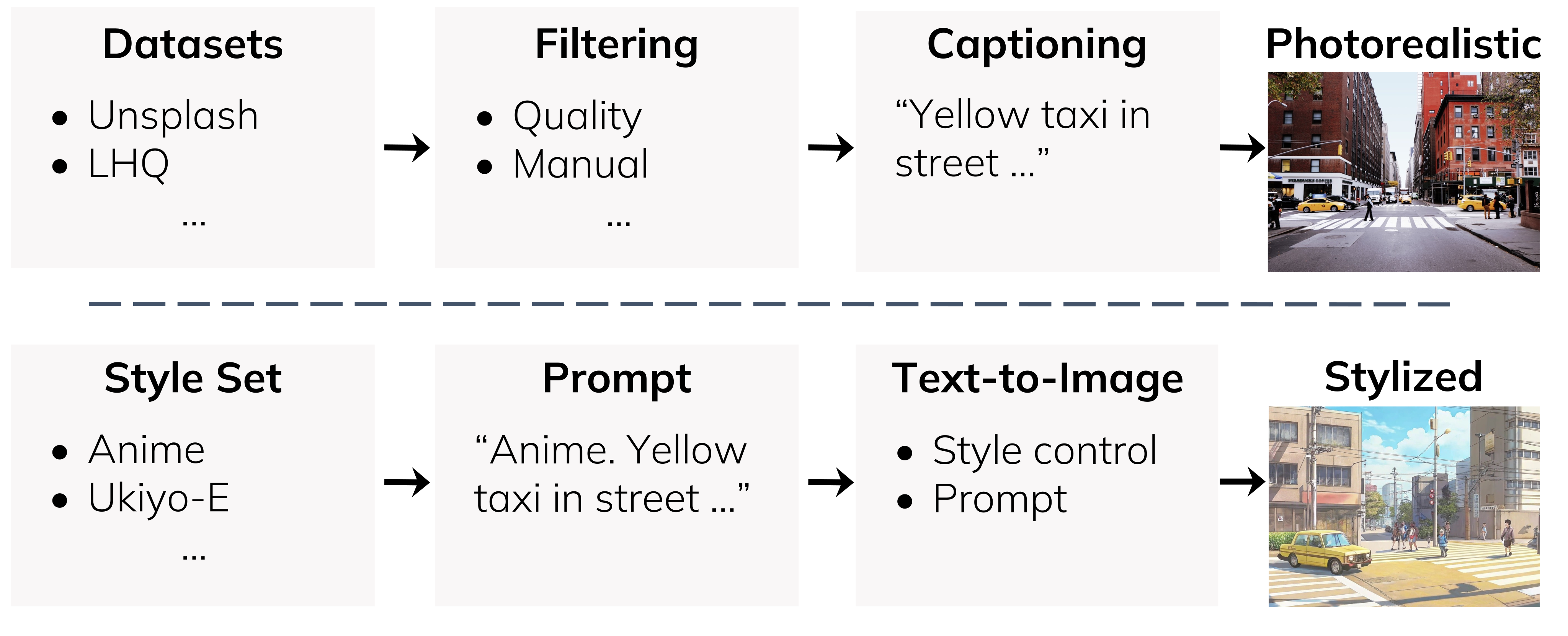
The static subset has 2,000 examples: five indoor and five outdoor categories, each with 100 photorealistic images and 100 stylized counterparts. Filtering reduces source datasets and Unsplash images to about 5,000 candidates before GPT-4o captioning/classification and quality selection. The final photorealistic set has 1,000 images; Recraft generates corresponding stylized scenes.
The dynamic subset has 1,000 examples: 100 photorealistic and 100 stylized images for each of articulated, deformable, fluid, rigid-body, and mixed motion. It includes first-frame masks identifying intended moving regions.
GPT-4o generates contextually linked next-scene descriptions. Eighty percent of static examples request one new scene; 20% request three, yielding four-scene worlds including the starting scene. Generated prompts are specifications, not observed ground-truth future worlds.
Eight camera movements cover push in, pull out, lateral movement, panning, and orbiting left/right. A randomly assigned movement accompanies each static transition. For an intra-scene movement, the next-scene prompt is replaced with the current-scene description so that the model should explore the same scene.
Equation 2
| (2) |
3.3 The WorldScore Metrics
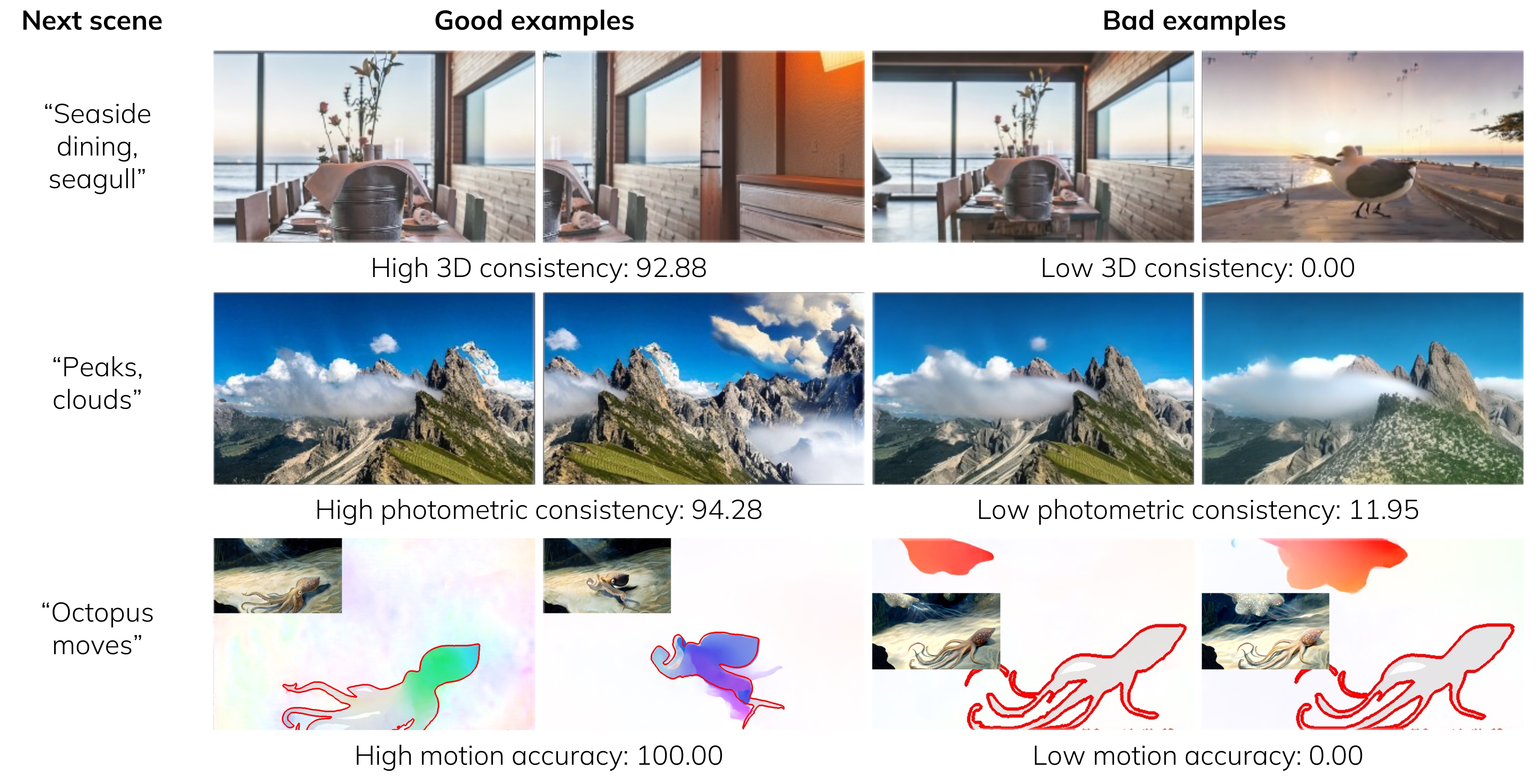
Controllability comprises camera-path error, detection of one or two prompted objects using Grounding DINO, and full-prompt CLIPScore alignment. Camera error is the geometric mean of rotation and scale-aligned translation errors. Object detection checks presence, not all relationships or physical properties requested by the prompt.
Quality comprises estimated 3D reprojection consistency, forward/backward optical-flow consistency, first-to-last-frame style Gram-matrix distance, and a learned perceptual-quality ensemble. These are distinct proxies but are not statistically independent or perfect separations of geometry and appearance.
Dynamics comprises motion inside the intended mask relative to outside, median flow magnitude, and agreement with interpolated missing frames. Large or smooth motion alone need not follow the requested action; background movement and estimator failures can affect these scores.
WorldScore-Static averages seven normalized control/quality dimensions. WorldScore-Dynamic averages all ten dimensions, including those seven static scores. Unsupported dynamics in 3D methods receive zero, making their dynamic aggregate 0.7 times the static aggregate. Scores are scaled to 0–100 after clipping and empirical calibration; they are not percentages of correct tasks.
Equation 3
| (3) |
| Models | WorldScore | Controllability | Quality | Dynamics | ||||||||
|
-Static
|
-Dynamic
|
Camera
Ctrl
|
Object
Ctrl
|
Content
Align
|
Consist
|
Photo
Consist
|
Style
Consist
|
Subjective
Qual
|
Motion
Acc
|
Motion
Mag
|
Motion
Smooth
| |
| Gen-3 [58] | 60.71 | 57.58 | 29.47 | 62.92 | 50.49 | 68.31 | 87.09 | 62.82 | 63.85 | 54.53 | 27.48 | 68.87 |
| Hailuo [20] | 57.55 | 56.36 | 22.39 | 69.56 | 73.53 | 67.18 | 62.82 | 54.91 | 52.44 | 63.46 | 27.20 | 70.07 |
| DynamiCrafter [84] | 52.09 | 47.19 | 25.15 | 47.36 | 25.00 | 72.90 | 60.95 | 78.85 | 54.40 | 41.11 | 39.25 | 26.92 |
| VideoCrafter1-T2V [9] | 47.10 | 43.54 | 21.61 | 50.44 | 60.78 | 64.86 | 51.36 | 38.05 | 42.63 | 11.76 | 75.00 | 18.87 |
| VideoCrafter1-I2V [9] | 50.47 | 47.64 | 25.46 | 24.25 | 35.27 | 74.42 | 73.89 | 65.17 | 54.85 | 55.63 | 25.00 | 42.49 |
| VideoCrafter2 [9] | 52.57 | 47.49 | 28.92 | 39.07 | 72.46 | 65.14 | 61.85 | 43.79 | 56.74 | 47.12 | 30.40 | 29.39 |
| T2V-Turbo [41] | 45.65 | 40.20 | 27.80 | 30.68 | 69.14 | 38.72 | 34.84 | 49.65 | 68.74 | 34.87 | 40.09 | 7.48 |
| EasyAnimate [86] | 52.85 | 51.65 | 26.72 | 54.50 | 50.76 | 67.29 | 47.35 | 73.05 | 50.31 | 75.00 | 31.16 | 40.32 |
| Allegro [97] | 55.31 | 51.97 | 24.84 | 57.47 | 51.48 | 70.50 | 69.89 | 65.60 | 47.41 | 54.39 | 40.28 | 37.81 |
| Vchitect-2.0 [14] | 42.28 | 38.47 | 26.55 | 49.54 | 65.75 | 41.53 | 42.30 | 25.69 | 44.58 | 33.59 | 33.81 | 21.31 |
| LTX-Video [19] | 55.44 | 56.54 | 25.06 | 53.41 | 39.73 | 78.41 | 88.92 | 53.50 | 49.08 | 76.22 | 29.95 | 71.09 |
| CogVideoX-T2V [88] | 54.18 | 48.79 | 40.22 | 51.05 | 68.12 | 68.81 | 64.20 | 42.19 | 44.67 | 25.00 | 47.31 | 36.28 |
| CogVideoX-I2V [88] | 62.15 | 59.12 | 38.27 | 40.07 | 36.73 | 86.21 | 88.12 | 83.22 | 62.44 | 69.56 | 26.42 | 60.15 |
| SceneScape [16] | 50.73 | 35.51 | 84.99 | 47.44 | 28.64 | 76.54 | 62.88 | 21.85 | 32.75 | 0.00 | 0.00 | 0.00 |
| Text2Room [24] | 62.10 | 43.47 | 94.01 | 38.93 | 50.79 | 88.71 | 88.36 | 37.23 | 36.69 | 0.00 | 0.00 | 0.00 |
| LucidDreamer [11] | 70.40 | 49.28 | 88.93 | 41.18 | 75.00 | 90.37 | 90.20 | 48.10 | 58.99 | 0.00 | 0.00 | 0.00 |
| WonderJourney [90] | 63.75 | 44.63 | 84.60 | 37.10 | 35.54 | 80.60 | 79.03 | 62.82 | 66.56 | 0.00 | 0.00 | 0.00 |
| InvisibleStitch [12] | 61.12 | 42.78 | 93.20 | 36.51 | 29.53 | 88.51 | 89.19 | 32.37 | 58.50 | 0.00 | 0.00 | 0.00 |
| WonderWorld [91] | 72.69 | 50.88 | 92.98 | 51.76 | 71.25 | 86.87 | 85.56 | 70.57 | 49.81 | 0.00 | 0.00 | 0.00 |
| 4D-fy [3] | 27.98 | 32.10 | 69.92 | 55.09 | 0.85 | 35.47 | 1.59 | 32.04 | 0.89 | 22.22 | 22.88 | 80.06 |
4 Results
The study evaluates 20 configurations: 13 video generators, six 3D scene generators, and one 4D generator. The source gives inconsistent I2V/T2V totals in the introduction and results prose; Table S1 lists eight I2V and five T2V video configurations, including both VideoCrafter1 and CogVideoX variants.
Model versions, output dimensions, durations, frame rates, and measured generation times remain in Table S1. These settings are not compute-matched. In particular, 4D-fy’s iterations are reduced to shorten an approximately 20-hour generation to the reported three hours, so its result is not a full-budget evaluation.
Human-preference studies and a resolution-change test assess the metrics. Their evidence supports selected comparisons under this protocol; neither establishes that the aggregate ranks all world-generation capabilities or all later model releases.
4.1 Observations and Challenges
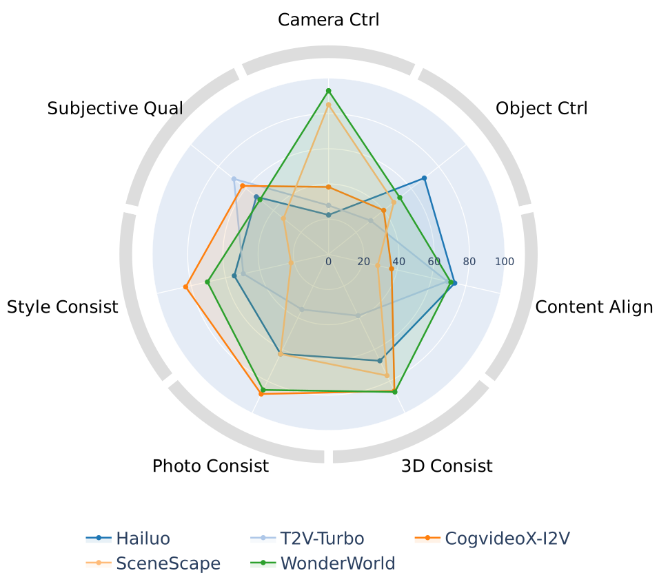
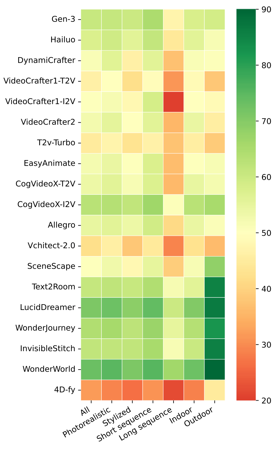
WonderWorld and LucidDreamer lead WorldScore-Static at 72.69 and 70.40. CogVideoX-I2V is the highest video model at 62.15. Explicit 3D methods receive camera matrices and score highly on camera and geometric consistency; video models receive text motion requests and all have much lower camera control.
CogVideoX-I2V also leads the tested video models on WorldScore-Dynamic at 59.12, ahead of Gen-3 and Hailuo, but loses to them on some object/content dimensions. This is a comparison of listed versions under the benchmark’s weighting, not general equivalence between open and closed systems.
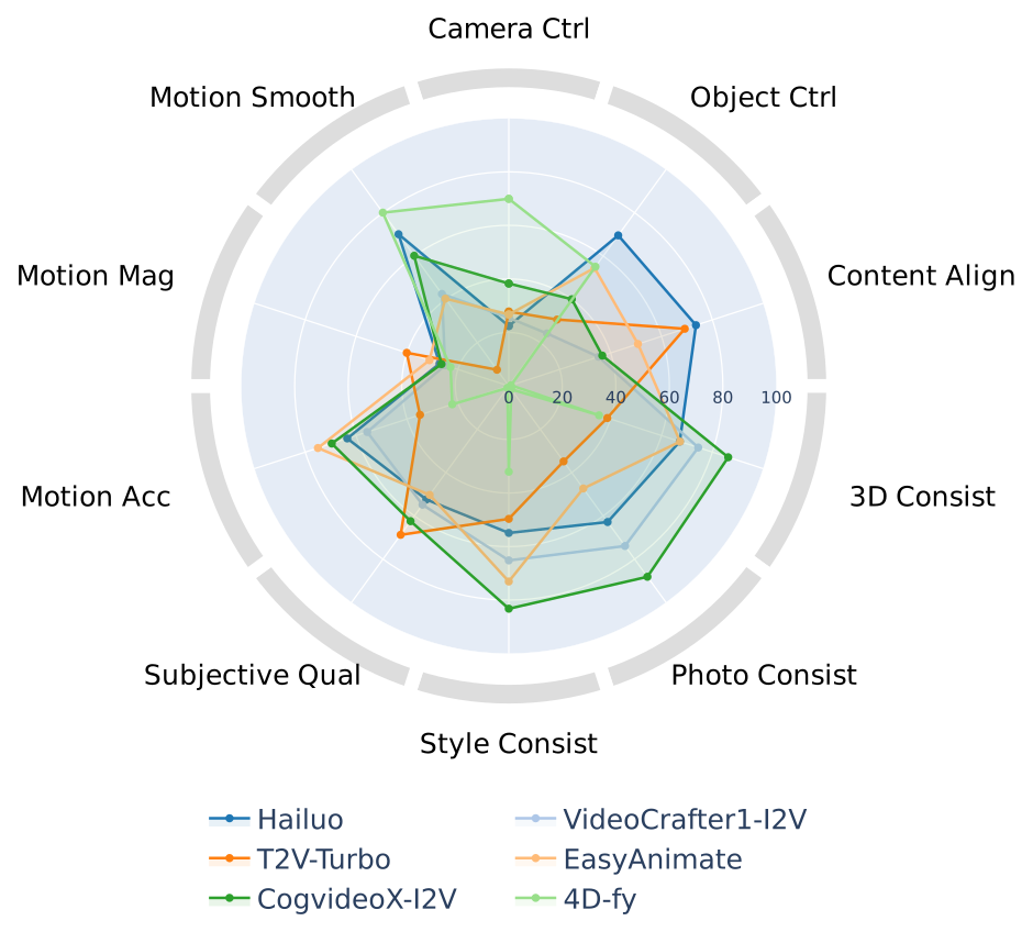
Large motion often accompanies lower smoothness, and motion magnitude does not reliably imply correct placement. Video methods also struggle on longer scene chains and outdoor scenes in the subdomain plot. Figure 7 plots 19 models and omits LTX-Video despite its inclusion in the main table. The T2V/I2V comparisons suggest greater camera movement and control for some T2V variants, versus higher visual quality for I2V variants; they do not isolate conditioning modality from every architecture/training difference.
4D-fy scores poorly overall in its reduced-budget configuration, while the static 3D methods receive zero dynamics scores by definition. This supports the difficulty of combining controllable geometry with motion, without establishing a limit of all 4D representations.
5 Conclusion
WorldScore turns broad world-generation claims into explicit scene, layout, appearance, and motion tests. The observed weaknesses motivate better camera control, longer coherent sequences, and methods combining geometric consistency with dynamics.
Interpret rankings with the metric estimators, unequal control interfaces, calibration bounds, and tested compute settings in view. The work acknowledges ONR, NSF, the Okawa Foundation, and discussions with Mohamed El Banani and Christoph Lassner.
Appendix A Additional Details on World Specification
Input images are center-cropped and resized to each model’s required resolution. I2V models use the reference image; T2V models receive the text specification and ignore image conditioning. Models supporting explicit cameras receive transformed poses in their own conventions; others receive camera-motion text appended to the next-scene prompt.
This permits common tasks across different interfaces, but does not give every model identical information or equally precise spatial control. Table S1 retains all generation settings and the reduced-iteration caveat for 4D-fy.
| Method | Version | Ability | Resolution | Length (s) | FPS | Open Source | Speed† | Camera§ |
| Gen-3 [58] | 24.07.01 | I2V | 1280×768 | 10 | 24 | ✗ | 1 min | ✗ |
| Hailuo [20] | 24.08.31 | I2V | 1072×720 | 5.6 | 25 | ✗ | 3.5 min | ✗ |
| DynamiCrafter [84] | 23.10.18 | I2V | 1024×576 | 5 | 10 | ✓ | 2.5 min | ✗ |
| VideoCrafter1 [9] | 23.10.30 | T2V | 1024×576 | 2 | 8 | ✓ | 7 min | ✗ |
| I2V | 512×320 | 2 | 8 | ✓ | 2 min | ✗ | ||
| VideoCrafter2 [10] | 24.01.17 | T2V | 512×320 | 2 | 8 | ✓ | 2 min | ✗ |
| T2V-Turbo [41] | 24.05.29 | T2V | 512×320 | 3 | 16 | ✓ | 5 s | ✗ |
| EasyAnimate [86] | 24.05.29 | I2V | 1344×768 | 6 | 8 | ✓ | 16 min | ✗ |
| CogVideoX [88] | 24.08.12 | T2V | 720×480 | 6 | 8 | ✓ | 2.4 min | ✗ |
| I2V | 720×480 | 6 | 8 | ✓ | 2.4 min | ✗ | ||
| Allegro [97] | 24.10.20 | I2V | 1280×720 | 6 | 15 | ✓ | 0.5 h | ✗ |
| Vchitect-2.0 [97] | 25.01.14 | T2V | 768×432 | 5 | 8 | ✓ | 2.8 min | ✗ |
| LTX-Video [19] | 25.05.05 | I2V | 768×512 | 4 | 30 | ✓ | 2.4 min | ✗ |
| SceneScape [16] | 23.02.02 | T2V | 512×512 | 5 | 10 | ✓ | 11.4 min | ✓ |
| Text2room [24] | 23.03.21 | I2V | 512×512 | 5 | 10 | ✓ | 12.4 min | ✓ |
| LucidDreamer [11] | 23.11.22 | I2V | 512×512 | 5 | 10 | ✓ | 6.4 min | ✓ |
| WonderJourney [90] | 23.12.06 | I2V | 512×512 | 5 | 10 | ✓ | 6.3 min | ✓ |
| InvisibleStitch [12] | 24.04.30 | I2V | 512×512 | 5 | 10 | ✓ | 2.3 min | ✓ |
| WonderWorld [91] | 24.06.13 | I2V | 512×512 | 5 | 10 | ✓ | 10 s | ✓ |
| 4D-fy [3]∗ | 23.11.29 | T2V | 256×256 | 4 | 30 | ✓ | 3 h | ✓ |
Appendix B Additional Details on Dataset Curation
The curation supplement records source datasets, automatic/manual filtering, seven visual styles, the exact GPT-4o prompts, generated examples, and category counts.
|
Scene
Type
|
Dataset
|
Image
Type
|
Res.
|
# Images
|
| Indoor | InterviorVerse [98] | Synthetic | 640×480 | 50,000 |
| Hypersim [57] | Synthetic | 1024×768 | 77,400 | |
| SUN-RGBD [69] | Real | 640×480 | 10,000 | |
| Matterport3D [8] | Real | 1280×1024 | 194,400 | |
| DIODE-indoor [74] | Real | 1024×768 | 9,052 | |
| ETH3D-indoor [62] | Real | 6214×4138 | 597 | |
| Outdoor | LHQ [67] | Real | 1024×1024 | 90,000 |
| EDEN [38] | Synthetic | 640×480 | 300,000 | |
| Argoverse-HD [42] | Real | 1920×1200 | 70,000 | |
| DIODE-outdoor [74] | Real | 1024×768 | 18,206 | |
| ETH3D-outdoor [62] | Real | 6214×4138 | 301 |
B.1 Image Filtering
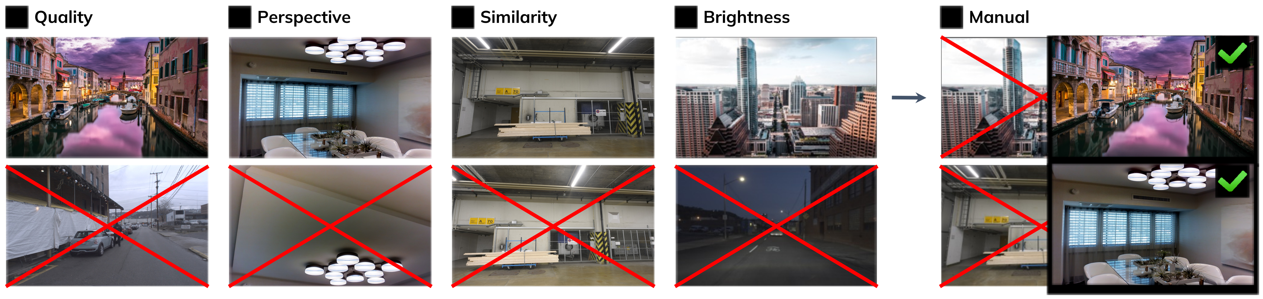
Scene-understanding datasets contain redundant images, unsuitable viewpoints, and narrow fields of view. Filtering selects starting images for the intended generation task rather than sampling the original source distributions uniformly.
Quality.
CLIP-IQA and CLIP Aesthetic remove low-quality candidates. These learned predictors also influence the later evaluation design, so the selected image distribution is shaped by their preferences.
Perspective.
Perspective Fields estimates viewpoint properties. Extreme roll/pitch and narrow fields of view are rejected to favor open, front-facing scenes.
Similarity.
CLIP-based image similarity removes visually redundant examples, including nearby frames from scene datasets.
Brightness.
Images below a brightness threshold are excluded. The prose does not provide numerical thresholds for this or every preceding filtering step.
Human Judgment.
A final manual review removes unsuitable starting views, including examples that automatic quality scoring alone would accept. Figure S1 shows the retained/rejected cases.
B.2 Stylized Image Generation
Each selected photorealistic example receives a generated stylized counterpart from the corresponding caption and a sampled style. These are generated corresponding scenes, not pixel-identical restylings with guaranteed identical geometry.
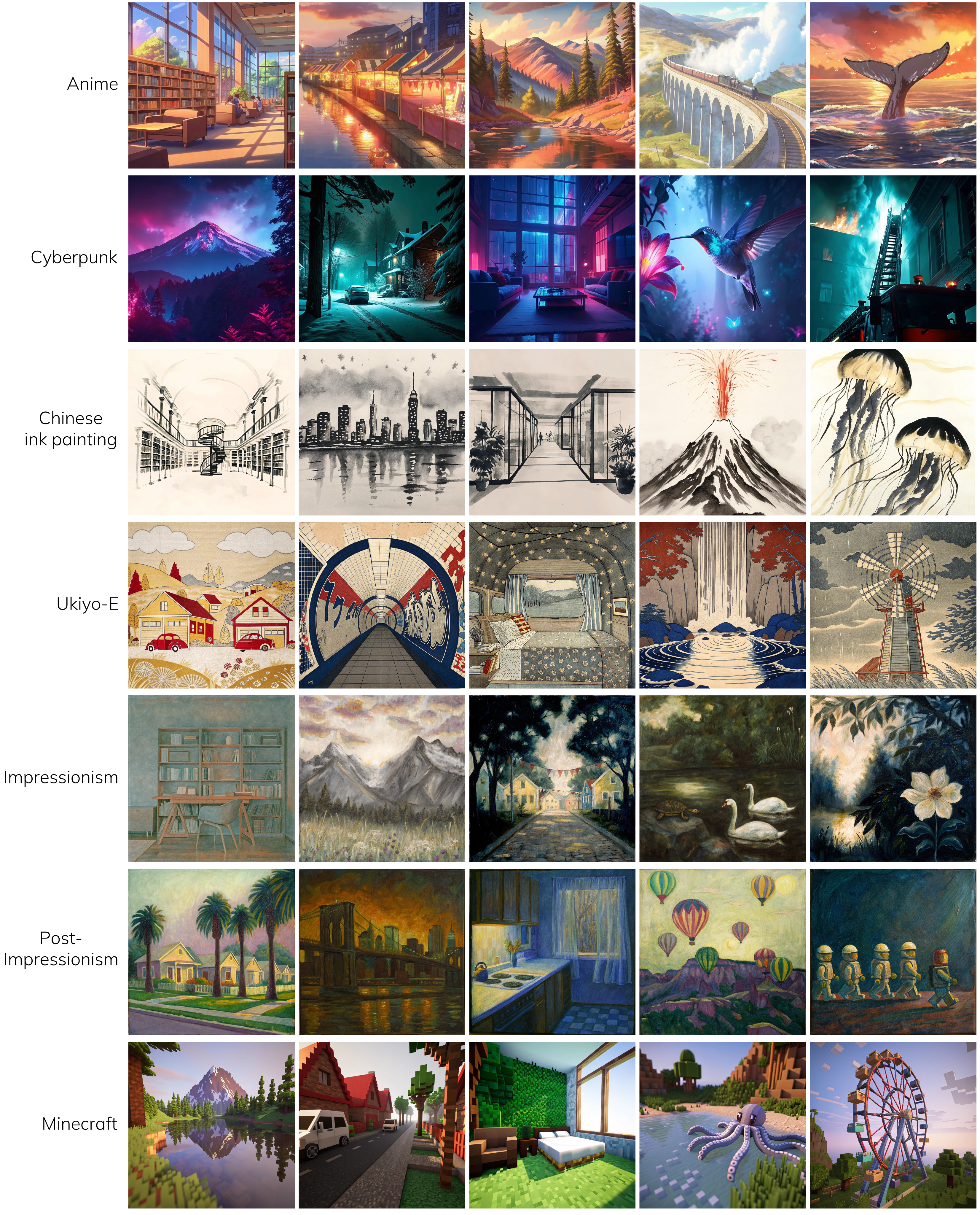
Predefined style sets.
The seven styles are anime, cyberpunk, Chinese ink painting, ukiyo-e, impressionism, post-impressionism, and Minecraft. Figure S2 retains five examples per style.
|
Generated Next-Scene Prompt |
|
Static world generation # Scene 1
# Scene 2
# Scene 3
|
|
Dynamic world generation {“Objects”: [“windmill”, “cloud”, “sea”], “Prompt”: “The windmill blades spin in a circular motion driven by the wind, creating a consistent rotational movement. The clouds drift slowly across the sky, pushed gently by the breeze. The sea surface ripples and undulates, as small waves ripple across its surface.”} |
B.3 Next-Scene Text Prompts Curation
Static prompts ask GPT-4o for one to three prominent entities and a brief interconnected next-scene description; dynamic prompts ask for likely moving objects and their motion. The exact source templates and JSON-like examples are retained below, including their original wording and quotation marks.
The appendix template does not explicitly repeat the main text’s summarized instruction that a new scene must differ from all past scenes. Table S3’s successive prompts can retain a shared armchair while changing the surrounding scene. No stronger uniqueness guarantee is inferred.
“You are an intelligent scene generator. Imaging you are wondering through a sequence of scenes, please tell me what sequentially next scene would you likely to see? You need to generate 1 to 3 most prominent entities in the scene. The scenes are sequentially interconnected, and the entities within the scenes are adapted to match and fit with the scenes. You also have to generate a brief scene description. If needed, you can make reasonable guesses. Please ensure the output is in the following JSON format: {‘Entities’: [‘entity_1’, …], ‘Prompt’: ‘scene description’}.”“You are an intelligent motion dreamer, capable of identifying the objects within an image that can exhibit dynamic motion. I will provide you with an image, and your task is to identify the most prominent object(s) that have the potential for dynamic movement. You also have to briefly describe how the object(s) move. If needed, you can make reasonable guesses. Please ensure the output is in the following JSON format: {’Objects’: [’object_1’, …], ’Prompt’: ’description of how the object(s) move’}.”| Static | Visual Style | Scene Type | Category | # Samples |
| Photorealistic | Indoor | Dining, Living, Passage, Public, Work | ||
| Outdoor | City, Suburb, Aquatic, Terrestrial, Verdant | |||
| Stylized | Indoor | Dining, Living, Passage, Public, Work | ||
| Outdoor | City, Suburb, Aquatic, Terrestrial, Verdant | |||
| Dynamic | Visual Style | Motion Type | # Samples | |
| Photorealistic | Articulated, Deformable, Fluid, Rigid, Multi-Motion | |||
| Stylized | Articulated, Deformable, Fluid, Rigid, Multi-Motion | |||
| # Total Samples | 3000 | |||
Appendix C Additional Details on Metrics
The supplement specifies the estimators and formulas behind each metric, followed by empirical calibration and validation. These definitions make clear which aspects are directly observed and which are inferred by learned models.
C.1 Camera Controllability
DROID-SLAM estimates frame-wise camera poses. Rotation error is the angular difference in degrees; translation error uses a least-squares scale alignment. Errors are combined by geometric mean and averaged over frames/videos.
Scale alignment removes absolute metric-scale evaluation. The printed product also becomes zero if either component error is zero, even when the other is nonzero; the text does not specify an epsilon or alternative handling for that case. The metric therefore should not be read as independently certifying both rotation and translation accuracy.
Equations S1–S2
| (S1) |
| (S2) |
C.2 3D Consistency
DROID-SLAM jointly refines poses and dense depths with bundle adjustment, then measures reprojection residuals over valid co-visible points. This avoids relying only on sparse selected matches.
The residual measures consistency of an estimated reconstruction with the generated frames. The benchmark does not possess a ground-truth 3D world for each generated video, so the source’s “ground truth image” refers to the observed frame used for comparison, not independently verified scene geometry. Tracking quality and valid-point selection can affect the result.
Equation S3
| (S3) |
C.3 Photometric Consistency
Track center-cropped points forward from frame A to B and backward to A, then average their return-distance error over points and frame pairs. Equations S4–S6 retain this definition.
This is optical-flow cycle consistency, not a direct RGB brightness error. It can detect flicker, disappearance, or identity changes, but occlusion and flow-estimator error can also increase it, while a cycle-consistent wrong correspondence can evade it.
Equations S4–S6
| (S4) |
| (S5) |
| (S6) |
C.4 Subjective Quality
Subjective quality is the arithmetic mean of CLIP-IQA+ and CLIP Aesthetic. The combination was selected for the highest agreement among tested predictors in the human study. It estimates human preference under that study’s distribution rather than measuring a universal quality scale.
C.5 Motion Accuracy
SEA-RAFT provides flow magnitude; SAM2 tracks the intended moving-region mask from a supplied first-frame annotation. Motion accuracy subtracts the maximum flow outside the mask from the maximum inside, then averages over frame pairs.
The subtraction is intended to suppress unintended camera motion, but global flow need not be equal inside and outside the mask. The maximum operation is also sensitive to outliers. This checks relative motion placement, not whether the motion’s direction, timing, or physical action matches every semantic detail.
Equation S7
| (S7) |
C.6 Motion Magnitude
Motion magnitude is the median flow magnitude across the image, averaged over frame pairs/videos. It penalizes near-static outputs but can also reward unintended camera/background movement; motion confined to a small object may leave the image-wide median low. It should be interpreted alongside accuracy and smoothness.
C.7 Motion Smoothness
Drop odd-indexed frames, reconstruct them using video frame interpolation, and compare the reconstructions with the original dropped frames using MSE, SSIM, and LPIPS. Normalize the three metrics and average them for smoothness.
The interpolator supplies an estimated reference rather than ground-truth physical motion. Interpolation agreement can favor predictable or small movement and cannot by itself establish that generated dynamics are natural.
C.8 Empirical Bounds
Empirical best/worst values put differently scaled metrics onto a shared range. These reference choices affect aggregate rankings and are part of the benchmark definition.
Empirical bounds for camera controllability.
Zero camera error is the best reference. A fixed-camera sequence supplies the empirical poor-control baseline. This is a calibration choice, not a proven maximum possible error.
Empirical bounds for object controllability.
Object detection success has natural bounds of zero and 100%. These bound the detector-derived success rate, not the correctness of all prompted object properties.
Empirical bounds for 3D consistency, style consistency, and photometric consistency.
Interpolate between randomly sampled unrelated images to construct poor-consistency reference videos. Their errors define empirical maxima for geometry, style, and photometric consistency; zero is the best error. Other failures can fall outside these observed bounds and are clipped during normalization.
Empirical bounds for motion smoothness.
For each prompt, retrieve five semantically similar 3–10-second OpenVid-1M clips. Dropping odd frames and using bilinear interpolation creates the empirical poor-smoothness reference.
The source calls zero the empirical best for smoothness while also listing raw SSIM, whose perfect agreement is one. It does not fully clarify this sign/bound convention; the retained normalization equation distinguishes higher- and lower-is-better metrics.
Empirical bounds for content alignment, subjective quality, motion accuracy, and motion magnitude.
Content alignment, subjective quality, motion accuracy, and motion magnitude use z-score-based calibration chosen so selected-model performance spans roughly 25–75. These scores are relative to that calibration set; changing it can change the scale without changing raw behavior.
C.9 Score Normalization and Mapping
Equation S8 linearly rescales each raw metric between empirical bounds, reverses error metrics, and clips to [0,1] before multiplication by 100. Equal metric weights then produce the two aggregates. Clipping discards distinctions beyond the chosen bounds, and the normalization makes scores benchmark-specific rather than calibrated success probabilities.
Equation S8
| (S8) |
Appendix D Validation with Human Preference
Human comparisons are used to select the quality ensemble, assess selected other metrics, and check sensitivity to image size. The following sections retain the precise agreement rule and the scope of these tests.
Human preference agreement score.
Four hundred participants compare pairs sampled from CogVideoX-I2V, VideoCrafter1-I2V, DynamiCrafter, WonderJourney, and InvisibleStitch. For each pair, a metric receives the fraction of people preferring its selected winner, or 0.5 for a tie; final agreement averages across pairs.
This is a probabilistic pairwise agreement score, not a correlation coefficient despite Table S5’s heading. The question asks which video has higher overall quality. The text does not describe a separate held-out study for ensemble selection and validation or report uncertainty intervals.
Agreement results on subjective quality.
CLIP-IQA+ plus CLIP Aesthetic reaches 0.637 agreement, compared with 0.628 for CLIP Aesthetic alone and a 0.772 majority-vote upper bound. Its measured advantage is small; no confidence interval or significance test is supplied.
Agreement results on other metrics.
Table S6 compares score buckets centered at 30, 60, and 90 with width ±5 for camera control, object control, 3D consistency, photometric consistency, and motion magnitude. Higher-score examples are preferred in 71.2–97.3% of the listed comparisons.
This supports separation of widely spaced buckets for five dimensions. It does not validate every metric, fine ranking between near-tied models, or a task-specific causal interpretation of overall-quality preferences.
Robustness against different resolutions and aspect ratios.
EasyAnimate outputs at 1344×768 are center-cropped/resized to 256×256 and rescored. Most differences are small, but motion magnitude changes from 37.76 to 36.90: 0.86, exceeding the prose’s stated maximum of 0.83. All original table values remain intact.
The test concerns one generator and one transformation, not every resolution/aspect ratio or output modality. Some Table S7 original-resolution scores also differ from EasyAnimate’s main-table scores; the text does not explain that difference.
| Metric | Correlation |
| CLIP-IQA | 0.596 |
| CLIP-IQA+ | 0.602 |
| QAlign Quality | 0.581 |
| QAlign Video Quality | 0.571 |
| MUSIQ | 0.530 |
| CLIP Aesthetic | 0.628 |
| QAlign Aesthetic | 0.479 |
| QAlign Video Aesthetic | 0.556 |
| CLIP-IQA+ & QAlign Quality | 0.582 |
| CLIP Aesthetic & QAlign Video Aesthetic | 0.629 |
| CLIP-IQA+ & CLIP Aesthetic | 0.637 |
| Upper Bound | 0.772 |
|
Cam Ctrl
|
Obj Ctrl
|
3D Consist
|
Photo Consist
|
Motion Mag
| |
| over | 71.2% | 96.3% | 91.7% | 91.6% | 91.8% |
| over | 73.5% | 87.7% | 97.3% | 95.1% | 76.2% |
|
Res.
|
Cam
Ctrl
|
Obj
Ctrl
|
Content
Align
|
Consist
|
Photo
Consist
|
Style
Consist
|
Subject
Qual
|
Motion
Acc
|
Motion
Mag
|
Motion
Smooth
|
| 1344×768 | 25.72 | 54.50 | 49.81 | 67.29 | 46.65 | 73.05 | 49.66 | 75.00 | 37.76 | 40.32 |
| 256×256 | 25.69 | 53.78 | 50.32 | 67.41 | 47.06 | 73.88 | 48.99 | 74.89 | 36.90 | 39.62 |
Appendix E Further Visualization
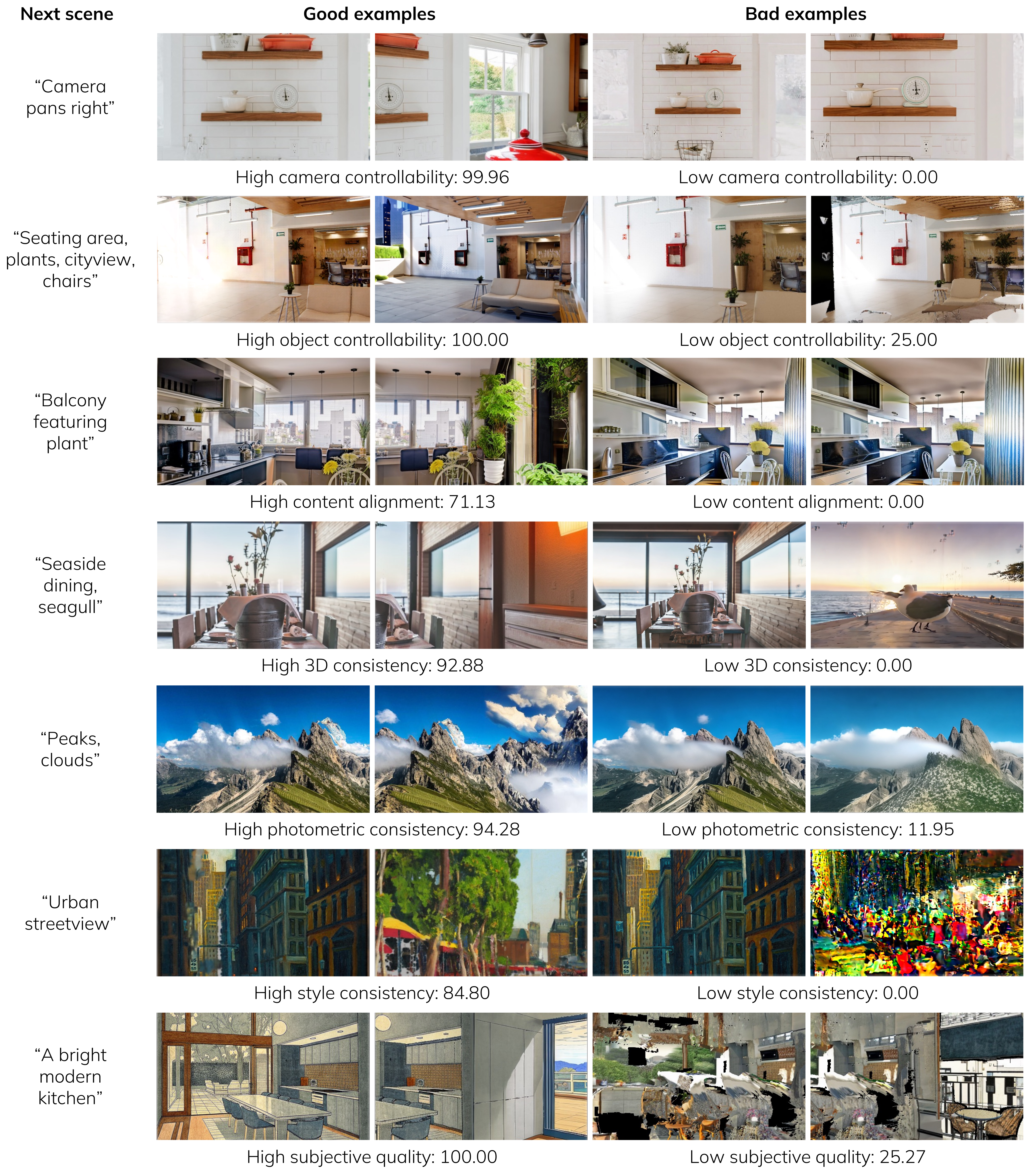
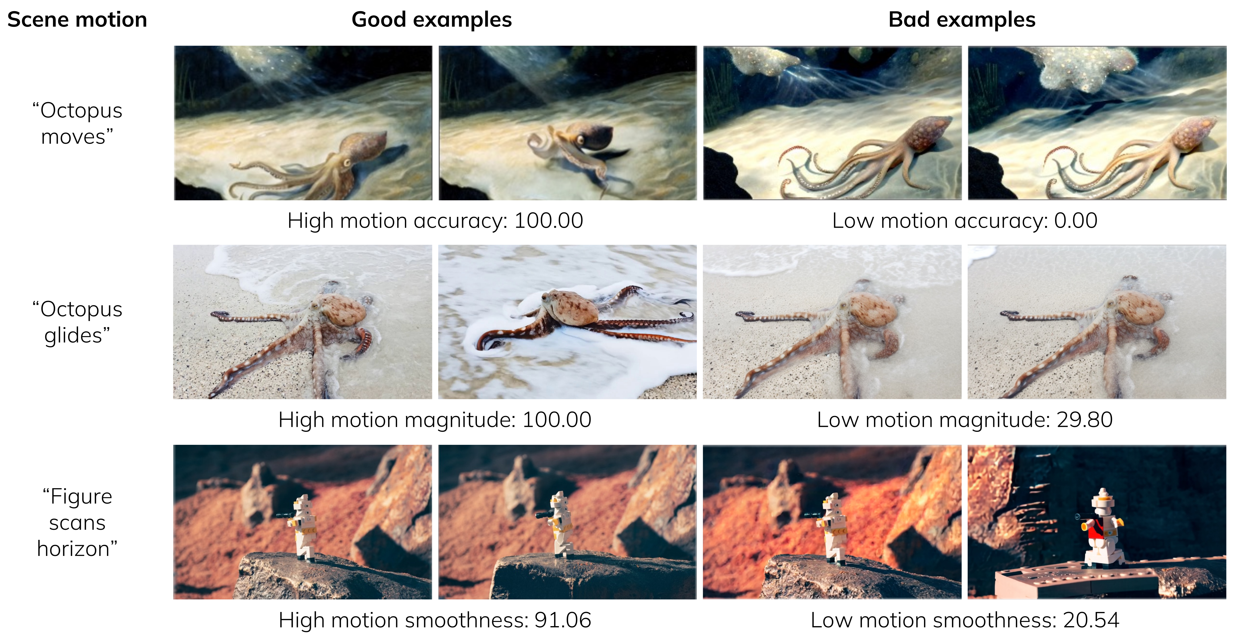
Figures S3 and S4 show good/bad examples for all ten metrics, retaining the prompted content, rendered frames, and score labels. Figures S5 and S6 plot selected dynamic and static model profiles. The HTML prose repeats the S6 reference for both charts; the actual captions distinguish them.
These profiles make trade-offs visible: video models lack precise camera control, large motion can be jittery, and 3D methods can preserve geometry without maximizing aesthetic preference. Ten separately reported dimensions are useful diagnostics, but the experiments do not establish statistical independence among them.