At a glance
This study varies simulated and real demonstration amounts, their sampling ratio, and domain differences while training diffusion policies for image-based planar pushing. Simulated data substantially helps when real demonstrations are scarce, but gains plateau and additional target-domain data raises that ceiling. Controlled simulation experiments show that physics differences matter and that policies may need to recognize their domain to select compatible actions. The evidence spans more than fifty physical policies and 250 simulated policies, but concerns one task family and best-checkpoint evaluations.
I Introduction
Simulation offers inexpensive demonstrations, while real data captures deployment physics and behavior. The paper asks how to combine them effectively rather than eliminate the real-data requirement. Its main observations are low-data benefits, sensitivity to the sampling mixture, diminishing simulation returns, and a role for domain identity when actions differ across environments. The strongest conclusions are empirical trends within planar pushing, not universal prescriptions for every robot task.
II Related Work
Related work motivates scalable simulation data generation and joint training across domains.
II- 1 Data Generation in Simulation
Simulation generation, environment reconstruction, and planning can produce robot-specific trajectories at scale. This study analyzes how their resulting data complements real demonstrations, rather than proposing a new simulator or collection method.
II- 2 Sim2real Transfer vs Sim-and-Real Cotraining
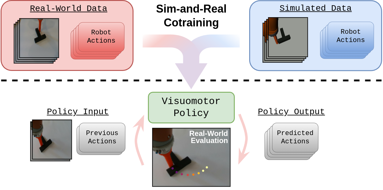
Cotraining samples real and simulated examples throughout behavior cloning. It differs from training only in simulation followed by deployment or real-only fine-tuning. The setting is one instance of multi-domain learning, with controllable visual, physical, and demonstration-policy differences.
III Preliminaries
The experimental setup combines a shared diffusion-policy architecture with matching planar-pushing observation and action interfaces.
III-A Cotraining Problem Formulation and Notation
A dataset contains observation–action trajectories from a source simulator and a real target environment. Joint behavior cloning is evaluated by binary task success in the target domain. Later simulator-to-simulator studies replace the real target with a distinct controlled environment and should be interpreted separately.
III-B Diffusion Policy
The policy uses Diffusion Policy [14] with a ResNet18 image encoder and U-Net denoiser, trained end to end. It predicts an action horizon conditioned on recent images and pusher state by learning to remove noise from demonstrations. The original denoising loss is retained.
Equation 1
| (1) |
III-C Planar-Pushing From Pixels
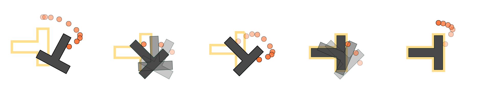
A cylindrical pusher moves a slider across a flat surface to a goal pose. Images replace direct slider-state observations, requiring visual control and contact handling. The narrow task makes large sweeps feasible while limiting conclusions about grasping, semantics, or broader manipulation.
III-D Data Collection
Humans teleoperate real demonstrations, while an optimization-based contact planner [35] produces simulated trajectories that are replayed and rendered in Drake [38]. More than 25,000 unique trajectories are generated without retuning planner costs. Because planned and human actions differ, the datasets contain a behavior gap as well as visual and physical gaps.
Both domains model a KUKA iiwa with fixed-height/orientation pushing. Actions are target planar pusher positions; inputs include pusher pose plus overhead and wrist RGB views. This common interface controls embodiment differences in the principal experiment.
IV Real World Experiments
Physical experiments sweep real-data amount, simulated-data amount, and the probability of sampling a real example, then compare joint training with sequential fine-tuning.
IV-A Experimental Setup
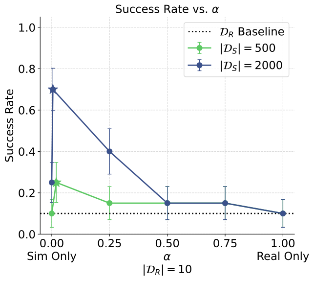
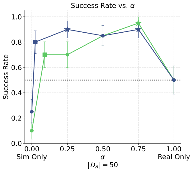
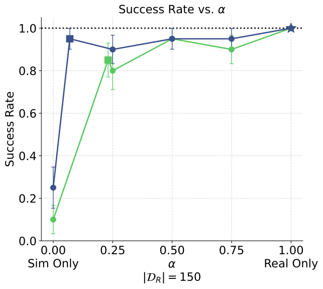
The real sampling probability α weights the real and simulated cloning losses. Sweeps use 10, 50, or 150 real demonstrations; 500 or 2,000 simulated demonstrations; and pure-domain, natural-concatenation, or deliberately reweighted mixtures. Real performance is reported for the best checkpoint on twenty fixed initial conditions. Error bars describe trial uncertainty for that checkpoint and omit variation across training seeds; selection among checkpoints and mixtures also matters when interpreting the best reported scores.
Equation 2
| (2) |
IV-B Does Cotraining Improve Performance?
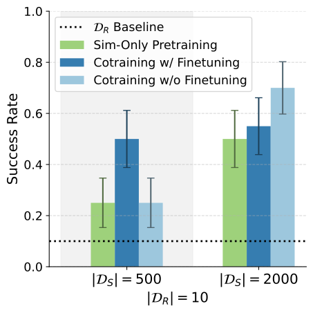
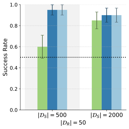
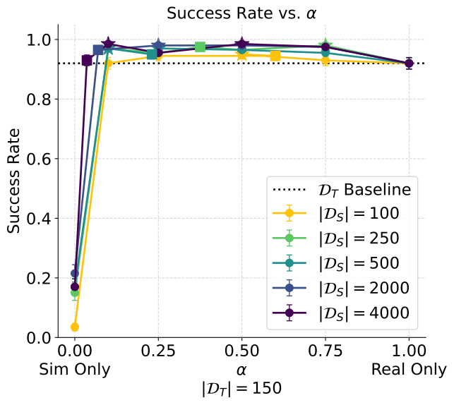
With ten real demonstrations, the best mixture increases success from 2/20 to 14/20; with fifty, it increases 10/20 to 19/20. With 150 real demonstrations, the real-only policy already obtains 20/20, and small cotraining decreases lie within the displayed trial uncertainty. A perfect twenty-trial result does not establish a universally successful policy.
IV-C The Effect of α , | 𝒟 R | , and | 𝒟 S | on Cotraining
The effects of mixture, real-data scale, and simulated-data scale interact, so no single fixed ratio is established as universally optimal.
IV-C 1 Effect of α
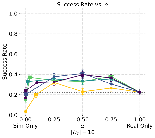
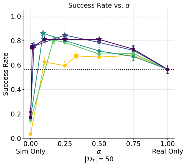
Performance is especially sensitive to α with only ten real demonstrations. Even a small real fraction can greatly outperform simulated-only training. Larger real datasets can tolerate more weight on the real loss, although added simulation weakens that trend.
IV-C 2 Effect of | 𝒟 R |
The largest relative benefits occur when the real-only baseline is weak. Ten real demonstrations still leave substantial failures after cotraining, whereas fifty plus simulation can approach the high-data result on this task. The suggestion that other tasks may remain data-limited at much larger counts is a motivation for further study, not measured here.
IV-C 3 Effect of | 𝒟 S |
Increasing simulated data from 500 to 2,000 examples improves or maintains the tested physical results and often reduces sensitivity to α. The larger controlled simulation sweep tests where this improvement saturates.
IV-D Finetuning Comparison
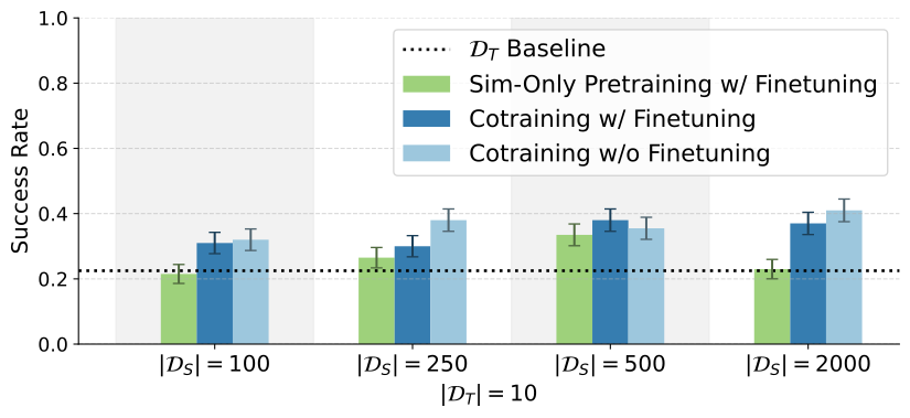
Joint data mixing outperforms simulated-only pretraining followed by real-only fine-tuning in these comparisons. Further real-only fine-tuning of an already cotrained model does not consistently help and may overfit the small real dataset. The result concerns the tested single-task setup, not every multi-task fine-tuning schedule.
V Simulation Experiments
A second simulator acts as the target environment, enabling 200-trial evaluations and controlled variation of domain gaps. This supplies more precise comparisons but remains an approximation to physical transfer.
V-A Sim-and-Sim Setup
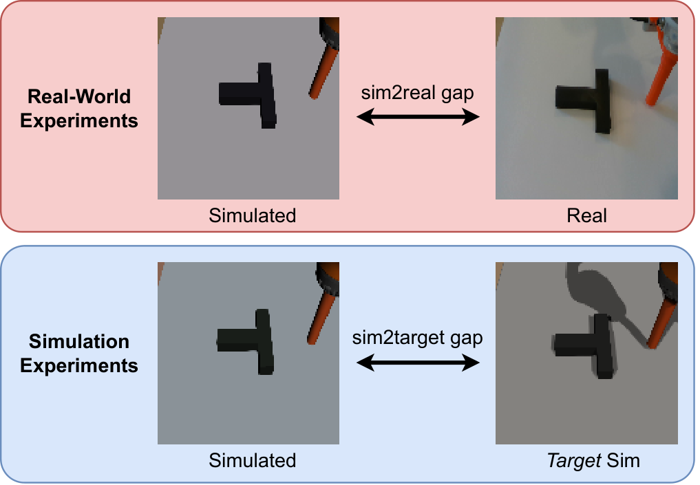
The source uses quasistatic planned behavior and simple rendering; the target uses Drake physics, human teleoperation, warmer lighting, and shadows. These differences mimic the physical study along physics, appearance, and behavior axes. Each policy is evaluated for up to 200 target-simulator trials rather than twenty hardware trials.
| Gap | Simulation | Real World | Target Sim |
|---|---|---|---|
| Visual | white light, camera & color offset | natural light, shadows | warm light, shadows |
| Physics | Quasistatic | Real physics | Drake physics |
| Action | Motion planning | Human teleop | Human teleop |
V-B Single-Task Cotraining Asymptotes
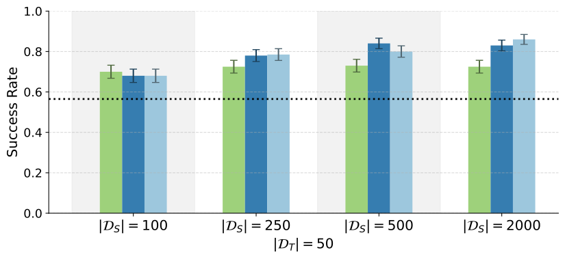
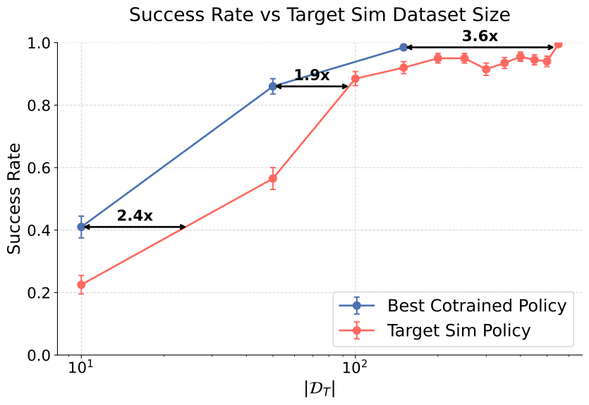
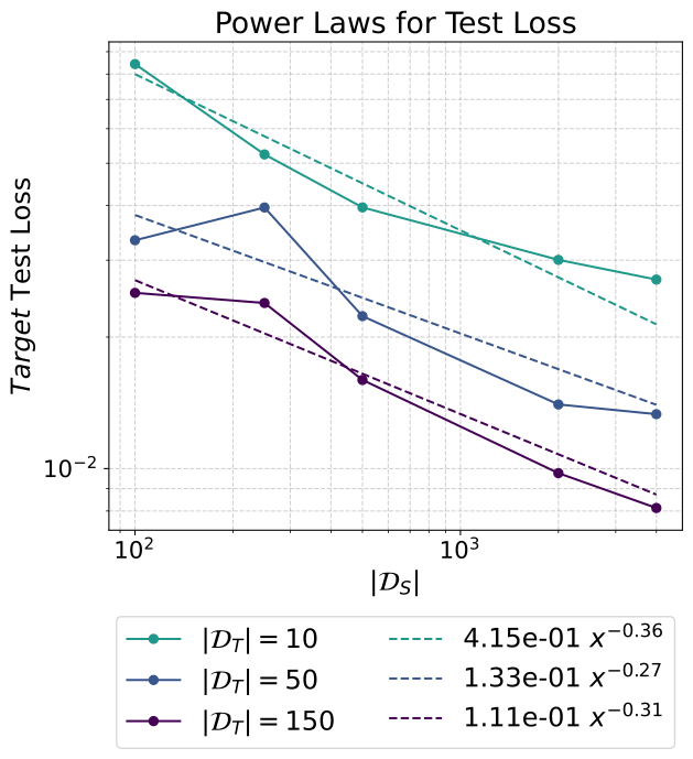
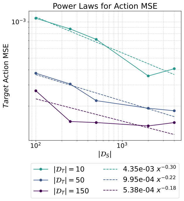
Source datasets range from 100 to 4,000 trajectories, with 10, 50, or 150 target demonstrations. Simulation gains eventually plateau, and more target data raises the plateau. In this setup, the best mixtures roughly match adding two to three times as much target-only data. Optimal real/target fractions differ from the physical experiment, underscoring dependence on the actual domain gap.
V-C Distribution Shift Experiments
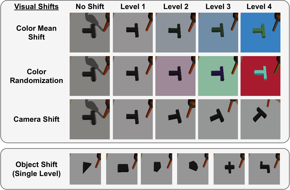
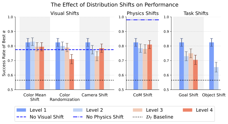
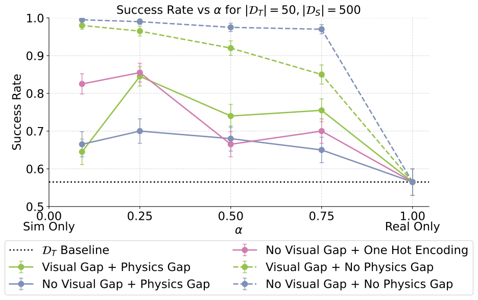
One shift is varied at a time while keeping fifty target and 2,000 source demonstrations. The six interventions change color mean, color randomization, camera pose, center of mass, goal pose, or object shape. The reported curve selects the best sampling mixture for each setting. Physical, visual, and task shifts use different units and are not normalized to a common severity scale.
Larger gaps generally harm performance. Removing the baseline physics gap produces a reported 15.5-percentage-point success increase, supporting the importance of contact dynamics here. Yet removing every visual difference while retaining different physics slightly hurts: identical appearances conceal which action dynamics apply. Removing both gaps reverses that effect. This supports matching physics and retaining useful domain information, rather than a general claim that worse rendering is desirable.
VI How does cotraining succeed?
The mechanism analysis asks how policies preserve domain-specific behavior while benefiting from a second domain’s data.
VI-A Sim-and-Real Discernability
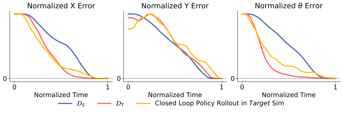
Binary probes classify the environment perfectly from observation embeddings and at 74.2–93% from final activations in the listed policies. This demonstrates retained domain information, though probing alone does not establish causal necessity. The stronger intervention removes appearance differences and then restores identity through a one-hot domain label: that recovers performance when physics differs. With matched physics, eliminating visual differences instead helps.
| Policy | Binary Probe Location | |||
|---|---|---|---|---|
| Observation Embedding | Final Activation | |||
| 50 | 500 | 0.75 | 100% | 74.2% |
| 50 | 2000 | 0.75 | 100% | 89% |
| 10 | 500 | 0.75 | 100% | 84% |
| 10 | 2000 | 5e-3 | 100% | 93% |
VI-B Mechanisms For Positive Transfer in Cotraining
The paper considers coverage of missing states and reductions in target-domain predictive loss as explanations for positive transfer.
VI-B 1 Coverage
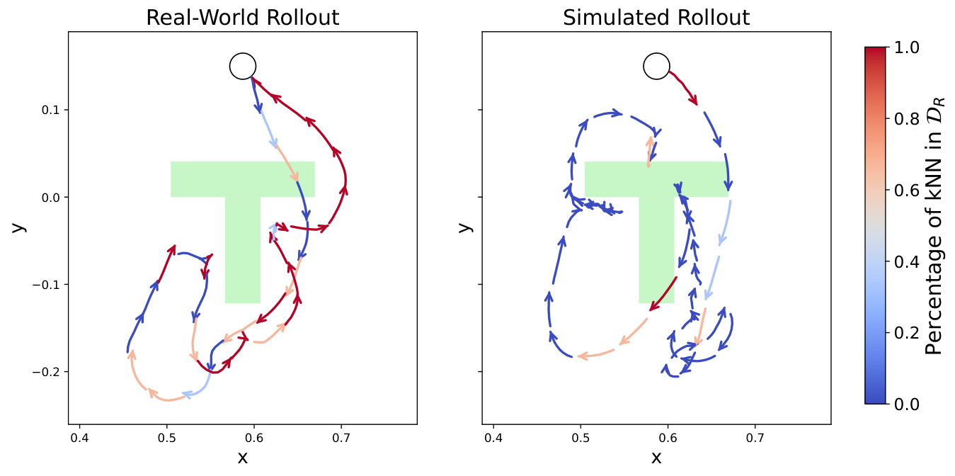
A nearest-neighbor diagnostic compares each predicted action chunk and observation embedding with training examples from both domains. Physical rollouts mostly resemble real examples, interspersed with simulated neighbors; simulated rollouts show the reverse. This is consistent with simulation filling data gaps. Nearest-neighbor membership is a heuristic attribution, however, and cannot prove which training examples causally produced an action.
VI-B 2 Power Laws
On held-out target-simulator data, fitted denoising loss scales approximately with source count to −0.332 and target count to −0.397; action error exponents are −0.285 and −0.587. Fits have R² of 0.945 and 0.975. These describe predictive losses over the tested range, not a universal success-rate scaling law, and action error begins to flatten at large source counts. The test set is not used for training or checkpoint selection in this analysis.
Equation 3
| (3) | |||
VII Ablations
Two alternative objectives test whether explicitly amplifying domain-specific behavior or aligning internal domain representations improves the baseline.
VII-A Classifier-Free Guidance Ablation
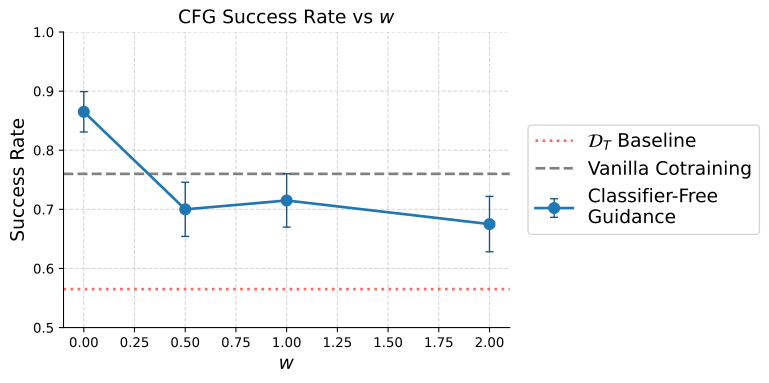
Adding a one-hot environment label and sampling normally improves the tested setting. Increasing classifier-free guidance strength beyond zero, which amplifies the conditional–unconditional action difference, does not improve over vanilla cotraining. Domain identification and exaggerated domain-specific action predictions therefore have different empirical effects.
Equation 4
| (4) |
VII-B Alternative Cotraining Loss
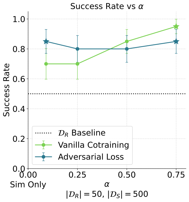
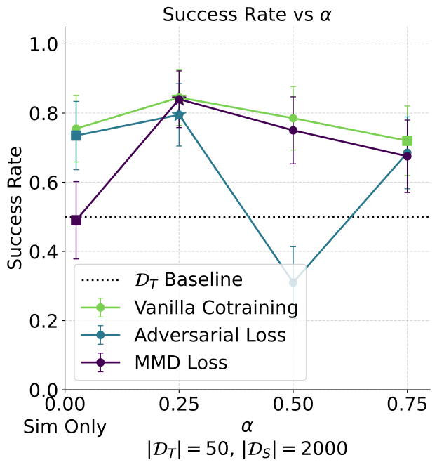
The alternative loss combines cloning with a penalty on differences between simulated and real representation distributions. One version uses an adversarial classifier; another uses maximum mean discrepancy with Gaussian kernels. Neither reliably beats vanilla cotraining. The adversarial version is unstable and is not swept as extensively as the discrepancy coefficient. These negative results limit the tested formulations, while leaving other representation objectives open.
Equations 5–6
| (5) |
| (6) | ||||
VIII Limitations
All evaluations use image-based planar pushing, one diffusion-policy family, and the chosen planner/teleoperation sources. Extending to multiple tasks, different imitation methods, and different synthetic-data pipelines is necessary before treating the trends as general rules. The narrow scope is deliberate and enables the extensive sweeps.
IX Conclusion
Joint training can make simulated demonstrations useful even when target dynamics and behavior differ. The study supports tuning domain mixture, retaining some target examples, and evaluating how physics and domain identity interact. Simulation scaling helps within limits; target-data scarcity remains a constraint.
-A Real-World Evaluation
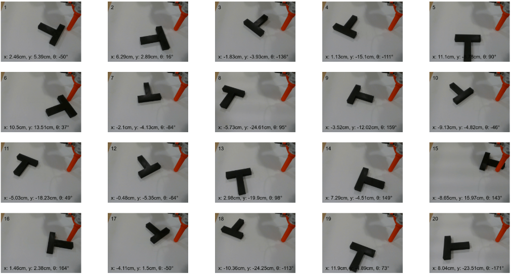
Hardware evaluation uses twenty fixed initial conditions and a 90-second timeout. A trial succeeds when a human judge would not readjust the final slider pose; it does not use the numerical pose tolerance of the simulation test. Results select the best saved checkpoint and show binomial standard errors, which do not capture training randomness or checkpoint-selection uncertainty. Figure 17 retains all initial conditions and the successful-demonstration overlay.
-B Simulation Evaluation
Simulation success requires returning the pusher to its default position and placing the slider within 1.5 cm and 3.5° of the goal within 75 seconds. Up to 200 trials evaluate saved checkpoints, with a Bayesian procedure discarding poor checkpoints early. The reported best-checkpoint scores therefore use a selection procedure rather than one prespecified final model.
-C Training Details
The same architecture and approximately equal optimizer-step budgets are used across comparisons, after a small hyperparameter sweep. Four or five checkpoints are saved. Fine-tuning reduces learning rate tenfold, and its best checkpoint is reported. The released configurations provide detailed per-run settings.