Overview
This edition follows the main paper and complete supplement of arXiv v2. It retains all original figures, tables, equations, and references, with the experimental scope and source inconsistencies explained alongside the condensed text.
At a glance
Gaussian Atlas organizes the attributes of a 3D Gaussian object into a dense 2D grid, enabling a pretrained image diffusion denoiser to generate 3D objects from text. GaussianVerse supplies 205,737 fitted objects for training. The atlas uses optimal transport to impose a consistent ordering, while a modified denoiser predicts Gaussian attributes directly without an image autoencoder.
The reported model improves text–render alignment and pairwise user preference over the tested Gaussian-generation baselines, using 16,384 Gaussians per object. This is a transfer of pretrained image-model weights into a system trained on substantial 3D supervision, not 3D generation without 3D data. Project materials accompany the paper.
1 Introduction
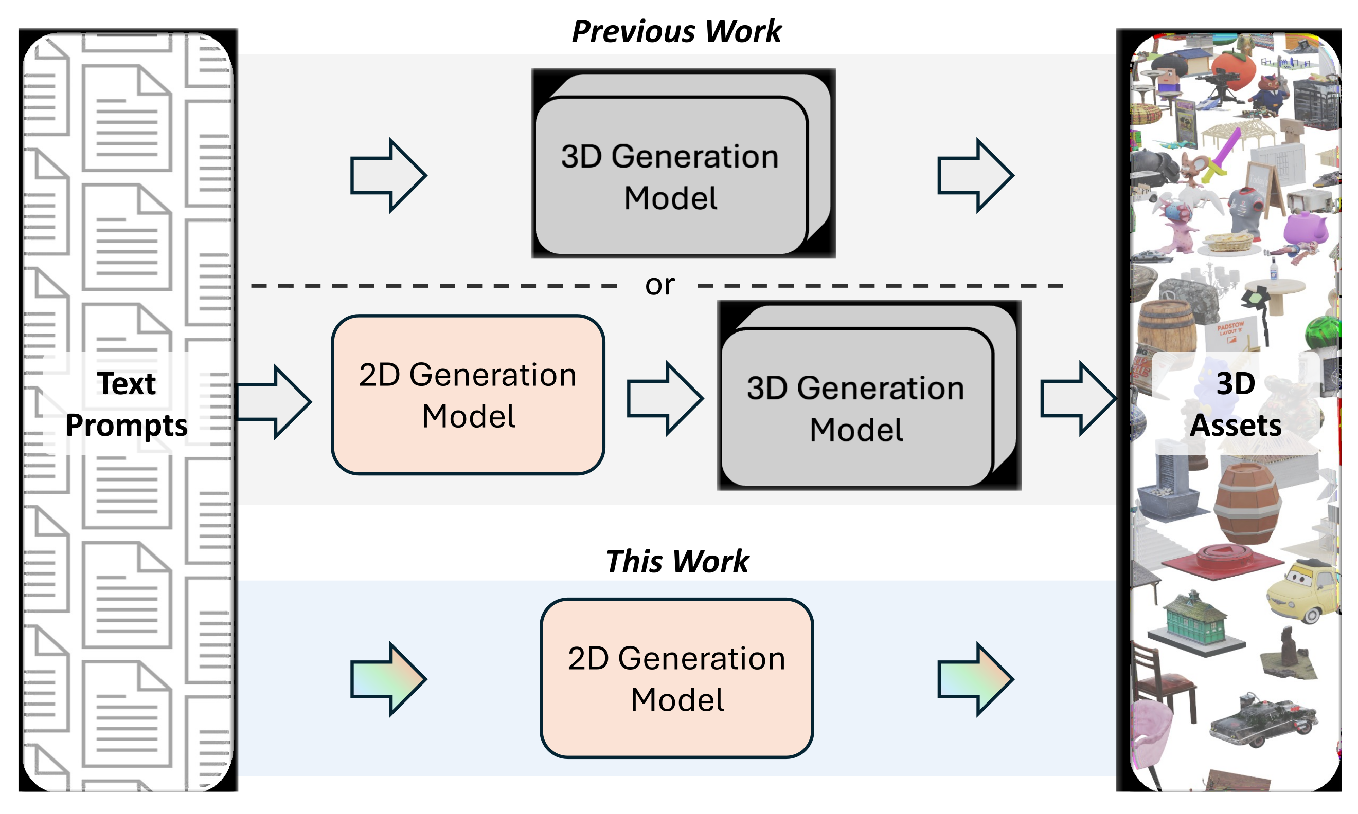
Strong 2D diffusion models benefit from much larger training corpora than 3D generators. Gaussian Atlas asks whether a 3D representation can be made compatible with a pretrained 2D denoiser rather than training a new 3D model from scratch.
The contribution has three parts: a large collection of Gaussian-fitted objects, a deterministic sphere-to-plane atlas construction, and direct fine-tuning of the denoiser on normalized Gaussian attributes. This differs from using a frozen image model only to score or initialize a separate reconstruction pipeline.
The representation retains original Gaussian position offsets and other attributes; the grid is not simply a rendered image or a projection that discards depth. Its usefulness is supported by the tested generation and initialization comparisons, not a guarantee that arbitrary 3D structure is perfectly preserved under flattening.
2 Related Work
Depth-estimation methods such as Marigold show that image diffusion priors can support new output modalities. Gaussian Atlas follows this adaptation idea for 3D generation, while bypassing the pretrained image autoencoder because its reconstruction error damages Gaussian attributes.
Gaussian generators such as GaussianCube and GVGen organize fitted primitives for diffusion. Triplane methods offer another 2D-like representation, and systems such as Splatter Image predict pixel-aligned Gaussians from images. Here the atlas predicts all Gaussian attributes using the architecture and initial weights of a 2D diffusion denoiser.
Related approaches differ in conditioning, representation, and available implementations. Omages is class-conditioned rather than a direct text-to-3D comparison; the paper could not compare directly with PI3D, HexaGen3D, or GIMDiffusion implementations. The experiments therefore do not establish superiority over every approach discussed.
3 GaussianVerse
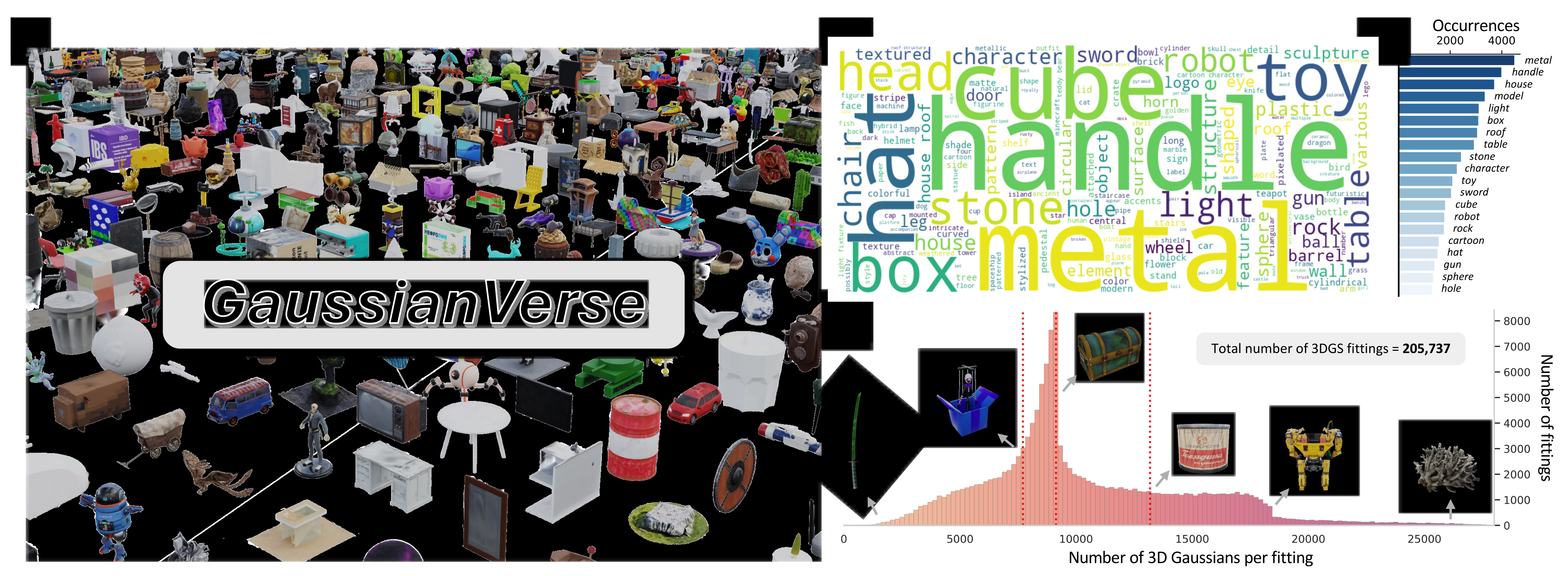
GaussianVerse contains 205,737 fitted 3D objects sampled from Sketchfab under Creative Commons licenses. Fits use existing multiview renders and captions. Nine of ten rendering categories are retained after excluding a lower-quality category. The dataset averages 10,435±4,453 valid Gaussians per object and costs more than 3.8 A100 GPU-years to construct.
A Gaussian carries position, color, opacity, scale, and rotation. Front-to-back alpha compositing produces the image in Equation 1. The preliminaries describe a three-component rotation, but the actual atlas implementation later uses a four-component quaternion; the channel construction below follows that implementation.
Fitting starts from Scaffold-GS with view-dependent attribute inputs removed. After densification, excess Gaussians are pruned using averaged opacity and anchor-visibility rankings, with a cap of 192²=36,864 valid Gaussians. Adaptive counts avoid forcing simple and complex objects to use the same number; this heuristic does not certify a globally minimal representation.
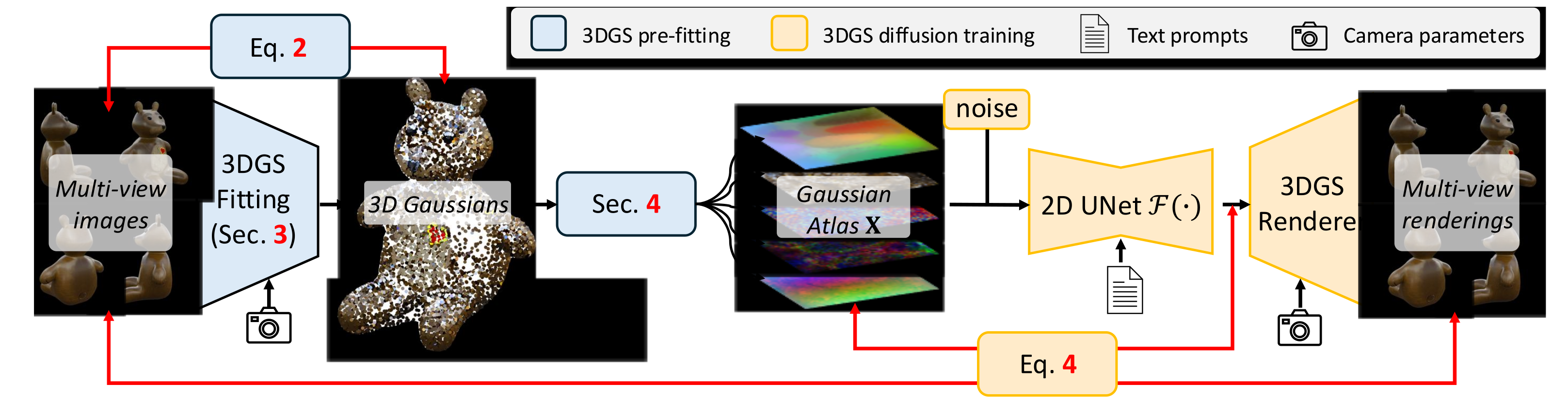
Equation 2 combines RGB L1, negated structural similarity, perceptual loss, and scale regularization. Perceptual loss nearly doubles fitting cost but improves rendering quality. Each object uses about 20,000 fitting steps, roughly ten minutes on the stated A100 setup. This expensive preprocessing is separate from the fast final sampling time.
| # Gaussians per fitting | Total # fittings | Compute time |
| 10,4354,453 | 205,737 | 3.8 GPU Years |
Equation 1
| (1) |
Equation 2
| (2) |
4 Formulating 3D Gaussians as 2D Atlas
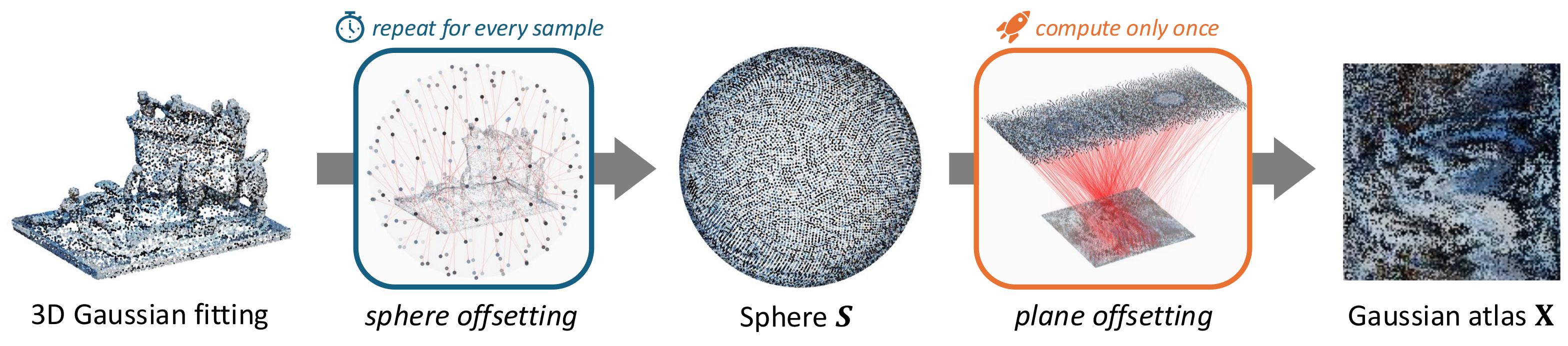
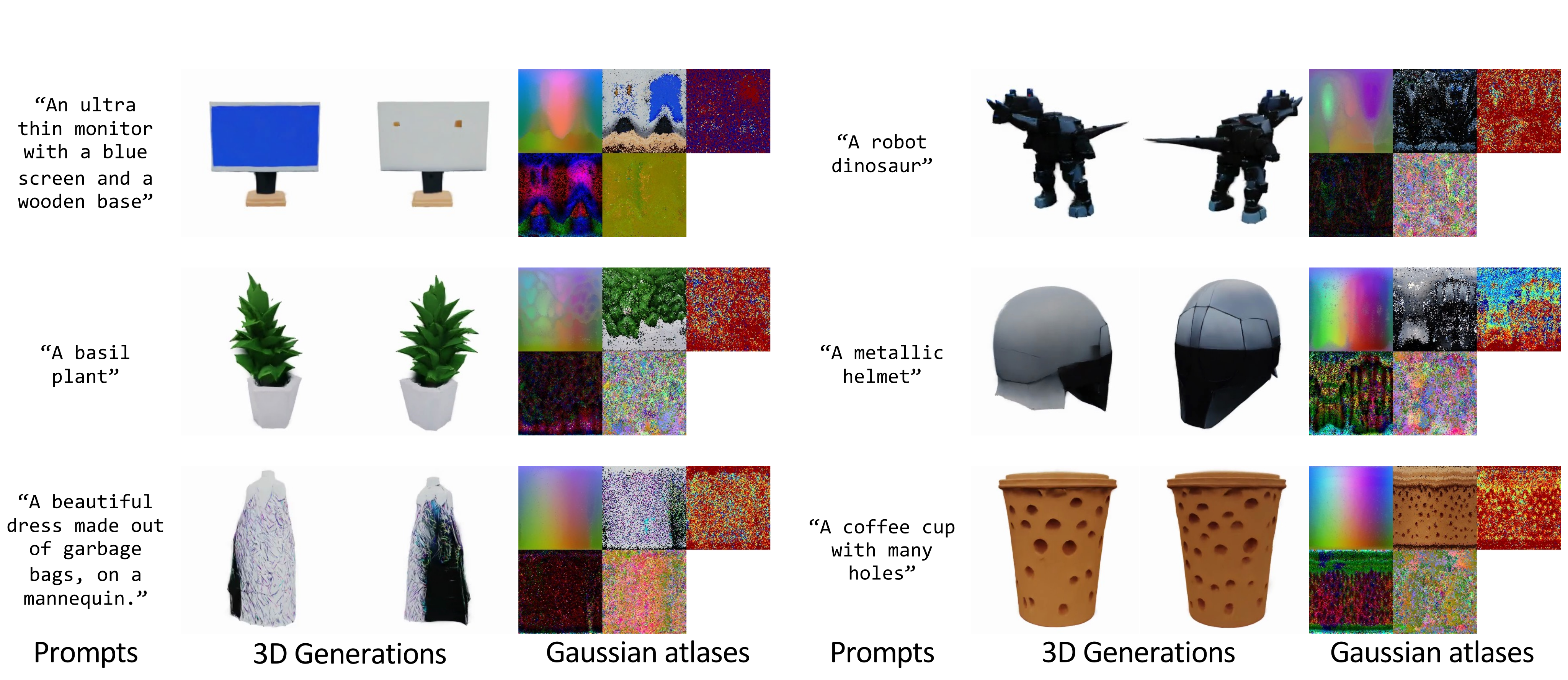
Atlas construction first assigns each object’s Gaussians to points on a shared unit sphere using optimal transport. It stores position offsets from those assigned sphere points. Equirectangular projection flattens the sphere, and a second transport assigns flattened points to a regular square grid.
The per-object sphere assignment is recomputed; the sphere-to-grid assignment is shared and computed once. This consistent indexing is intended to create learnable spatial patterns across different objects. The atlas preserves the Gaussian attributes rather than treating the projected position alone as the 3D representation.
In the implementation, N denotes the total number of slots: 16,384 gives a 128×128 grid. The text’s occasional N-by-N wording should not be read as 16,384 slots on each side. Equirectangular boundaries and rearrangement can still disturb neighborhoods; the observed absence of seams in examples is empirical rather than a topological guarantee.
5 2D Diffusion for 3D Gaussian Generation
A standard latent diffusion model uses an image autoencoder and a denoising UNet. Gaussian Atlas removes the autoencoder, normalizes atlas values using dataset-wide per-pixel means and standard deviations, and fine-tunes the denoiser directly. Matching these moments helps interface the data with the model but does not make the full atlas distribution identical to natural-image latents.
Position, albedo, and scale each have three channels; opacity is appended to each, giving three four-channel groups. A four-channel rotation quaternion provides the fourth group. The denoiser’s input layer is repeated four times and its output layer adapted to predict a 128×128×16 atlas. Rendering averages the three predicted opacity copies.
Equation 3 is the paper’s printed diffusion objective and velocity notation. Its unusual gradient-like symbols are retained rather than reinterpreted as a new differentiation procedure. Equation 4 adds rendered RGB L1, opacity-mask L1, and perceptual losses, connecting attribute denoising to visible object quality.
Equation 3
| (3) |
Equation 4
| (4) |
6 Experiments
Training uses about 130,000 atlases, matching the comparison with GaussianCube rather than using all 205,737 dataset objects. The denoiser starts from a pretrained latent diffusion model and uses CLIP text embeddings, 20% text dropout, AdamW at 5×10⁻⁵, batch size 64, an exponential moving average, and mixed precision. Training runs for one million steps on eight A100 GPUs.
Inference samples Gaussian-atlas noise with DPM-Solver++ and classifier-free guidance 3.5. The paper reports generation and rendering in under five seconds; that speed excludes fitting the training dataset, atlas construction, and model training.
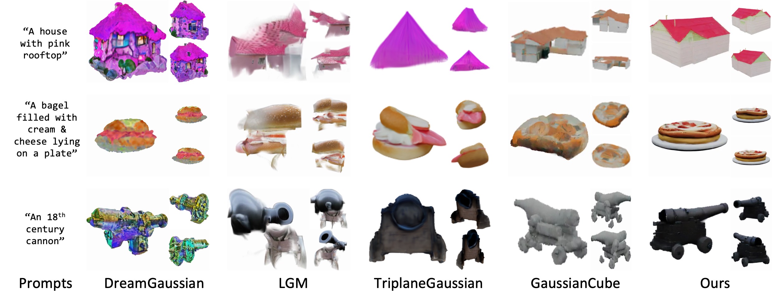
Evaluation uses 100 diverse prompts and ten random rendered views per generated object, scored with CLIP similarity and a visual-question-answering metric. These assess alignment of rendered appearances with text, not ground-truth 3D geometry. DreamGaussian, LGM, TriplaneGaussian, and GaussianCube are the main comparisons; LGM and TriplaneGaussian receive MVDream-generated images as input.
| Methods | CLIP score | VQA score | # Gaussians |
| DreamGaussian [46] | 20.52 | 0.37 | 40K |
| LGM [47] | 20.28 | 0.35 | 66K |
| TriplaneGaussian [60] | 21.10 | 0.46 | 16K |
| GaussianCube [57] | 22.31 | 0.52 | 33K |
| GaussianAtlas (Ours) | 23.20 | 0.61 | 16K |
6.1 Results
Table 2 reports CLIP 23.20 and VQA 0.61, versus GaussianCube’s 22.31 and 0.52. The VQA difference is 0.09 absolute, approximately 17% relative. Gaussian Atlas uses 16K Gaussians versus GaussianCube’s 33K, about half; it ties TriplaneGaussian’s listed 16K rather than uniquely minimizing the count.
Qualitative examples show improved prompt details and more coherent objects in the selected cases. They do not measure failure frequency across all possible prompts. The table caption calls these comparisons qualitative, but its entries are quantitative scores and counts.
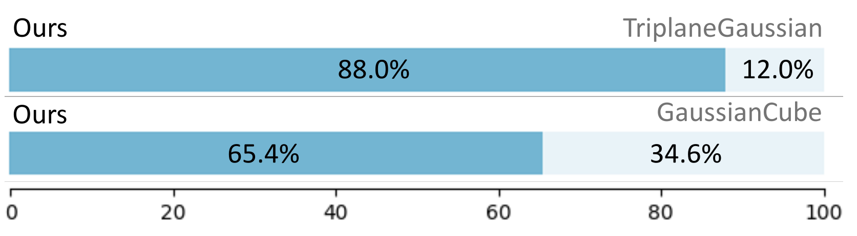
A pairwise preference study collected more than 2,500 valid responses and reports 65.4% preference over GaussianCube and 88.0% over TriplaneGaussian. Responses are not necessarily distinct participants. The study was conducted by Stanford researchers; participant-level independence, demographics, and confidence intervals are not reported here.
6.2 Discussions and Ablations
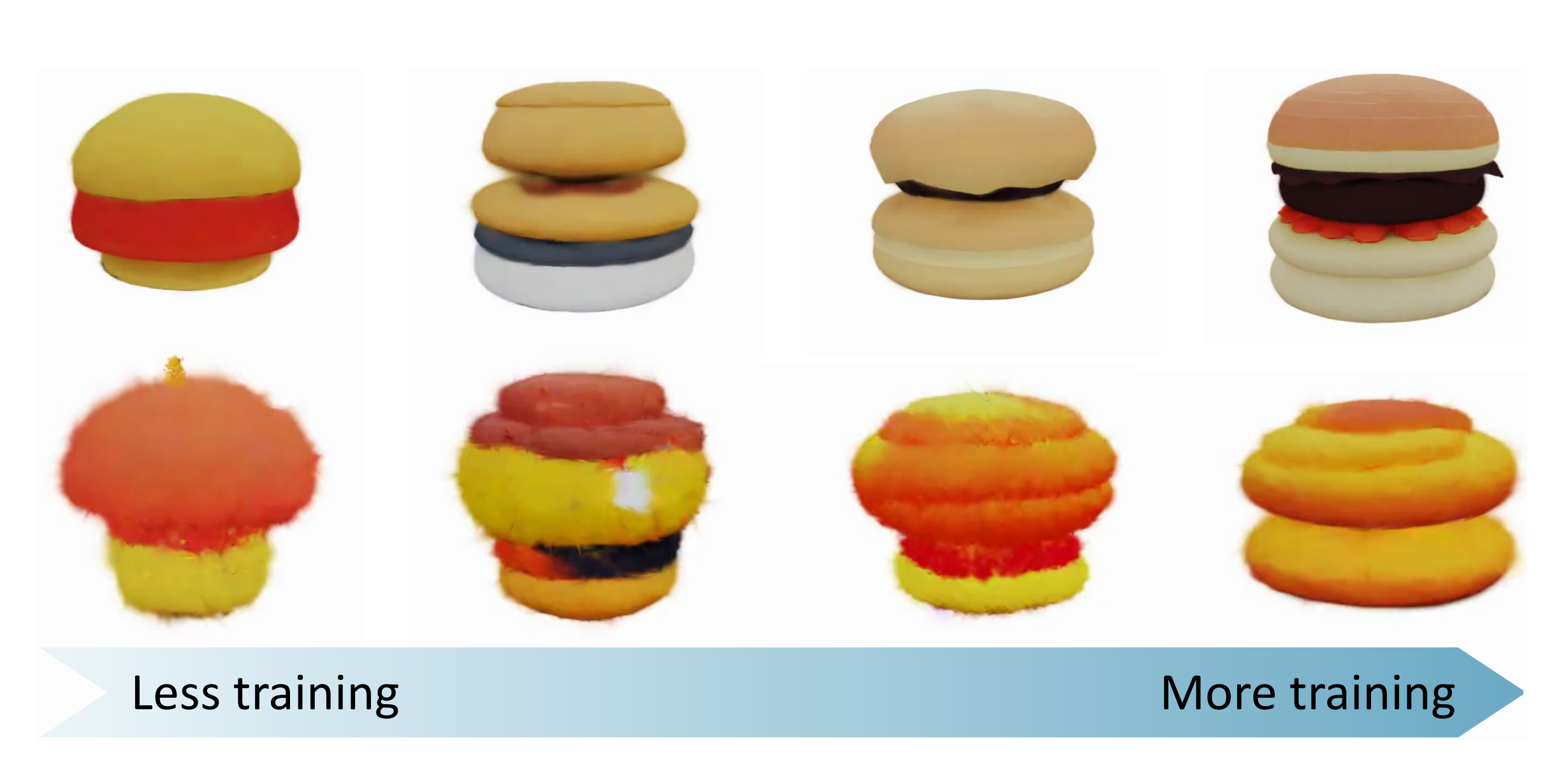
Pretraining improves both checkpoints in Figure 8: at 500K steps, CLIP/VQA rise from 19.33/0.23 when trained from scratch to 21.61/0.49; at one million steps they rise from 20.85/0.40 to 23.20/0.61. This supports faster learning and better final scores for this model/data setting, rather than universal transferability of any image diffusion model.
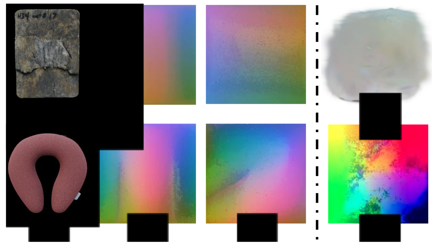
Replacing the shared transport construction with per-object neural flattening costs roughly another A100 GPU-year and yields less consistent atlas patterns and noisy generations at matched training steps in Figure 9. The evidence favors the proposed indexing over that tested alternative, not every possible learned parameterization.
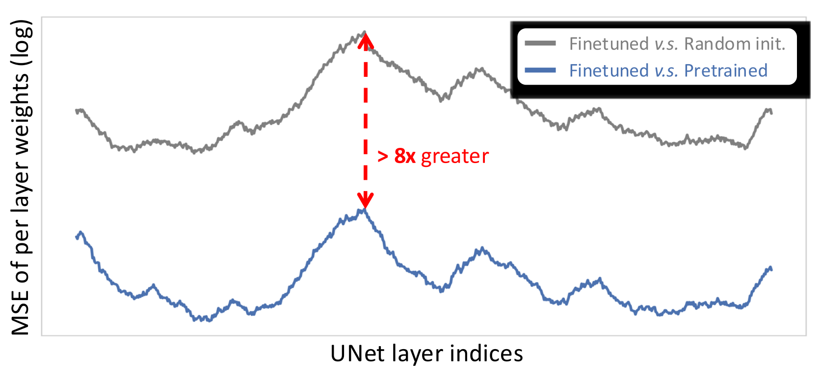
Figure 10 plots smoothed log mean-squared layer-weight differences. Fine-tuned weights remain much closer to pretrained weights than to random initialization, with more than an eightfold difference at the largest-change layer. Weight distance is descriptive evidence, not a causal proof of a better optimization basin or of general transfer.
7 Conclusion
Gaussian Atlas demonstrates a workable bridge from a pretrained image denoiser to Gaussian 3D generation. Its compact representation and reported alignment gains come with substantial fitted 3D training data and preprocessing. The evidence is strongest for the specific object-generation setup and initialization ablation tested here.
Acknowledgments.
The Stanford authors acknowledge NIH support, Panasonic, the Gordon and Betty Moore Foundation, the Jaswa family, Stanford HAI, a Stanford graduate fellowship, and the Wu Tsai Human Performance Alliance. They thank Fei Jiang and Moustafa Meshry for feedback.
Appendix A Supplementary for GaussianVerse
The supplement details Gaussian fitting, fit-quality comparisons, and the scale of related Gaussian datasets. Table 3 retains their published object and Gaussian counts.
| Methods | Venue | # of 3DGS fittings | # of Gaussians per fitting |
| GSD [30] | ECCV 2024 | 6,000 | 1,024 |
| GVGen [10] | ECCV 2024 | 46,000 | 32,768 |
| GaussianCube [57] | NeurIPS 2024 | 125,653 | 32,768 |
| ShapeSplat [27] | 3DV 2025 | 65,000 | 20,000 |
| GaussianVerse (ours) | - | 205,737 | 10,435 |
A.1 Fitting Details
Scaffold-GS uses four offsets per anchor to reduce duplicated Gaussians and permit more anchors initialized at random values. Fitting-loss weights are 0.8 for RGB, 0.2 for structural similarity, 0.02 for perceptual loss, and 0.01 for scale regularization. These are preprocessing weights, distinct from diffusion-training weights.
A.2 3DGS Quality of GaussianVerse
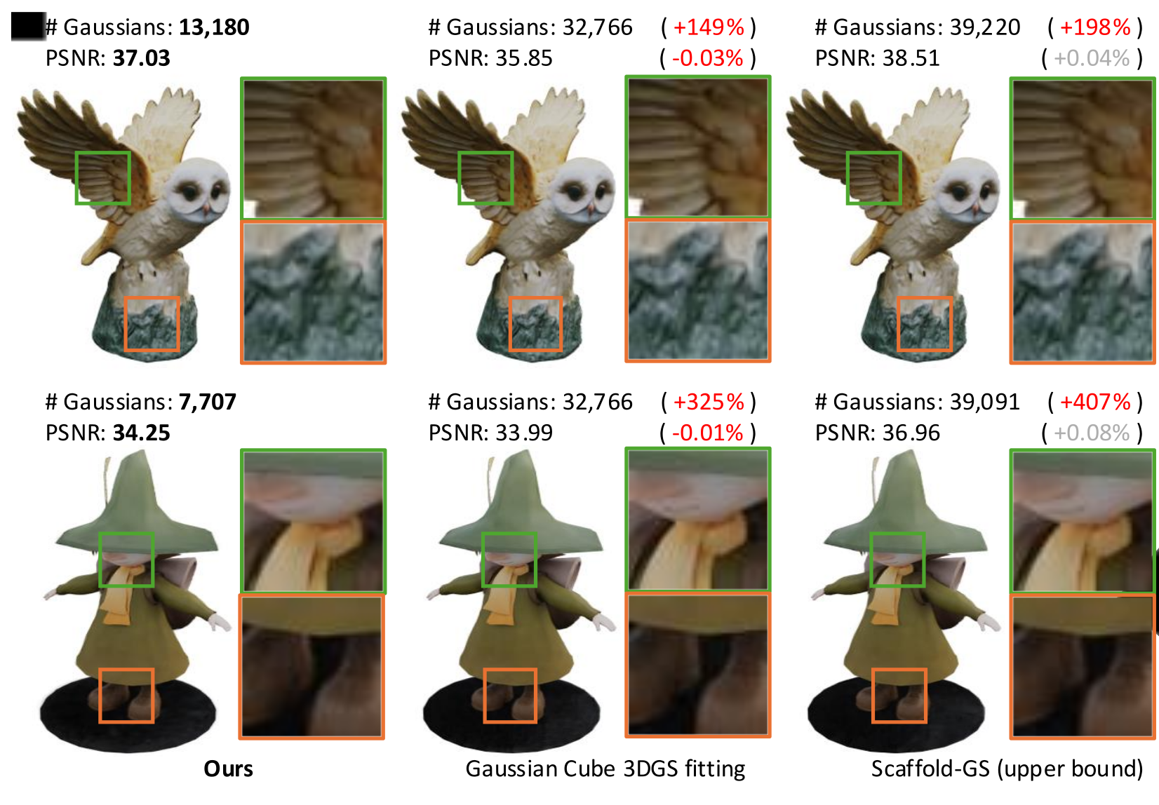
Figure 11 compares two example fits with GaussianCube’s constrained fitting and unconstrained Scaffold-GS. The proposed method uses 13,180 and 7,707 valid Gaussians while retaining comparable visible quality, versus roughly 32,766 and 39,000 primitives in the alternatives. Calling Scaffold-GS an upper bound refers to this comparison, not a formal optimality bound.
The figure’s PSNR percentage labels are inconsistent with its displayed values: for example, 37.03→35.85 is about −3.2%, not the printed −0.03%, and 34.25→36.96 is about +7.9%, not +0.08%. The original labels remain intact. These examples do not prove that all surplus Gaussians are redundant or that each fit has the minimum possible count.
A.3 Comparison with Other 3D Gaussian Datasets
Table 3 compares GaussianVerse’s 205,737 objects with GSD’s 6,000, GVGen’s approximately 46,000, GaussianCube’s 125,653, and ShapeSplat’s approximately 65,000. Unlike several fixed-count datasets, GaussianVerse varies the number of Gaussians per object. These are the datasets listed in the paper, not an exhaustive current inventory.
Appendix B Supplementary for Gaussian Atlas Formulation
The atlas supplement explains how variable-size fits become fixed-size training tensors while reusing the sphere-to-plane mapping.
B.1 Formulation Details
The initial transport can be nonsquare when the fitted object has fewer Gaussians than sphere points. Before final fixed-size assignment, smaller fits are padded by duplicating the smallest-scale Gaussians and setting the copies’ opacity to zero; larger fits lose the smallest-scale Gaussians. The target is 16,384 slots.
This padding preserves zero contribution from extra slots, while pruning can discard small geometric details. Constructing an atlas takes about one minute on average, an offline cost excluded from the reported generation latency.
Appendix C Supplementary for Finetuning LD with Gaussian Atlas
The diffusion supplement motivates removing the image autoencoder and specifies the training losses and memory settings.
C.1 Training Diffusion Model Without VAEs
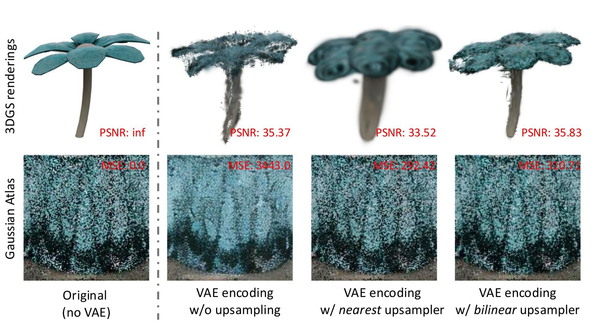
The pretrained image autoencoder is lossy and expects image-like RGB inputs at a much larger spatial resolution. Even upsampled atlases that appear similar in 2D can reconstruct Gaussian attributes inaccurately, changing the rendered object. Figure 12 retains the reconstruction errors and rendered views demonstrating this problem.
The original atlas has zero reconstruction error and infinite self-comparison PSNR; reconstructed versions have finite PSNR. Those values quantify this reconstruction experiment, not overall generation quality against ground-truth objects. Direct denoising avoids this autoencoder bottleneck while retaining the UNet’s pretrained weights.
C.2 More Details
Training combines attribute diffusion with photometric supervision on a randomly selected rendered view at every step.
Diffusion model training.
Loss weights are 1 for diffusion, 10 for RGB, 1 for mask, and 1 for perceptual similarity. Gradient checkpointing supports a local batch size of eight on each of eight GPUs, for total batch size 64. One sampled camera view supplies photometric losses per training step.
Appendix D More Results
Additional comparisons, prompt examples, and repeated-seed generations show the range and limitations of the learned model. All six supplementary generation figures are retained.
D.1 More Comparisons
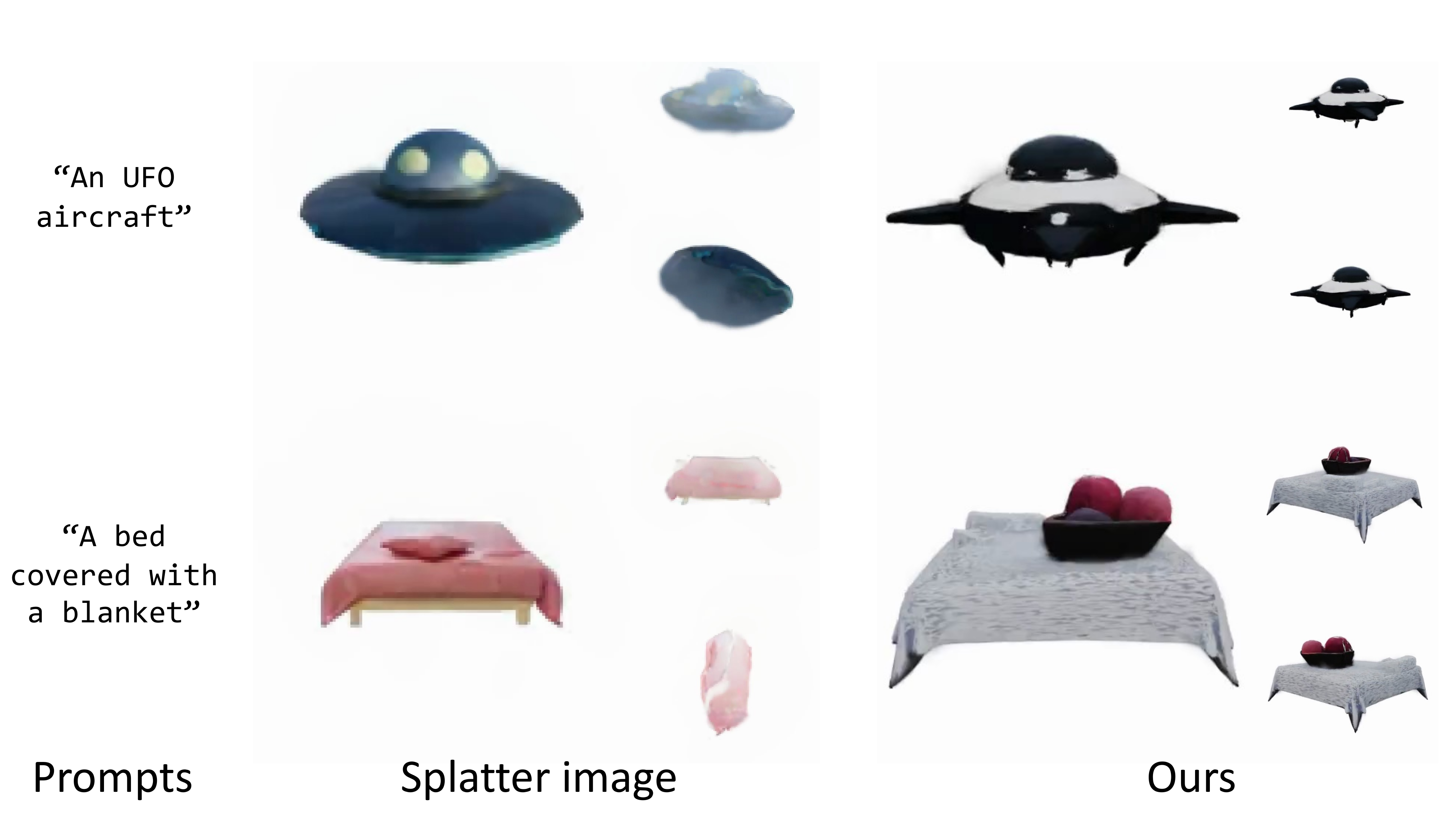
Figure 13 compares with Splatter Image initialized using MVDream-generated images. The selected examples show more detailed and coherent appearances for Gaussian Atlas. Splatter Image is an image-to-3D method in this setup; the comparison includes its generated-image initialization and does not isolate the reconstruction model from that input.
D.2 More Generations
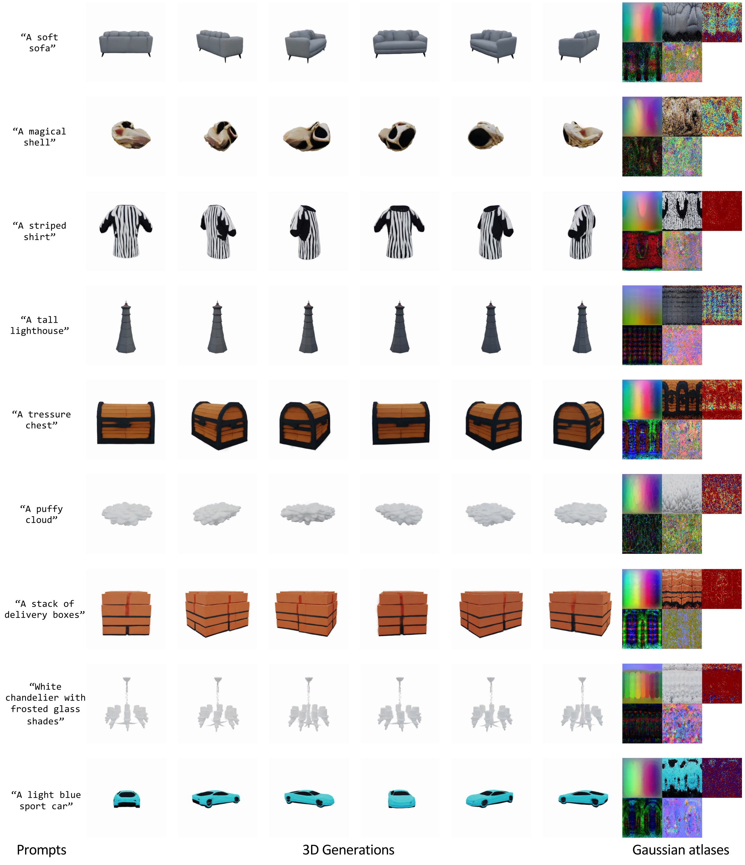
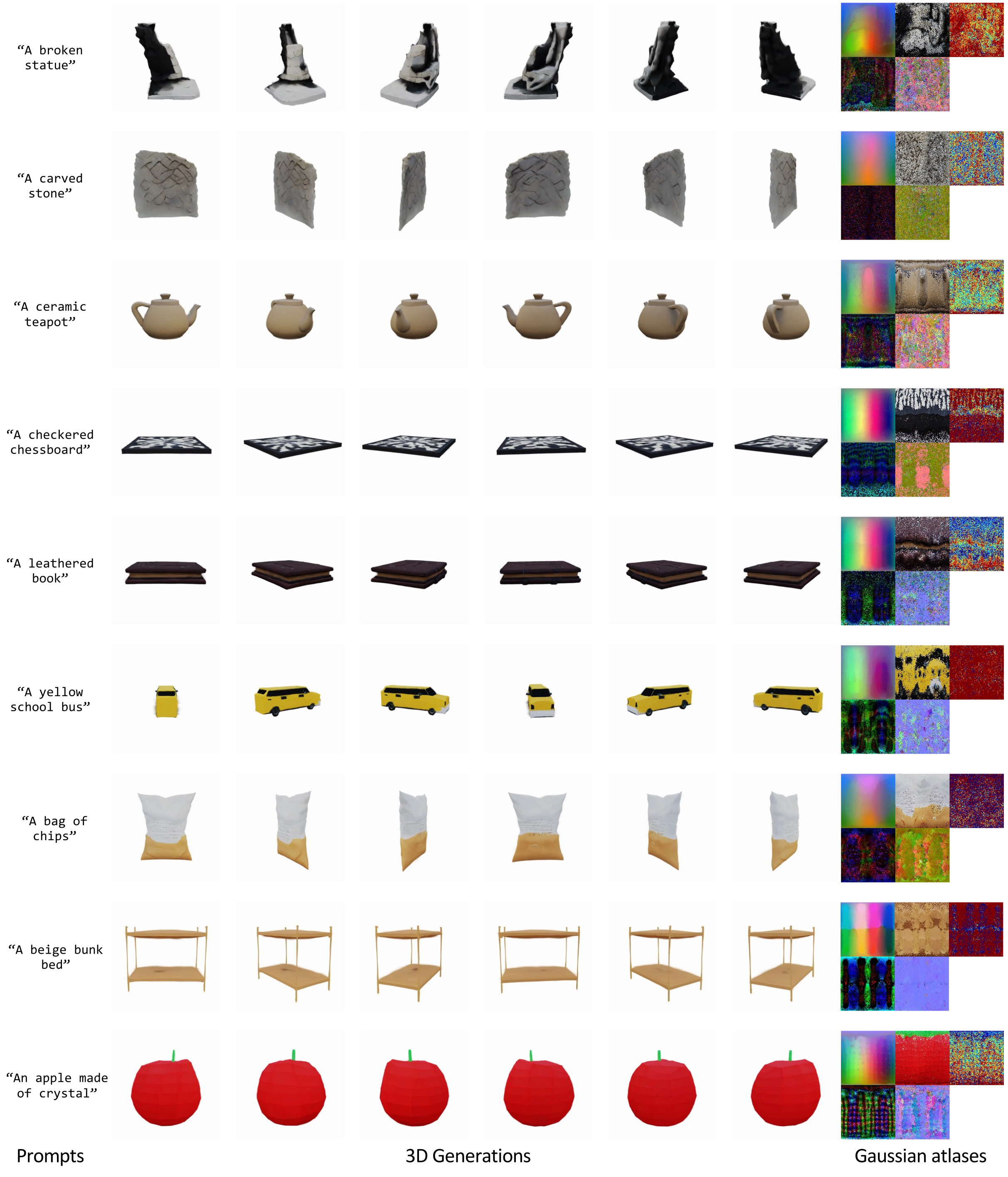
Figures 16 and 17 show objects prompted by color, shape, style, abstract properties, and quantity. The paper also refers to supplementary 360-degree videos. The displayed views show coherent objects without obvious atlas-seam artifacts in these examples, but do not establish a zero-artifact failure rate or accurate unseen geometry.
D.3 Diversity of Generations
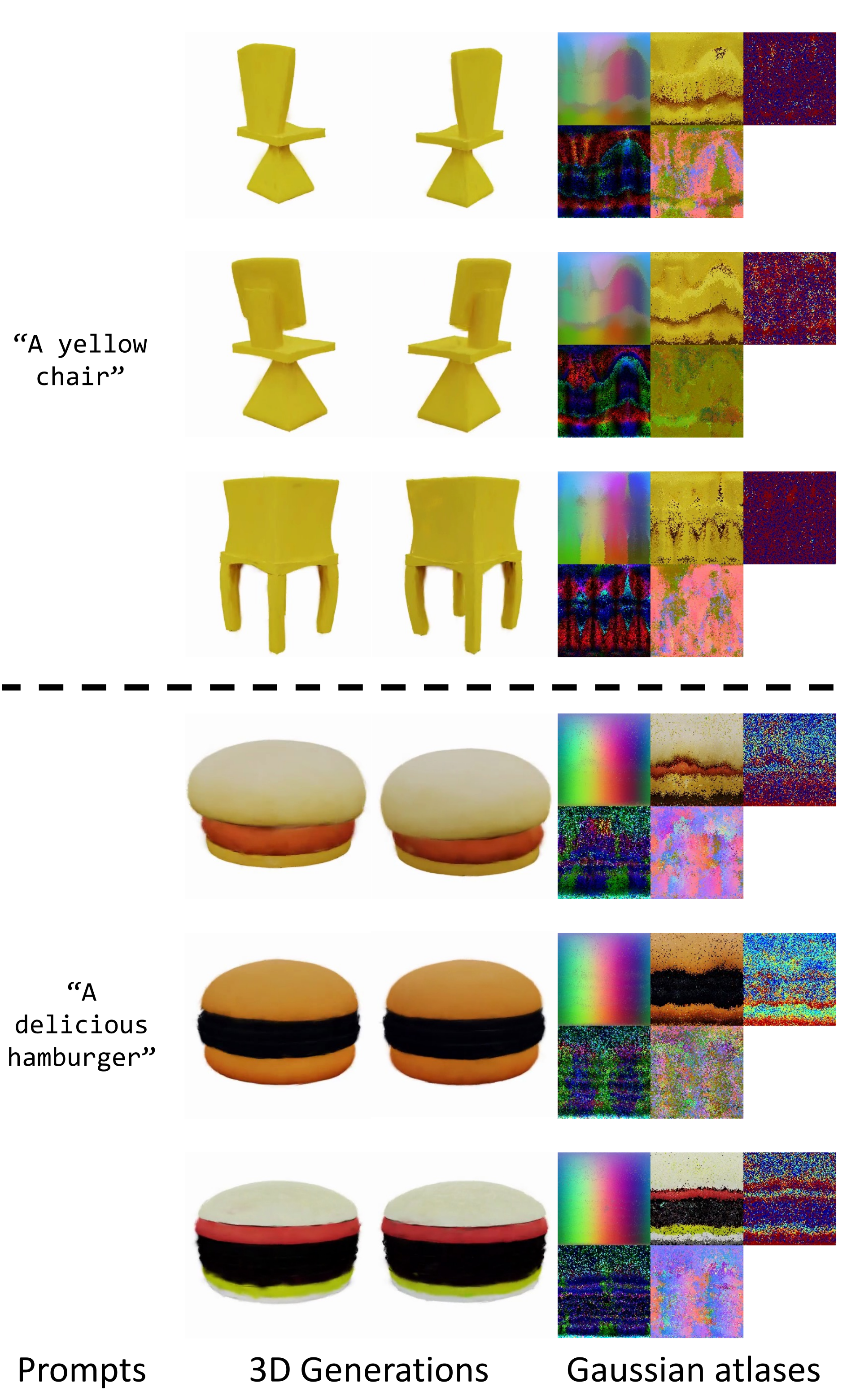
Figure 14 varies the initial diffusion noise under a fixed prompt, producing different chairs and hamburgers with their corresponding atlases. This demonstrates qualitative diversity; the paper does not quantify distribution coverage, repeated-sample fidelity, or whether every sample preserves all requested semantics.
Appendix E Discussions
The final discussion identifies representation capacity and inherited diffusion-model limitations, then outlines possible extensions.
Limitations.
Increasing the number of atlas slots improves potential detail but raises training and inference cost. The chosen 128×128 grid is a compromise, and output detail remains limited. The appendix’s claim of approximately three times fewer Gaussians than GaussianCube conflicts with Table 2’s 16K versus 33K; the reported counts indicate about half.
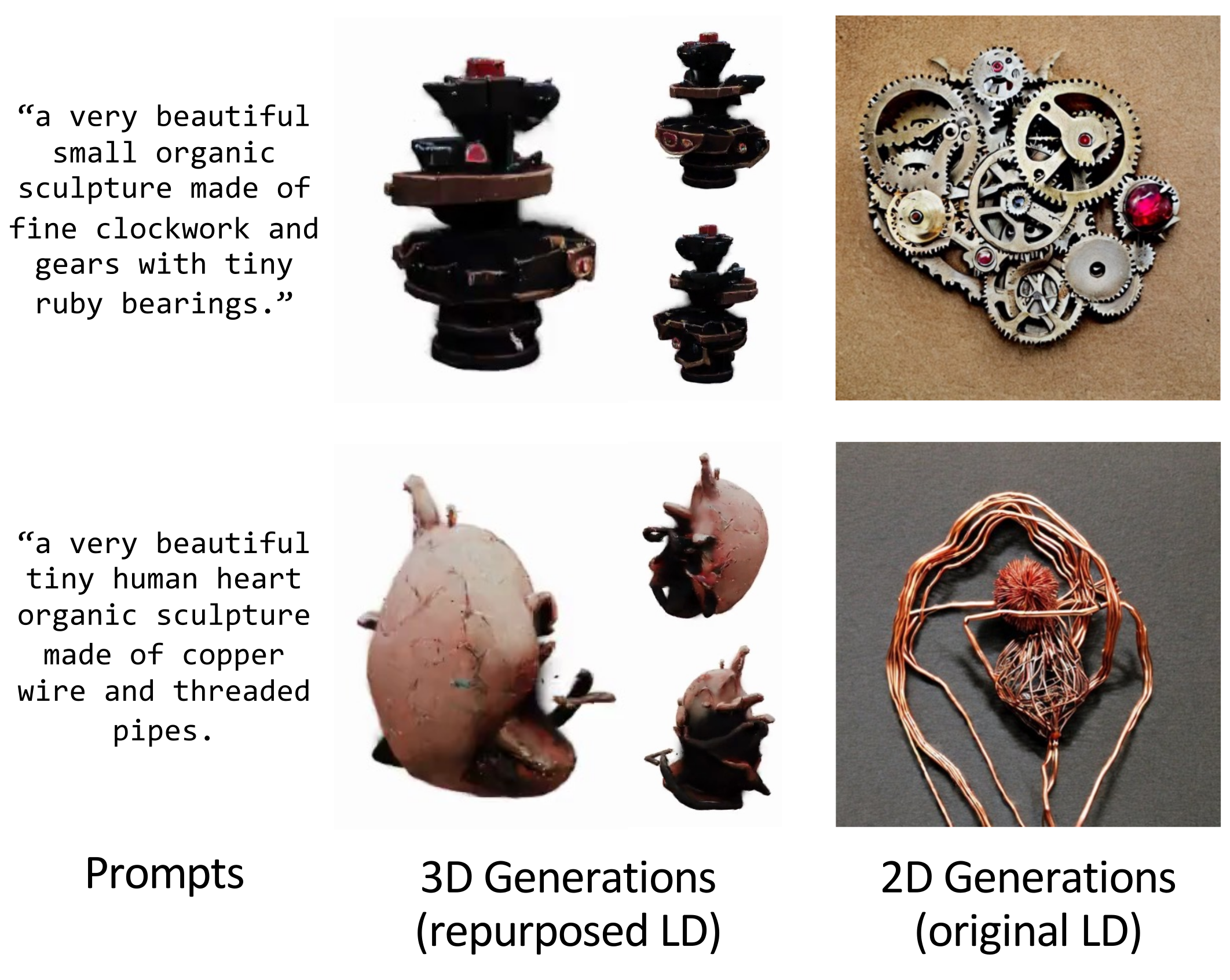
The model also inherits weaknesses of the selected latent diffusion checkpoint, notably long-prompt composition. Figure 15 retains two such failures alongside the original 2D model’s outputs. Success with shorter prompts does not imply reliable fine-grained attribute binding.
Future Directions.
Future directions include stronger diffusion backbones, transformer architectures, Gaussian latent diffusion, and adapting image-model extensions such as IP-Adapter and DreamBooth. These are proposed research directions, not capabilities implemented or evaluated in this paper.