Overview
The supplementary material includes all training settings, evaluation conventions, additional ablations, transfer and scaling experiments, wall-clock measurements, and four full-page reconstruction comparisons.
At a glance
FlowMo is a discrete image tokenizer with transformer encoders and a conditional rectified-flow decoder. Initial end-to-end training learns a distribution of plausible reconstructions; a second stage backpropagates perceptual loss through sampled reconstructions to favor modes resembling the source image. At two matched bit budgets on 256-pixel ImageNet reconstruction, it improves reconstruction FID, PSNR, and structural similarity over the selected baselines, though not LPIPS. Downstream generation shows mixed gains, and iterative decoding is substantially slower than a conventional tokenizer.
1 Introduction
Image tokenizers determine both reconstruction quality and the latent representation available to a later generative model. FlowMo replaces a conventional spatial latent grid and adversarial decoder training with a one-dimensional sequence of binary-quantized tokens and a conditional diffusion decoder.
The central idea is that accurately modeling every possible reconstruction is not the same as reconstructing a particular source image well. Perceptual post-training and a shifted sampling schedule deliberately concentrate the conditional distribution around useful modes. The claimed advantages apply to the tested compression budgets and metrics, rather than every measure of image fidelity or generation quality.
 |
 |
 |
 |
 |
 |
 |
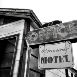 |
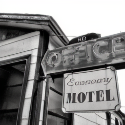 |
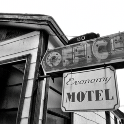 |
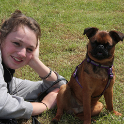
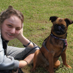
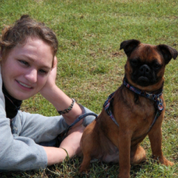
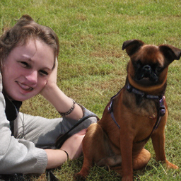
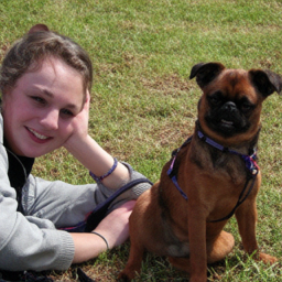
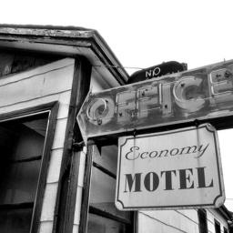
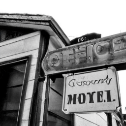
| Original image | OpenMagViT-V2 | FlowMo-Lo (Ours) | LlamaGen-32 | FlowMo-Hi (Ours) |
| (rFID=1.17) | (rFID=0.95) | (rFID=0.59) | (rFID=0.56) |
2 Related Work
The method builds on diffusion autoencoders [45], multimodal diffusion transformers [16], and perceptual optimization through diffusion sampling. Unlike approaches that distill a prior tokenizer or operate in its continuous latent space, FlowMo learns its pixel encoder and decoder directly.
Concurrent DiTo studies continuous diffusion tokenization, whereas FlowMo’s main experiments use discrete codes. A separate continuous variant is constructed specifically for that comparison. The learned perceptual losses remain important even though adversarial losses and an auxiliary tokenizer are absent.
3 Method
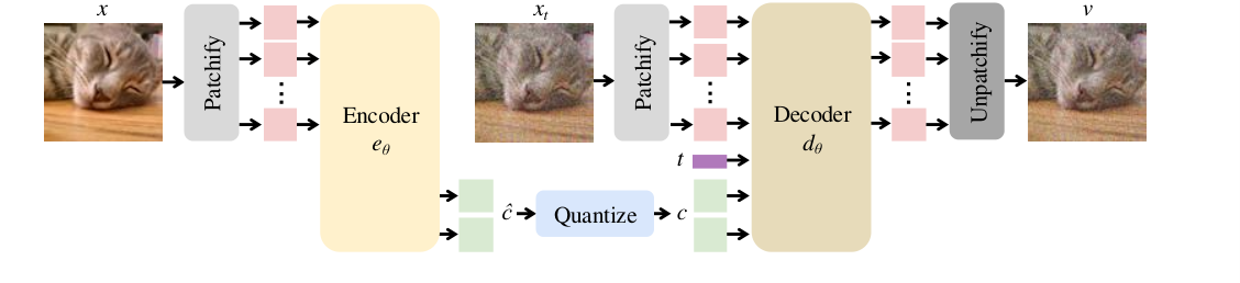
The tokenizer is trained in two phases: joint flow-based encoder–decoder training, followed by perceptual refinement with the encoder frozen. A separate masked-token generative model tests whether the resulting discrete representation is useful beyond reconstruction. Sampling choices are part of the reported reconstruction recipe.
3.1 Architecture
An MMDiT-style encoder jointly processes image patches and initially zero latent tokens through separate interacting streams. Lookup-free quantization maps each latent scalar to a binary value. A larger transformer decoder predicts a rectified-flow velocity from the noisy image, quantized code, and time embedding. The models use maximal-update parameterization to transfer hyperparameters across widths. The tokenizer architecture is transformer-based; its perceptual training networks are separate components.
Equations 1–3
| (1) |
| (2) |
| (3) |
3.2 Stage 1A: Mode-matching pre-training
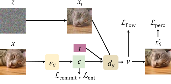
The first stage jointly trains encoder and decoder with velocity prediction across noise levels, a perceptual loss on the one-step denoised estimate, and lookup-free quantization entropy and commitment penalties. The perceptual network is LPIPS-VGG. Noise times follow a logit-normal mixture with ten percent uniform sampling, providing more coverage near the endpoints than a plain logit-normal schedule.
Equations 4–9
| (4) |
| (5) |
| (6) |
| (7) |
| (8) |
| (9) |
3.3 Stage 1B: Mode-seeking post-training
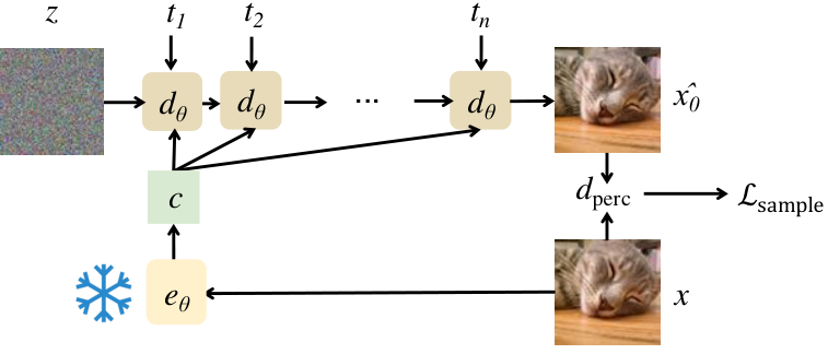
Freeze the encoder and optimize the decoder using both the flow objective and a perceptual loss on a complete generated reconstruction. Gradients pass through an eight-step sampling chain with randomly chosen times and checkpointing. A ResNet perceptual network replaces LPIPS-VGG for this stage, with sample-loss weight 0.01.
Small weights provide too little perceptual benefit; large weights can overfit the perceptual metric or destabilize training. Roughly one epoch and early stopping limit this behavior. Equation 12 and the method describe joint flow-plus-sample training, despite a later analysis sentence describing only the sample loss; the edition follows the explicit objective.
Equations 10–12
| (10) |
| (11) |
| (12) |
3.4 Sampling
At inference, reconstruction starts from Gaussian noise conditioned on the quantized code. A power-law timestep schedule with shift four concentrates steps at low noise while taking larger early steps. Together with limited-interval classifier-free guidance, this changes the reconstruction tradeoff. The default evaluation uses twenty-five decoding steps, so a token sequence does not decode in one forward pass.
Equations 13–14
| (13) |
| (14) |
3.5 Stage 2: Latent generative modeling
A MaskGiT [8] model learns the discrete code distribution. This second stage evaluates whether the tokenizer supports good generation under matched model-training resources, separately from how faithfully it reconstructs known input images.
4 Experiments
The experiments evaluate reconstruction at matched nominal bits per pixel, downstream generation, a continuous-tokenizer comparison, and architecture/training ablations. Reconstruction and generation FID use different reference distributions and should not be interchanged.
4.1 Main results
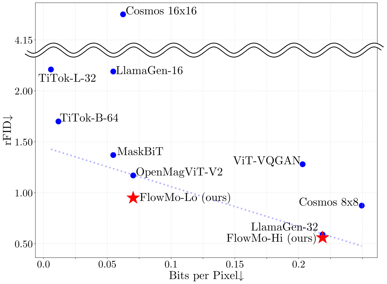
On 50,000 ImageNet validation images at 256×256, FlowMo-Lo uses about 0.0703 bits per pixel and improves reconstruction FID from OpenMagViT-V2’s 1.17 to 0.95, PSNR from 21.63 to 22.07, and SSIM from 0.640 to 0.649. LPIPS is slightly worse, 0.113 versus 0.111. At about 0.219 bits per pixel, FlowMo-Hi improves LlamaGen-32’s reconstruction FID from 0.59 to 0.56 and PSNR from 24.44 to 24.93, while LPIPS worsens from 0.064 to 0.073. The bit rate counts code capacity, not a demonstrated entropy-coded file size with overhead.
With matched MaskGiT training, FlowMo-Lo yields generation FID 4.30 versus 3.73 for OpenMagViT-V2, precision 0.86 versus 0.80, and recall 0.47 versus 0.51. Inception Score and spatial FID improve, but the overall generation result is mixed. Better reconstruction does not automatically make the latent distribution easier to model.
The separate continuous variant matches DiTo’s latent size and reports reconstruction FID 0.65 versus 0.78 and PSNR 26.61 versus 24.10. Main discrete models use eight H100s, 130 or eighty pretraining epochs, and approximately one post-training epoch. Smaller exploratory configurations supply the ablations. Model width, patch size, training length, and tokenizer type must be distinguished across these comparisons.
| Tokenizer | FID | IS | sFID | Prec. | Rec. |
| OpenMagViT-V2 | 3.73 | 241 | 10.66 | 0.80 | 0.51 |
| FlowMo-Lo (ours) | 4.30 | 274 | 10.31 | 0.86 | 0.47 |
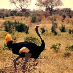
| Fully generated images - using OpenMagViT-V2 tokenizer (CFG=10.0) |
 |
 |
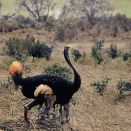
| Fully generated images - using FlowMo-Lo tokenizer (CFG=10.0) |
 |
 |
| Model | rFID | PSNR | SSIM | LPIPS |
| DiTo† [10] | 0.78 | 24.10 | 0.706 | 0.102 |
| FlowMo (ours) | 0.65 | 26.61 | 0.791 | 0.054 |
| BPP | Model | Tokens per image | Vocab size | rFID | PSNR | SSIM | LPIPS |
| 0.006 | TiTok-L-32 [61] | 32 | 2.21 | 15.60 | 0.359 | 0.322 | |
| 0.012 | TiTok-B-64 [61] | 64 | 1.70 | 16.80 | 0.407 | 0.252 | |
| 0.023 | TiTok-S-128 [61] | 128 | 1.71 | 17.52 | 0.437 | 0.210 | |
| 0.055 | LlamaGen-16 [51] | 256 | 2.19 | 20.67 | 0.589 | 0.132 | |
| MaskBiT† [55] | 256 | 1.37 | 21.5 | 0.56 | - | ||
| 0.062 | Cosmos DI-16x16 [61] | 256 | 4.40 | 19.98 | 0.536 | 0.153 | |
| 0.070 | OpenMagViT-V2 [38] | 256 | 1.17 | 21.63 | 0.640 | 0.111 | |
| FlowMo-Lo (ours) | 256 | 0.95 | 22.07 | 0.649 | 0.113 | ||
| 0.203 | ViT-VQGAN† [59] | 1024 | 1.28 | - | - | - | |
| 0.219 | LlamaGen-32 [51] | 1024 | 0.59 | 24.44 | 0.768 | 0.064 | |
| FlowMo-Hi (ours) | 1024 | 0.56 | 24.93 | 0.785 | 0.073 | ||
| 0.249 | Cosmos DI-8x8 [61] | 1024 | 0.87 | 24.82 | 0.763 | 0.072 |
4.2 Analysis
The smaller configuration’s ablations support fine image patches, end-to-end flow training, perceptual supervision, endpoint-aware time sampling, shifted decoding, and guidance. Removing perceptual supervision raises reconstruction FID from 2.87 to 13.86 even while PSNR improves, exposing the difference between pixel distortion and perceptual distribution quality. Finite scalar quantization also improves some pairwise metrics but worsens reconstruction FID relative to lookup-free quantization.
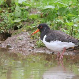
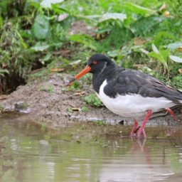
Post-training improves FlowMo-Lo from 1.10 to 0.95 reconstruction FID and FlowMo-Hi from 0.73 to 0.56, with PSNR and LPIPS also improving within each model. Repeated reconstructions remain stochastic, with more variance in backgrounds in the illustrated example. Tokenizer guidance drops the latent conditioning during training; it does not use class labels in the tokenizer.
 |
 |
| Original image | Reconstructed (discolored) |
| Model | rFID | PSNR | LPIPS |
| FlowMo (fewer params.) | 2.87 | 20.71 | 0.15 |
| with doubled patch size | 6.39 | 19.94 | 0.17 |
| with MSE-trained encoder | 3.82 | 21.40 | 0.15 |
| without perceptual loss | 13.86 | 22.11 | 0.21 |
| with FSQ quantization | 3.14 | 21.31 | 0.14 |
| with logit-normal schedule | 4.08 | 16.45 | 0.21 |
| without shifted sampler | 3.42 | 20.25 | 0.16 |
| without guidance | 3.28 | 20.67 | 0.16 |
| Model | rFID | PSNR | LPIPS |
| FlowMo-Lo | 1.10 | 21.38 | 0.134 |
| FlowMo-Lo (post-trained) | 0.95 | 22.07 | 0.113 |
| FlowMo-Hi | 0.73 | 24.02 | 0.086 |
| FlowMo-Hi (post-trained) | 0.56 | 24.93 | 0.073 |
 |
 |
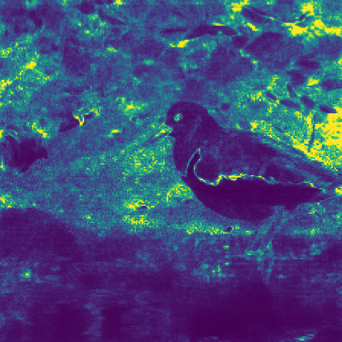 |
| Original image | Reconstructed | Variance heatmap |
Limitations.
The main limitation is iterative inference: twenty-five decoding steps require many model evaluations, and backpropagation through sampling also makes post-training expensive. The model may overfit its perceptual objective, prompting early stopping. Later timing measurements quantify the decoding cost; proposed distillation speedups are not demonstrated here.
5 Conclusion
FlowMo shows that a directly trained transformer diffusion autoencoder can be competitive for discrete perceptual image reconstruction at the tested bit budgets. Its strongest evidence is reconstruction quality; LPIPS, downstream generation, and decoding speed expose tradeoffs. The work acknowledges ONR MURI support.
Appendix A Training setup and hyperparameters
The supplementary setup records optimizer settings, losses, architecture sizes, token factorization, and separate recipes for tokenizer pretraining, post-training, and latent generation.
A.1 Stage 1A - Tokenizer pre-training
Lookup-free quantization uses relatively low commitment weight, and token factorization makes the entropy calculation manageable. Hyperparameters are selected on a smaller model and transferred to the larger configurations. Table 6 lists a 517-million-parameter exploratory model and 945-million-parameter main models, with four-pixel patches for the latter.
The high-rate representation is listed as 256 tokens of 56 bits in the architecture table and 1,024 tokens of fourteen bits in the benchmark table; both total 14,336 bits, consistent with code factorization. The main prose says only decoder width increases, whereas Table 6 gives a single hidden-width value, so the table does not independently resolve encoder width. All original settings are retained.
| Hyperparameter | FlowMo (fewer params) | FlowMo-Lo | FlowMo-Hi |
| Learning rate | 0.0001 | - | - |
| Batch size | 128 | - | - |
| Weight decay | 0 | - | - |
| Num. epochs | 40 | 130 | 80 |
| 0.0025 | - | - | |
| 0.000625 | - | - | |
| 0.1 | - | - | |
| Hidden size ( width) | 768 | 1152 | 1152 |
| MLP ratio | 4 | - | - |
| Encoder patch size | 8 | 4 | 4 |
| Decoder patch size | 8 | 4 | 4 |
| Encoder depth | 8 | - | - |
| Decoder depth | 16 | - | - |
| Latent sequence length | 256 | - | - |
| Latent token size | 18 | 18 | 56 |
| Codebook size for entropy loss | 9 | 9 | 14 |
| Total number of parameters | 517 | 945 | 945 |
A.2 Stage 1B - Tokenizer post-training
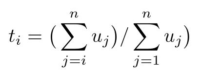
Replacing the one-step perceptual loss with a ResNet network does not match full-chain post-training in the loss-weight sweep: reconstruction FID is 1.28 for the sampled-chain loss versus a best listed 1.60 for the one-step alternatives. Post-training uses batch size 64, learning rate 0.00005, gradient accumulation and checkpointing, and about one epoch. The retained timestep equation normalizes cumulative random draws to set the sampled integration times.
| Loss type | Loss weight | rFID |
| 0.01 | 1.28 | |
| 0.05 | 2.57 | |
| 0.01 | 2.38 | |
| 0.005 | 2.16 | |
| 0.001 | 1.67 | |
| 0.0005 | 1.61 | |
| 0.0001 | 1.81 | |
| 0.00025 | 1.64 | |
| 0.0005 | 1.61 | |
| 0.00075 | 1.60 |
Equation
 |
A.3 Stage 2 - Generative model training
The second-stage transformer has hidden size 1,024, twenty-eight layers, and 397 million parameters. Both tokenizers supply 256 eighteen-bit codes, split into 512 nine-bit tokens for masked-token training. Models train for 300 epochs at batch size 128 and learning rate 0.0001. Sampling uses 64 steps and separately tuned temperatures. The stated generative guidance is 1.5, while Figure 6’s qualitative grid labels CFG 10.0; the figure should not be assumed to show the exact quantitative evaluation setting.
Appendix B Evaluation setup and hyperparameters
Tokenizer evaluation uses guidance weight 1.5 within rectified-flow noise levels approximately 0.145–0.505. Reconstruction metrics compare the full 50,000-image validation set with its reconstructions. Generation uses 50,000 samples and training-set reference statistics. These conventions differ from the five-thousand-sample tradeoff experiment and from the perceptual post-training loss itself.
Appendix C Additional Experiments
Additional experiments examine perceptual tradeoffs, new datasets and resolutions, scaling, precision and recall, other model variants, and measured encoding/decoding times.
C.1 Rate-distortion-perception tradeoff
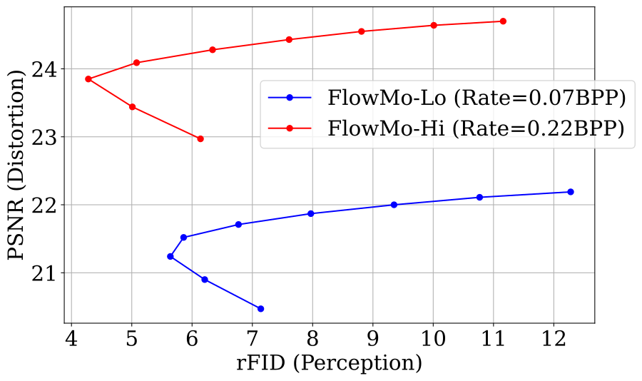
Changing the norm of the initial Gaussian noise traces a tradeoff between reconstruction FID and PSNR, rather than reproducing the simultaneous gains of the proposed recipe. Increasing apparent source-noise likelihood is not the same as maximizing full image likelihood, which also depends on the flow Jacobian. Figure 9 uses 5,000 samples per setting; the experiment does not evade general rate–distortion–perception tradeoffs.
C.2 Dataset and resolution generalization.
Patchwise diffusion and blending extend evaluation from 256 to 512 resolution and to OpenImages and Food-101. Table 8 labels the evaluated model FlowMo-Hi, despite the surrounding prose naming FlowMo-Lo. It improves reconstruction FID over Cosmos DI-8×8 on five of six listed dataset/resolution combinations, but is worse on Food-101 at 256 resolution, 1.39 versus 1.05. These are limited transfer tests rather than universal resolution-independent superiority.
| ImageNet-1K | OpenImages | Food-101 | ||||
| Resolution | 256 | 512 | 256 | 512 | 256 | 512 |
| Cosmos DI-8x8 | 0.87 | 0.39 | 0.85 | 0.52 | 1.05 | 0.94 |
| FlowMo-Hi | 0.55 | 0.30 | 0.69 | 0.40 | 1.39 | 0.68 |
C.3 Tokenizer scaling.
At a fixed 200,000 training steps, increasing width raises model size from 260 to 710 million parameters and improves reconstruction FID from 7.77 to 3.84, PSNR from 20.84 to 21.70, and LPIPS from 0.169 to 0.152. The comparison holds steps fixed, so larger models also use more computation; it is not a fixed-FLOP scaling result.
C.4 “Mode-seeking,” precision and recall
When reconstructions and references correspond image by image, post-training improves both measured precision and recall. Against separate training-set statistics, precision rises from 0.734 to 0.766 while recall falls from 0.660 to 0.634. This supports the interpretation that the decoder favors higher-fidelity modes while reducing some distributional diversity, rather than proving diversity is always preserved.
| vs. train stats. | vs. val stats. | |||
| Model name | Prec. | Rec. | Prec. | Rec. |
| FlowMo (fewer params) (no posttrain) | 0.734 | 0.660 | 0.974 | 0.988 |
| FlowMo (fewer params) | 0.766 | 0.634 | 0.993 | 0.991 |
C.5 More results with post-training
Additional post-training examples improve the smaller discrete model from 2.02 to 1.21 reconstruction FID and the continuous variant from 0.74 to 0.65, with accompanying PSNR and LPIPS gains. These configuration-specific numbers supplement the main models and should not be substituted for the earlier differently trained ablation baseline.
C.6 Wall clock times
The timing table reports 0.050 seconds to encode and 2.391 seconds to decode an image for the model labeled FlowMo-B, versus 0.021 and 0.038 seconds for LlamaGen-32. The listed small model takes 0.011 and 0.322 seconds. The full diffusion decoder is therefore about 63 times slower in that table, while encoding is much closer. The local table does not identify a complete timing hardware/batch protocol; the suggested five-to-tenfold distillation speedup is future work.
| Model name | Encode 1 image (s) | Decode 1 image (s) |
| LlamaGen-32 | 0.021 | 0.038 |
| FlowMo-B | 0.050 | 2.391 |
| FlowMo-B (small) | 0.011 | 0.322 |
Appendix D Extended visualization
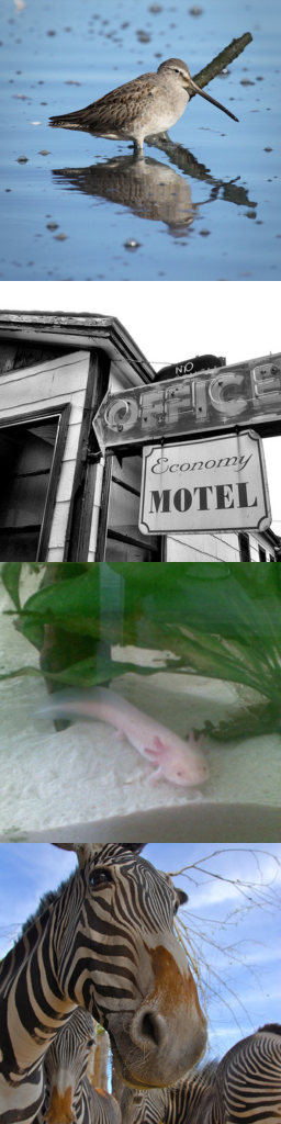
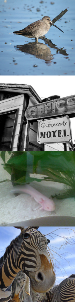
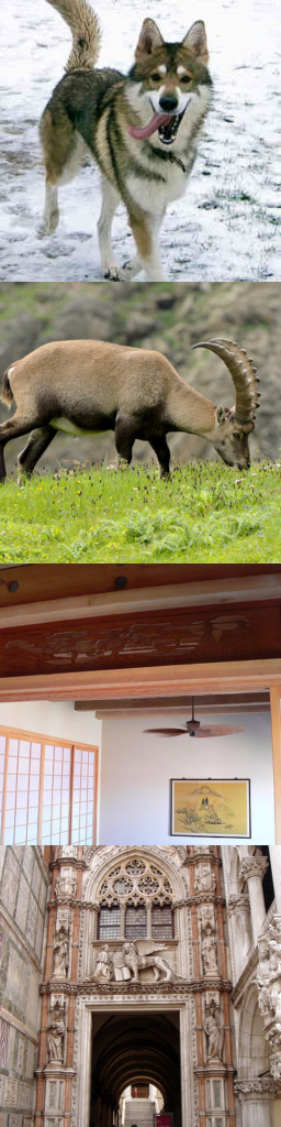
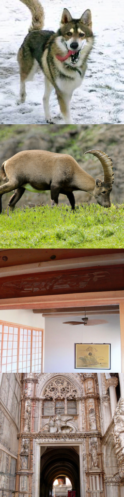
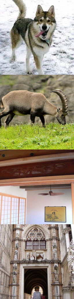
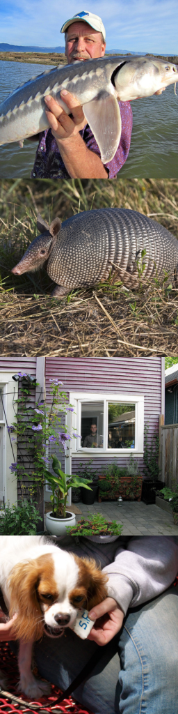
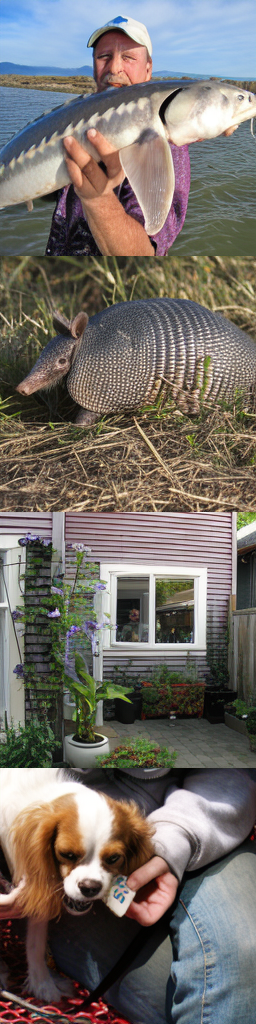
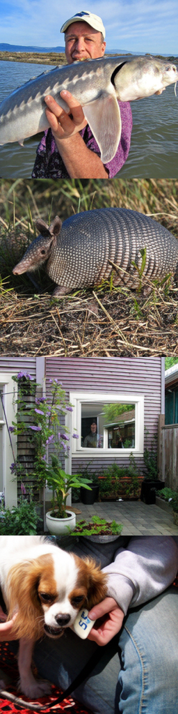
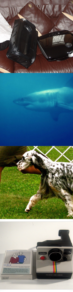
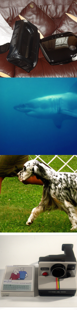
Four full-page grids compare original images with low-rate OpenMagViT-V2/FlowMo and high-rate LlamaGen/FlowMo reconstructions. Every image and column is retained at original resolution, including text, faces, animals, transparent objects, and fine textures. The authors state these examples were not cherry-picked; they illustrate local differences alongside the aggregate metrics.
 |
 |
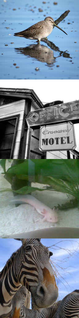 |
| Original image | Reconstructed | Reconstructed |
| (OpenMagViT-V2 [38]) | (FlowMo-A) |
 |
 |
 |
| Original image | Reconstructed | Reconstructed |
| (OpenMagViT-V2 [38]) | (FlowMo-A) |
 |
 |
 |
| Original image | Reconstructed | Reconstructed |
| (LlamaGen-32 [51]) | (FlowMo-B) |
 |
 |
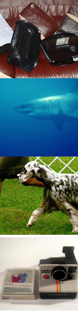 |
| Original image | Reconstructed | Reconstructed |
| (LlamaGen-32 [51]) | (FlowMo-B) |