At a glance
TrajHF adapts a diffusion driving planner to two annotated styles, aggressive and defensive. It learns a reward from human preferred trajectories paired with normalized model-generated alternatives, then updates the denoising policy using group-relative rewards, a frozen-policy behavior-cloning regularizer, and a final supervised refresh. On selected internal clips, professional annotators rate the resulting trajectories better or equal to the pretrained policy more often than those from supervised fine-tuning. NavSim evaluates the base planning architecture separately with a benchmark-score reward. These results support style adaptation in the tested data, but do not establish individual-driver personalization or closed-loop safety of the preference-tuned policies.
1 Introduction
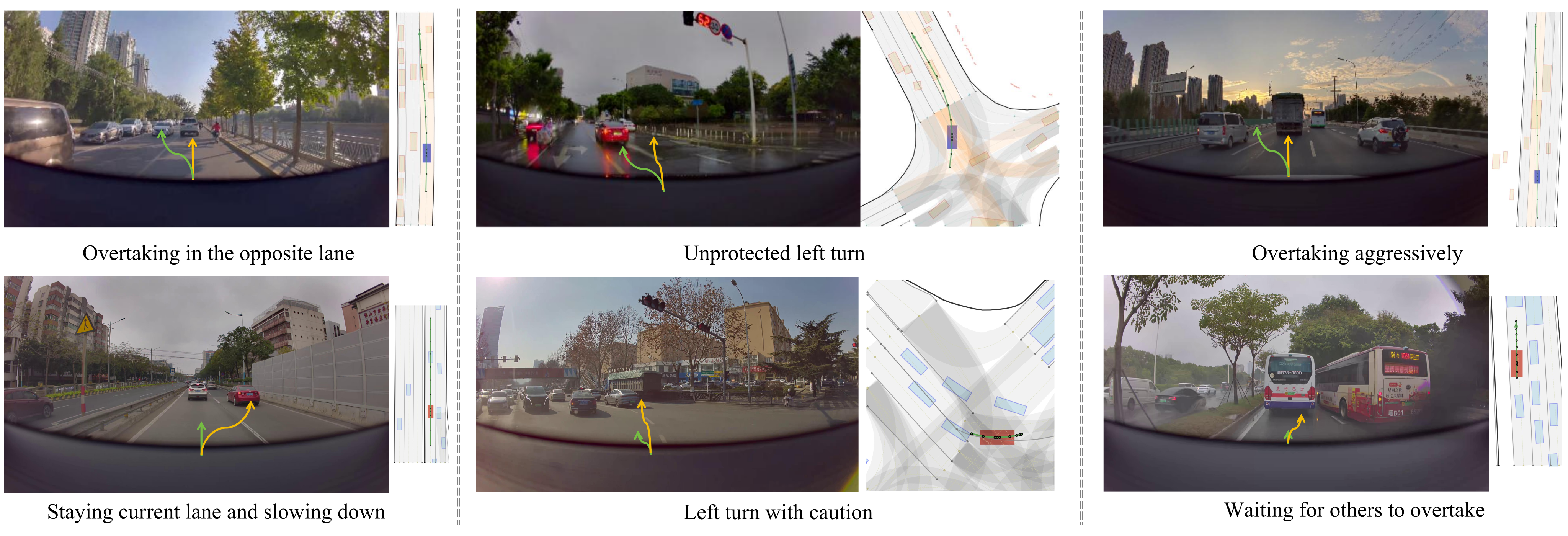
Demonstration learning can underrepresent rare driving preferences even when it models multiple plausible trajectories. Examples in Figure 1 contrast proceeding assertively, overtaking, and borrowing an opposing lane with waiting, slowing, or yielding. TrajHF treats these styles as preferences that can be learned from selected human takeover behavior. Its two contributions are a multimodal-conditioned diffusion planner and a reward-guided adaptation procedure.
The target is an annotated style distribution, not a single universally preferable maneuver. Aggressiveness, speed, safety, and contextual appropriateness are separate properties. The paper’s preference data and qualitative examples do not by themselves verify that every style-consistent trajectory is safe or lawful in closed-loop interaction.
2 Related Work
The method builds on continuous trajectory generation and preference optimization, using shared perceptual conditioning for both the planner and its learned reward model.
2.1 End-to-end Trajectory Planning
Imitation planners range from direct regression to discrete trajectory vocabularies. UniAD, ViP3D, VAD, and Hydra-MDP structure perception and planning in different ways; Transfuser [14] fuses camera and LiDAR features. TrajHF generates continuous trajectories from noise and avoids predefined anchors or trajectory vocabularies. This architectural distinction is evaluated on NavSim [8].
2.2 Generative Trajectory Models
GANs, VAEs, autoregressive models, and diffusion models all represent multimodal motion. DiffusionDrive and GoalFlow improve inference or condition trajectories on goals. TrajHF adds style-focused reward adaptation to a diffusion planner; it does not show that generic generative models intrinsically cannot represent the same styles with sufficient data.
2.3 Finetuning with Human Feedback
RLHF [23] learns from preference information rather than solely matching demonstrations. Related diffusion and driving methods use reward models, direct preference optimization, or KL regularization. TrajHF adopts critic-free group-relative advantages inspired by GRPO [31] and a reference-policy cloning term, with comparisons to a reimplemented PPO method and DPO in Appendix C.
3 Problem Definition
A trajectory is a sequence of ego states. Equations 1–3 describe imitation learning as matching an aggregate data distribution that mixes latent style distributions. Equation 4 introduces a reward-maximizing preference distribution as a conceptual target. The implemented procedure does not estimate the mixture weights or prove recovery of each driver’s latent distribution; it trains separate style-oriented models from chosen trajectories and contextual observations.
Equations 1–4
| (1) |
| (2) |
| (3) |
| (4) |
4 Method
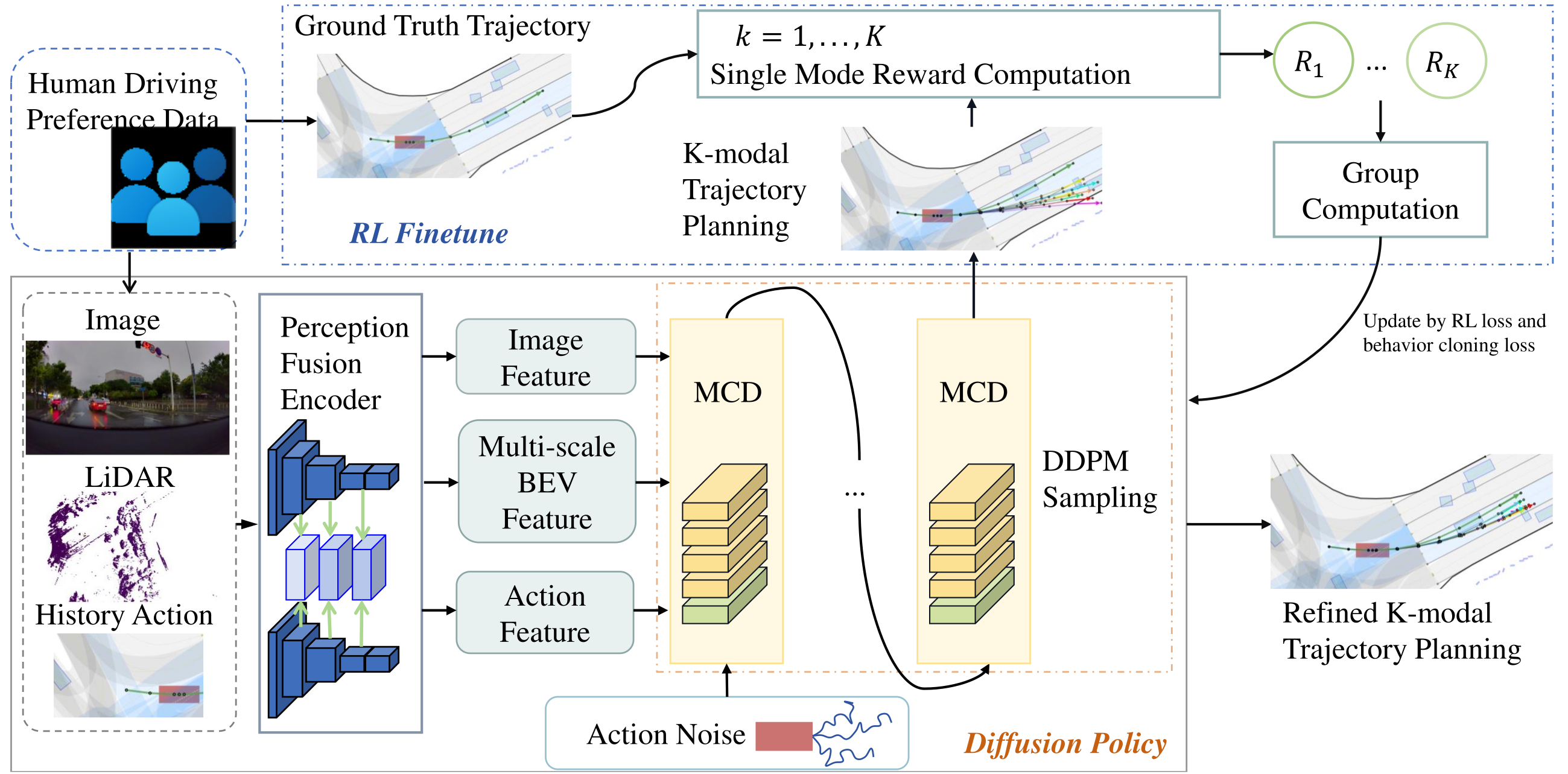
The system first learns a multimodal denoising planner, then uses a learned trajectory reward to reshape its output distribution. Figure 2 and Algorithm 1 preserve the full training and inference structure.
4.1 Generative Trajectory Model
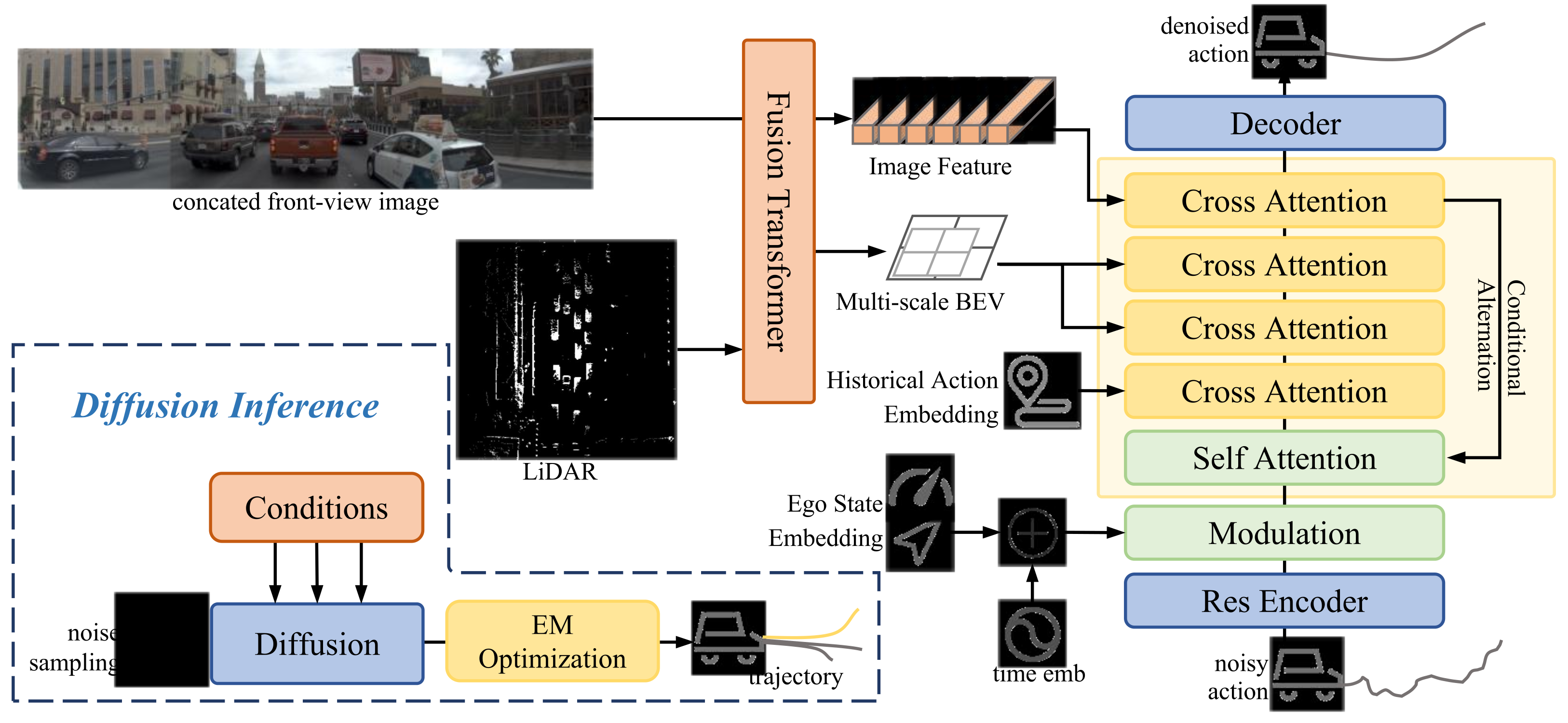
DDPM training predicts Gaussian noise at a sampled noise level, conditioned on front-view imagery, LiDAR, past actions, and ego state. Equations 5–6 retain the reverse diffusion update and denoising objective. Before adding noise, state trajectories are converted to successive state differences, reducing variation in scale over the horizon; accumulating these increments recovers the trajectory.
The multi-conditional denoiser uses a residual MLP action encoder, time/ego-state modulation, and repeated cross-attention to image, BEV, and historical-action features. Camera and LiDAR backbones exchange information through fusion transformers; intermediate fused maps provide a higher-resolution BEV condition. Figure 3 preserves all these branches. At inference, multiple noise samples produce candidate trajectories, followed by an EM-like representative-trajectory calculation. This selection favors the sampled distribution’s coverage, rather than explicitly maximizing a verified safety objective.
Equations 5–6
| (5) |
| (6) |
4.2 Driving Preferences Alignment
The preference dataset pairs each observation with a chosen human trajectory. Normal trajectories sampled from the pretrained planner provide rejected alternatives after an autoencoder reduces easy distributional cues. A reward model reuses the denoiser’s perceptual architecture and maps the trajectory representation to a scalar. Equation 7 combines Bradley–Terry ranking loss [35] with a margin penalty, encouraging the chosen trajectory to score above its synthetic alternative. Human annotation supplies the chosen style behavior; each synthetic pair is not independently ranked by a human.
DPGRPO treats the reverse denoising chain as a finite-horizon stochastic policy. For one observation/noise condition it generates K trajectories, evaluates only their terminal outputs, and normalizes the group’s rewards by their mean and standard deviation (Equation 8). Equation 9 weights denoising-step log probabilities by discounted group-relative advantages. The displayed objective is a REINFORCE-style update; no PPO clipping ratio is included in it. The paper does not specify handling of an exactly zero group reward variance.
A frozen pretrained model supplies reference denoising rollouts. Equation 10 encourages the updated policy to retain likelihood on those rollouts, and Equation 11 weights this cloning penalty against the reward objective. After RL converges, supervised training on preferred demonstrations reduces residual drift. Consequently, the reported RL pipeline includes this final supervised refresh; its contribution is not isolated by a separate ablation. Equation 9’s 1…T index differs from the appendix’s 0…T−1 convention, an implementation detail that must be reconciled rather than copied literally.
Equation 7
| (7) |
Input: diffusion policy ,
dataset of the target driving style ,
group size .
Output: finetuned policy .
Equations 8–11
| (8) |
| (9) |
| (10) |
| (11) |
5 Experiments
Experiments separate general planning on NavSim from style adaptation on proprietary normal/preference data. The main tables, all appendix ablations, and all qualitative panels are preserved.
5.1 Experimental Setup
NavSim uses PDMS and its collision, drivable-area, progress, time-to-collision, and comfort components. Internal datasets use minimum and mean average/final displacement errors across generated candidates, plus diversity. Minimum errors describe whether at least one candidate matches the recorded trajectory; they do not measure the quality of whichever candidate a deployed controller selects. Better or Equal Rate (BOE) adds a subjective style comparison against the pretrained policy and counts ties as success.
5.2 Main Results
The two evaluations answer different questions: NavSim measures general benchmark planning after score-based refinement, while internal tests measure style matching and retention of normal driving behavior after preference adaptation.
5.2.1 NavSim Benchmark
All listed NavSim methods use cameras and LiDAR, and TrajHF is trained only on the NavSim trainval split for this comparison. Fine-tuning uses PDMS itself as reward, rather than the human-style reward model. A single sample scores 86.4 PDMS; EM selection from 15 samples improves this to 87.6, above Hydra-MDP’s 86.5 but below DiffusionDrive’s 88.1 and GoalFlow’s 90.3. Choosing a candidate with the PDMS oracle reaches 94.3; the table explicitly treats this as an upper bound, not the ordinary EM selector’s performance. The results show useful candidate coverage, not state-of-the-art deployed selection or preference-tuned closed-loop safety.
| Method | Paradigm | |||||||
|---|---|---|---|---|---|---|---|---|
| Transfuser (Chitta et al., 2022) | AR | 97.8 | 92.6 | 78.9 | 92.9 | 100 | 83.9 | |
| Hydra-MDP (Li et al., 2024) | AR | 98.3 | 96.0 | 78.7 | 94.6 | 100 | 86.5 | |
| DiffusionDrive (Liao et al., 2024b) | Diffusion | 98.2 | 96.2 | 82.2 | 94.7 | 100 | 88.1 | |
| GoalFlow (Xing et al., 2025) | Diffusion | 98.4 | 98.3 | 85.0 | 94.6 | 100 | 90.3 | |
| TrajHF (Single sample) | Diffusion | 96.3 | 96.0 | 83.1 | 91.5 | 100 | 86.4 | |
| TrajHF (EM) | Diffusion | 96.6 | 96.6 | 84.5 | 92.1 | 100 | 87.6 | |
| TrajHF (PDMS selector) | Diffusion | 99.2 | 99.1 | 90.2 | 97.7 | 100 | 94.3 |
5.2.2 Human Preference Finetuning
On aggressive clips, RL yields minADE/minFDE 0.5304/1.2788 versus supervised fine-tuning’s 0.5416/1.3147; BOE against pretraining is 0.7660 versus 0.6577. Defensive results are 0.3101/0.8092 versus 0.3175/0.8351, with BOE 0.7922 versus 0.7430. Each BOE compares with the pretrained model separately, so these are not direct RL-versus-SL win rates. The mean errors sometimes favor SL, and the defensive mean errors exceed pretraining despite better minimum errors.
Retention on normal data is better for RL than SL in most error metrics, but both degrade substantially from pretraining. For aggressive RL, normal minADE rises from 0.2330 to 0.3777 and meanFDE from 2.1207 to 3.8057. For defensive RL, these become 0.3361 and 7.4631. Thus the source’s claim of no significant performance degradation is not supported relative to the pretrained baseline; the favorable comparison is mostly against supervised adaptation. No statistical significance test is provided.
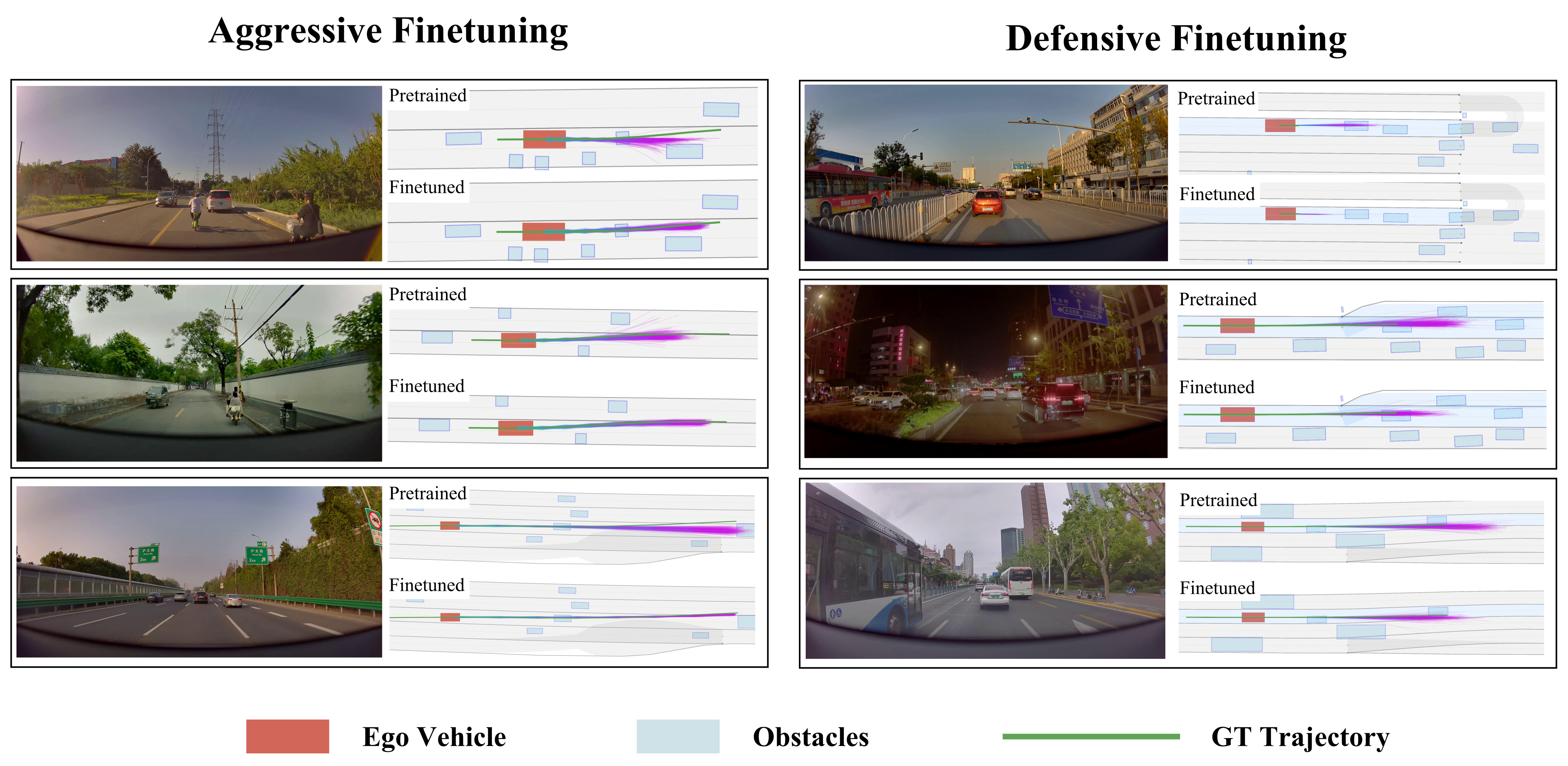
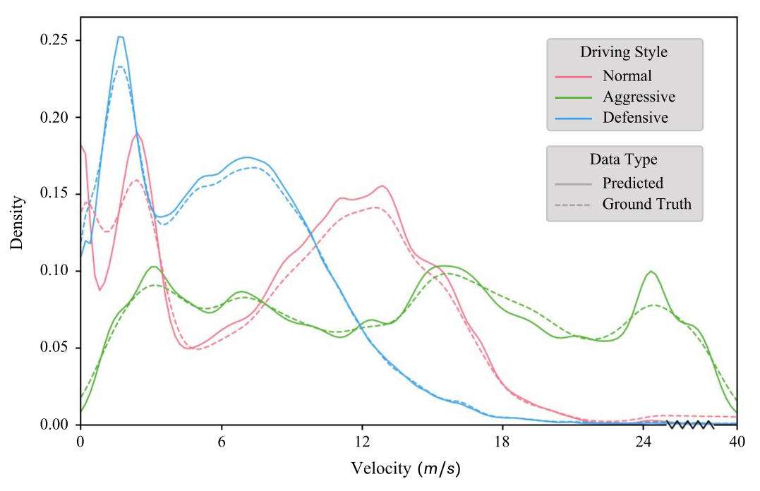
Figure 4 shows six selected scenarios, each retaining the camera context and pre/post-tuning BEV trajectories. Figure 5 shows predicted and recorded velocity-density profiles; aggressive behavior has more probability in the 24–40 m/s range. Matching speed distributions is evidence of stylization, not sufficient evidence of context-sensitive safety or comprehensive personal preference alignment.
| Method | Test Split | minADE | meanADE | minFDE | meanFDE | Diversity | BOE |
|---|---|---|---|---|---|---|---|
| w/o FT | Aggressive | 0.7546 | 1.5534 | 2.0054 | 4.3515 | 0.4419 | - |
| Aggr. SL | Aggressive | 0.5416 | 1.4485 | 1.3147 | 3.9245 | 0.5743 | 0.6577 |
| Aggr. RL | Aggressive | 0.5304 | 1.5036 | 1.2788 | 4.1039 | 0.6051 | 0.7660 |
| w/o FT | Defensive | 0.5538 | 1.4419 | 1.5854 | 4.3763 | 0.3741 | - |
| Defen. SL | Defensive | 0.3175 | 1.5317 | 0.8351 | 4.5239 | 0.3714 | 0.7430 |
| Defen. RL | Defensive | 0.3101 | 1.5309 | 0.8092 | 4.5603 | 0.3900 | 0.7922 |
| w/o FT | Normal | 0.2330 | 0.7734 | 0.5454 | 2.1207 | 0.3284 | - |
| Aggr. SL | Normal | 0.4612 | 1.3290 | 1.2850 | 3.8658 | 0.5276 | - |
| Aggr. RL | Normal | 0.3777 | 1.3034 | 1.0247 | 3.8057 | 0.5575 | - |
| w/o FT | Normal | 0.2330 | 0.7734 | 0.5454 | 2.1207 | 0.3284 | - |
| Defen. SL | Normal | 0.3675 | 3.0225 | 0.9428 | 8.7625 | 0.3811 | - |
| Defen. RL | Normal | 0.3361 | 2.5843 | 0.8537 | 7.4631 | 0.3773 | - |
5.3 Ablation Study
Table 3, referenced as Table 5 in the source prose, compares 810K, 3M, and 6M normal-training frames. minADE falls from 0.40 to 0.37 and minFDE from 0.87 to 0.81; meanFDE is non-monotonic, 2.67→2.70→2.66. Diversity drops from 0.28 to 0.26. More data improves several errors while concentrating the sampled distribution. Appendix C examines optimizer choice, cloning weight, and preference-data scale.
6 Conclusion
TrajHF demonstrates reward-driven movement toward two annotated driving styles and better minimum-error/style ratings than the tested supervised fine-tuning procedure. Its limitations include subjective and costly annotations, dependence on preference diversity, proprietary data, selected evaluation clips, weak isolation of the refresh stage, and normal-domain degradation. The paper identifies possible unsafe or biased personalization as a broader-impact concern. Neither its open-loop preference tests nor its separate PDMS-trained benchmark result provides a formal or general closed-loop safety guarantee.
Appendix A Details of Preferences Alignment Method
Appendix A explains how preferences are mined, how synthetic rejected trajectories are normalized, and how the reverse diffusion chain becomes the RL state-action process.
A.1 Preference Data Collection
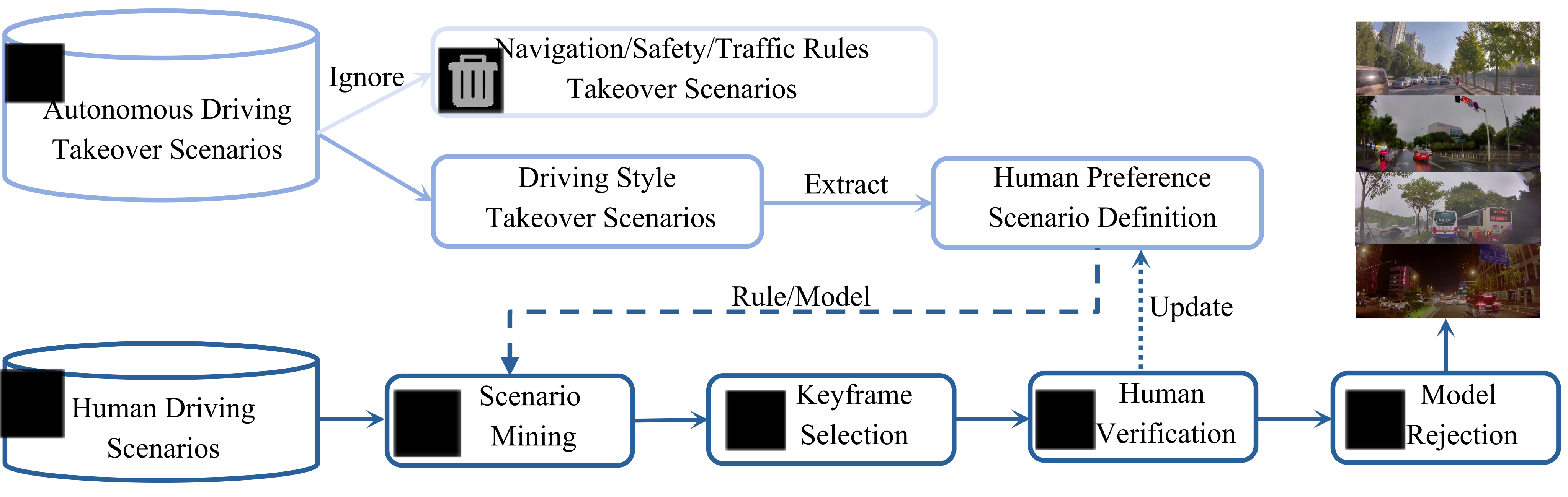
Takeover records are first separated into style-related cases and navigation/safety/traffic-rule interventions, which Figure 6 marks as ignored for preference definition. Style cases motivate six scenario categories, with examples such as overly aggressive or overly conservative behavior; all six categories are not enumerated. Rules or models mine similar human-driving scenes. Key frames capture the onset of a meaningful speed or direction decision, avoiding labels that occur too early or after the maneuver is already underway. Random manual verification revises definitions, and a baseline model rejects common cases already represented by ordinary driving. This process concentrates evaluation and training on departures from average behavior rather than random driving scenes.
A.2 Constructing semi-synthetic dataset for reward model training
For each chosen demonstration, three pretrained trajectories create candidate rejected pairs. A symmetric one-dimensional convolutional autoencoder, with two-layer encoder/decoder blocks and ReLU, reconstructs the rejected trajectories. Equation 12 combines geometric reconstruction with matching the chosen trajectory’s velocity mean and standard deviation; the prose calls these variances, while the equation explicitly uses standard deviations. The style weight is 0.3. This reduces low-level synthetic-versus-human differences that a reward model might exploit, but no reward-hacking ablation proves that those shortcuts are eliminated.
Equation 12
| (12) | ||||
A.3 RL Modeling Details
For a target style, observations and preferred trajectories come from its dataset. Gaussian initialization and stochastic denoising produce terminal trajectories, which receive a learned scalar reward.
Mixed sampling distribution 𝒫 θ .
Equation 13 defines the mixed rollout distribution as observation sampling, Gaussian initial noise, policy actions at each reverse-diffusion step, and deterministic state updates. A state contains the observation and current noisy trajectory; the action is the next, less noisy trajectory. The physical scene is held fixed during this internal denoising MDP.
Equation 13
| (13) |
Optimization objective.
Equation 14 maximizes expected reward of the final denoised trajectory. Equation 15 spells out the state, action, transition, policy, initial distribution, and terminal-only reward; Equation 16 gives the policy-gradient loss. These are optimization transitions within trajectory generation, not demonstrated interactions of the vehicle with a reactive environment.
Equations 14–16
| (14) |
| (15) |
| (16) |
Variance reduction.
Equation 17 first presents a critic-subtracted discounted advantage. The implemented group-relative approach then replaces that critic with normalized rewards from multiple candidate trajectories, avoiding critic warm-up and extra hyperparameters. This is the route from the generic policy-gradient derivation to the main DPGRPO objective.
Equation 17
| (17) |
Appendix B Details of Experiments
Appendix B specifies the inference selector, human evaluation, data capacities, training settings, and detailed interpretation of each qualitative example.
B.1 EM Algorithm for Trajectory Optimization
The EM-like selector begins with a randomly selected trajectory centroid and seeks representative coverage within distance d. Equations 18–21 retain the probability-weighted coverage objective and updates to weight, mean, and covariance, including hard-assignment language in the prose. The source uses x without a matching sample subscript in the mean update and does not fully specify d or initialization of candidate probabilities/covariances. These equations describe the intended aggregation but are not a complete executable recipe. NavSim uses 25 iterations per scenario.
Equations 18–21
| (18) |
| (19) | ||||
| (20) | ||||
| (21) |
B.2 Human Preference BOE
Geometric errors may penalize speed or lateral differences without revealing whether an overtaking decision matches the desired style. Five professional driving-style annotators therefore compare paired trajectories in context without seeing model identity, choosing the first, second, or a tie. Equation 22 gives BOE: a model’s wins plus ties divided by evaluated scenes, averaged across annotators. Two models’ BOEs need not sum to one because both receive credit for ties.
The study manually selects 53 aggressive and 151 defensive test clips where pretraining already deviates from the intended style. These are diagnostic difficult cases, not an unbiased estimate across the test distribution. The paper does not report tie frequency, annotator agreement, confidence intervals, or individual-driver preference heterogeneity.
Equation 22
| (22) |
B.3 Internal Data Capacities
Table 4 lists normal-data scales of 65,628/298,706/487,812 clips and 810K/3M/6M frames. Aggressive preference data contain 2,967 clips and 35,329 frames; defensive data contain 49,030 clips and 136,782 frames. These unequal capacities contextualize the two styles’ results. The table reports split capacities without a full train/test allocation or leakage audit.
| Data Split | Clips | Frames |
|---|---|---|
| small | 65,628 | 810K |
| medium | 298,706 | 3M |
| large | 487,812 | 6M |
| aggressive | 2967 | 35329 |
| defensive | 49030 | 136782 |
B.4 Implementation Details
A base ViT encodes concatenated 1024 × 256 front-view images, and ResNet34 encodes 256 × 256 LiDAR inputs. Ten stochastic denoising steps are used in training and inference; outputs have eight waypoints over four seconds. Base training uses Adam, OneCycle scheduling, learning rate 10⁻⁴, batch size 512 across eight H20 GPUs, and 1,000 NavSim epochs. The reconstruction autoencoder uses learning rate 10⁻³, batch 32, and 100 epochs; the reward model uses margin 1, learning rate 2 × 10⁻⁵, batch 32, and up to 30 epochs with early stopping.
NavSim score-based fine-tuning runs 45 epochs on sixteen H20 GPUs, batch 16 per GPU, cloning weight 0.01, and learning rates 6 × 10⁻⁵ for ViT and 5 × 10⁻⁵ elsewhere. Internal style adaptation uses K=8, discount 0.99, cloning weight 0.1, and learning rate 5 × 10⁻⁵. SL runs 200 epochs at batch 128; RL runs 20 at batch 32, followed by a 100-epoch supervised refresh using the SL settings. The refresh is therefore substantial despite being described as short. Inference latency and a resource-matched comparison of SL versus the complete RL-plus-refresh pipeline are not reported.
B.5 Qualitative Analysis
The three aggressive examples show borrowing an opposite lane to pass vulnerable road users and a parked vehicle, increasing overtaking speed, and changing lanes around a slow vehicle. The defensive examples show slowing near an ambiguous intersection, slowing at night, and yielding space to an overtaking large vehicle. All image panels, trajectory overlays, and legends remain intact. These are selected planned trajectories, with no closed-loop collision or human-comfort measurement for the pictured maneuvers.
Appendix C Supplementary Ablation Experiments
The supplementary experiments test alternative preference optimizers, reference-policy regularization, and smaller preference datasets. All reported numerical rows are retained.
C.1 Ablation for PPO Variants
Because the cited PPO driving method [29] is not publicly available, the authors reimplement it. PPO gives worse minimum preference errors than DPGRPO but sometimes better mean errors and less degradation on normal data: for example aggressive normal minADE is 0.2716 for PPO versus 0.3777 for DPGRPO. It reflects an adaptation/retention tradeoff, not uniform dominance. The proposed explanations involving restrictive clipping and multimodal collapse are conjectures rather than separately tested mechanisms.
The DPO [42] ablation reports only the aggressive case, with minADE 4.9720, minFDE 10.2502, and reduced diversity 0.1835. This shows failure of the tested implementation/setup, not that DPO is universally ineffective for driving preferences. No equivalent hyperparameter sweep, repeated-run uncertainty, or defensive DPO result is supplied.
| Method | Test Split | minADE | meanADE | minFDE | meanFDE | Diversity |
|---|---|---|---|---|---|---|
| Aggr. PPO | Aggressive | 0.7099 | 1.5640 | 1.7958 | 4.2434 | 0.4704 |
| Aggr. PPO | Normal | 0.2716 | 0.8546 | 0.6518 | 2.3182 | 0.3397 |
| Defensive PPO | Defensive | 0.4638 | 1.3630 | 1.2667 | 4.1038 | 0.3754 |
| Defensive PPO | Normal | 0.3314 | 1.1452 | 0.8002 | 3.1791 | 0.3346 |
C.2 Ablation for BC Loss Weight
Across cloning weights from 1 to 0.001, 0.1 gives the best minimum displacement errors for both styles. Other objectives prefer different weights: aggressive diversity is highest at 0.01, and defensive meanADE/meanFDE are best at 0.5. Thus 0.1 is a favorable best-case-error compromise rather than the optimum for every metric. The full table exposes this tradeoff.
| Data Split | minADE | meanADE | minFDE | meanFDE | Diversity | |
|---|---|---|---|---|---|---|
| 1.0 | Aggressive | 0.5535 | 1.5238 | 1.3422 | 4.1555 | 0.6035 |
| 0.5 | Aggressive | 0.5635 | 1.5747 | 1.3694 | 4.2782 | 0.6088 |
| 1e-1 | Aggressive | 0.5304 | 1.5036 | 1.2788 | 4.1039 | 0.6051 |
| 1e-2 | Aggressive | 0.5585 | 1.5697 | 1.3479 | 4.2692 | 0.6142 |
| 1e-3 | Aggressive | 0.5330 | 1.5332 | 1.2805 | 4.1650 | 0.6131 |
| 1.0 | Defensive | 0.3187 | 1.5219 | 0.8418 | 4.5173 | 0.3763 |
| 0.5 | Defensive | 0.3252 | 1.4671 | 0.8579 | 4.3304 | 0.3758 |
| 1e-1 | Defensive | 0.3101 | 1.5309 | 0.8092 | 4.5603 | 0.3900 |
| 1e-2 | Defensive | 0.3209 | 1.4827 | 0.8389 | 4.3797 | 0.3755 |
| 1e-3 | Defensive | 0.3195 | 1.5972 | 0.8368 | 4.6734 | 0.3782 |
C.3 Ablation of data scales of DPGRPO
Increasing preference data from 10% to 50% sharply reduces displacement errors; 100% improves them further by smaller amounts. Aggressive minADE changes 0.7025→0.5431→0.5304; defensive minADE changes 0.4483→0.3352→0.3101. Diversity is non-monotonic and sometimes higher with less data. Three sampled budgets suggest diminishing gains but do not establish a fitted logarithmic scaling law or the uncertainty from different random subsets.
| Method | Scale | Test Split | minADE | meanADE | minFDE | meanFDE | Diversity |
|---|---|---|---|---|---|---|---|
| Aggr. RL | 10% | Aggr. | 0.7025 | 2.1477 | 1.6146 | 5.5560 | 0.6437 |
| Aggr. RL | 50% | Aggr. | 0.5431 | 1.5623 | 1.3091 | 4.2650 | 0.6015 |
| Aggr. RL | 100% | Aggr. | 0.5304 | 1.5036 | 1.2788 | 4.1039 | 0.6051 |
| Defen. RL | 10% | Defen. | 0.4483 | 1.8836 | 1.1182 | 5.2600 | 0.3746 |
| Defen. RL | 50% | Defen. | 0.3352 | 1.5785 | 0.8638 | 4.6677 | 0.4014 |
| Defen. RL | 100% | Defen. | 0.3101 | 1.5309 | 0.8092 | 4.5603 | 0.3900 |