At a glance
LUMOS trains a language-conditioned robot policy inside a learned world model. The model first learns dynamics from offline play; an actor–critic then practices latent rollouts, receiving rewards for matching demonstration trajectories. Hindsight goal relabeling, latent plans, and contrastive language alignment allow sparsely annotated play to support language commands.
At matched 64×64 image resolution, LUMOS completes an average 2.34 instructions in CALVIN chains versus HULC’s 2.27. Physical experiments report 2.05 versus 1.90 sequential tasks. “Zero-shot” here means no online policy fine-tuning after offline training on real robot data, not transfer without real-world experience. Project videos, dataset, and code accompany the paper.
I Introduction
Behavior cloning learns actions on demonstrated states, but small deployment mistakes can lead to unfamiliar observations and compound over time. Practicing a policy under its own state distribution can address this mismatch; doing so physically is expensive.
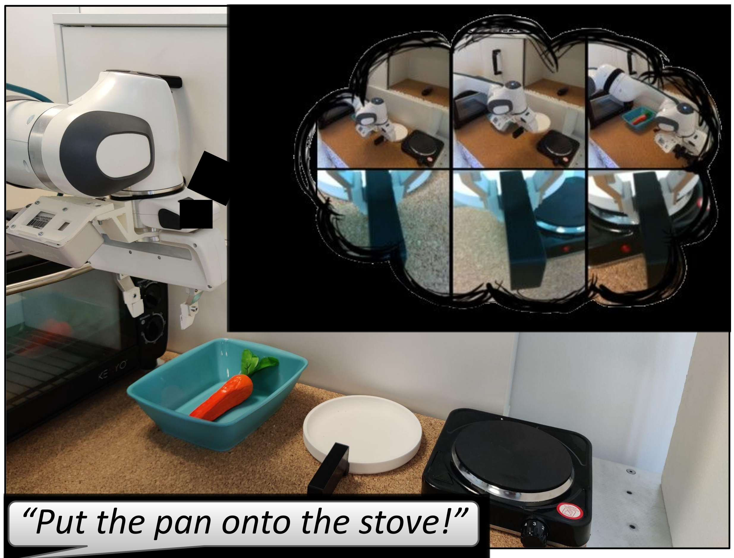
LUMOS practices in an action-conditioned latent simulator learned from play data. It extends DITTO trajectory matching with language conditioning and hindsight latent planning. The proposed benefit is recovery over multiple imagined steps rather than independent action prediction.
This substitutes learned dynamics for a hand-built simulator, but does not eliminate modeling error or guarantee recovery on real states outside the dataset. The experiments show a proof of concept on specified tabletop tasks, not unrestricted long-horizon language execution.
II Related Work
MCIL learns language-steerable skills from sparsely labeled play. HULC adds latent planning and language–vision contrastive alignment; other systems add affordances, explicit skill decompositions, or diffusion policies. LUMOS studies a different source of improvement: on-policy learning inside a fixed offline world model.
Hindsight planning gives a training-time recognizer the entire demonstration, then teaches a proposal network to predict a useful plan from the current state and goal. At inference only the proposal is available. This compresses multi-step behavior without assuming one unique trajectory for every start/goal pair.
Dreamer-style recurrent models provide compact predictive states. DITTO rewards similarity to expert latent trajectories and trains an actor–critic through imagined dynamics. LUMOS combines these components; its baseline experiment does not compare against every newer diffusion, affordance, or hybrid control system.
III Problem Formulation
The setting is goal-conditioned imitation under partial observability: the robot sees camera images, takes continuous pose commands plus a gripper command, and has no usable task-reward feedback for offline policy training.
Fixed play trajectories are sampled into windows and retrospectively labeled with their final reached state as a goal. A small subset also has free-form language descriptions. These two goal modalities train a common policy; the language labels describe behavior already present in the data rather than generating new demonstrations.
IV LUMOS
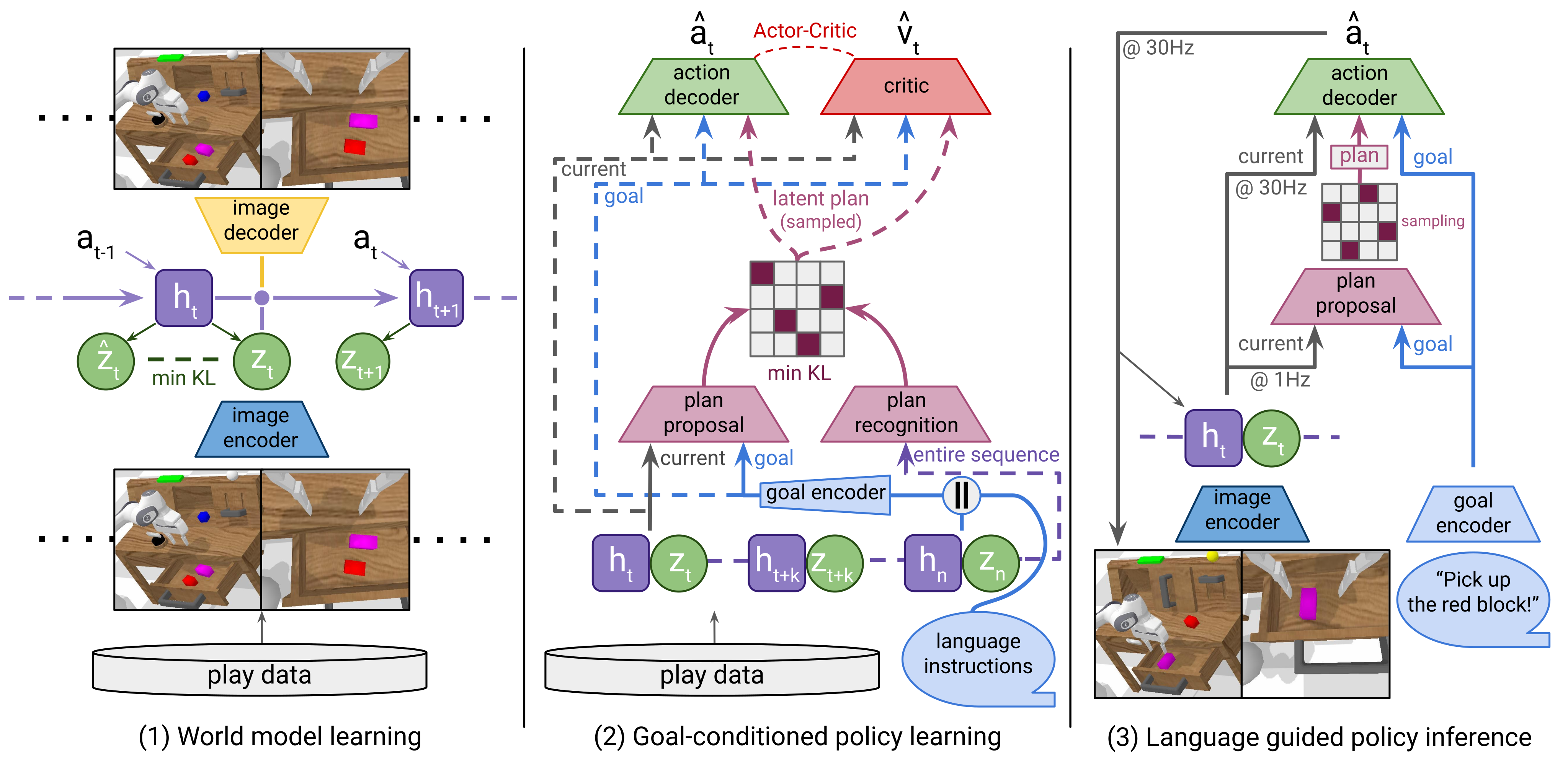
Training has two stages. Fit the world model to play observations and actions, then freeze it while optimizing the policy through imagined latent trajectories. At execution, current camera observations update the model state and a language instruction supplies the goal.
IV-A World Model Learning
Separate convolutional encoders and decoders process static and gripper-camera images. Their features feed a DreamerV2 recurrent state-space model with deterministic recurrent memory and stochastic categorical latent variables.
The posterior sees the current observation; the prior predicts the next latent state from history and actions without that observation. Training combines reconstruction and KL regularization, using straight-through gradients for categorical samples. The retained module definitions and objective specify this structure.
Imagined rollouts use prior predictions after an initial state estimate. They are cheap to generate, but their quality remains bounded by learned dynamics and dataset coverage. “Unlimited” model rollouts do not provide unlimited reliable real-world experience.
Equations 1–2
| (1) |
| (2) |
IV-B Behavior Learning
The policy encodes the world-model trajectory into perceptual features. A transformer plan recognizer sees the complete training window and produces categorical latent plans; a proposal network learns to predict their distribution from the initial state and goal. At test time it supplies the plan without future observations.
For language-labeled windows, a symmetric contrastive objective aligns latent-trajectory and sentence embeddings, treating corresponding pairs as positives and other batch pairs as negatives. Unlabeled windows use reached-state goals and omit the language contrastive term.
The intrinsic reward is the expert/agent latent inner product divided by the squared larger latent norm. It favors aligned, similarly scaled states at corresponding times. Equation 3 contains no separate action-distance term, despite the prose’s state–action matching description. This surrogate encourages imitation within the model; it is not an observed task-success reward.
A feed-forward actor outputs a tanh-transformed Gaussian from current features, goal, and sampled plan. A critic predicts discounted intrinsic returns. The critic fits bootstrapped lambda returns with stopped target gradients, while the actor differentiates through frozen model dynamics to increase return and also minimize plan-KL and language-alignment losses.
This creates on-policy experience in the learned model, not new online robot data. It can reduce action-error accumulation relative to the tested cloning ablation, but model errors can still produce apparently rewarding imagined behavior that fails physically.
Equations 3–4
| (3) |
| (4) | ||||
| Method | No. Instructions in a Row (1000 chains) | |||||
|---|---|---|---|---|---|---|
| 1 | 2 | 3 | 4 | 5 | Avg. Len. | |
| GCBC [9] | 56.7% (3.4) | 20.9% (1.9) | 7.3% (2.9) | 1.6% (0.5) | 0.04% (0.0) | 0.63 (0.4) |
| MCIL [11] | 70.3% (3.1) | 40.2% (2.9) | 21.6% (4.1) | 11.1% (1.9) | 5.4% (1.0) | 1.48 (0.3) |
| HULC [10] | 77.6% (1.1) | 58.05% (0.3) | 41.6% (1.3) | 29.8% (0.9) | 20.0% (1.5) | 2.27 (0.05) |
| LUMOS (ours) | 80.7% (1.0) | 59.3% (1.4) | 42.6% (1.8) | 30.7% (1.2) | 21.1% (0.8) | 2.34 (0.05) |
| No DITTO | 71.8% (1.3) | 45.6% (1.5) | 27.8% (1.9) | 14.2% (1.8) | 8.7% (0.7) | 1.68 (0.02) |
| No latent plan | 76.5% (2.5) | 50.5% (0.9) | 28.7% (1.3) | 15.9% (0.8) | 11.0% (0.7) | 1.81 (0.01) |
| No alignment | 73.3% (1.5) | 52.6% (0.9) | 39.8% (2.0) | 27.3% (1.3) | 17.2% (0.9) | 2.05 (0.06) |
Equations 5–6
| (5) |
| (6) |
V Experimental Results
Evaluation separates CALVIN instruction chaining, component ablations, and transfer of offline-trained policies to a real tabletop robot.
V-A Experiments in Simulation
The simulation study trains and evaluates in CALVIN environment D, using six hours of play, 34 subtasks, and about 1% language annotation. Each of three seeds is evaluated on 1,000 chains of up to five instructions. This is not the harder cross-environment ABC→D generalization protocol.
All methods receive two 64×64 camera streams. LUMOS has 80.7% first-task success, 21.1% five-task completion, and average chain length 2.34±0.05. HULC has 77.6%, 20.0%, and 2.27±0.05. Parentheses in the original table are standard deviations across three seeds, not confidence intervals. The aggregate improvement is modest and should not be presented as a broad benchmark-state-of-the-art claim.
Replacing intrinsic-reward practice with mean-squared-error cloning lowers mean chain length to 1.68; removing latent plans gives 1.81, and removing language alignment gives 2.05. These controlled ablations support the combined training design, without independently measuring distribution shift.
The source table contains one numerical inconsistency: GCBC’s reported completion probabilities sum to about 0.865 expected tasks, whereas its printed average length is 0.63. Both original entries remain unchanged; no corrected baseline value is inferred.
Figure 3 is a qualitative prediction check: five observed frames initialize a held-out trajectory, then known actions drive 195 predicted steps. The model trains on 50-step windows. Visual plausibility in this example is not a quantitative guarantee of long-horizon state or task accuracy.

V-B Experiments in Real-World
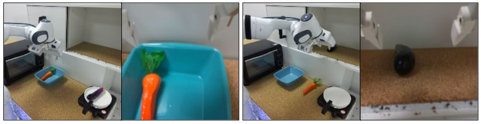
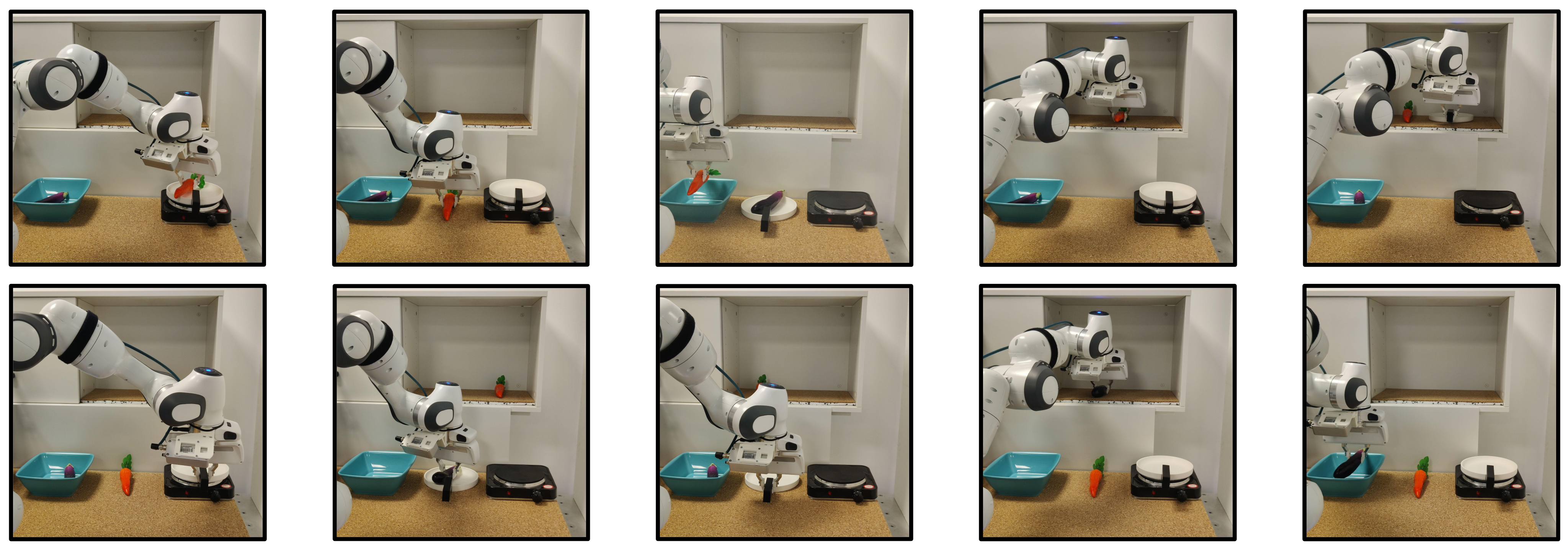
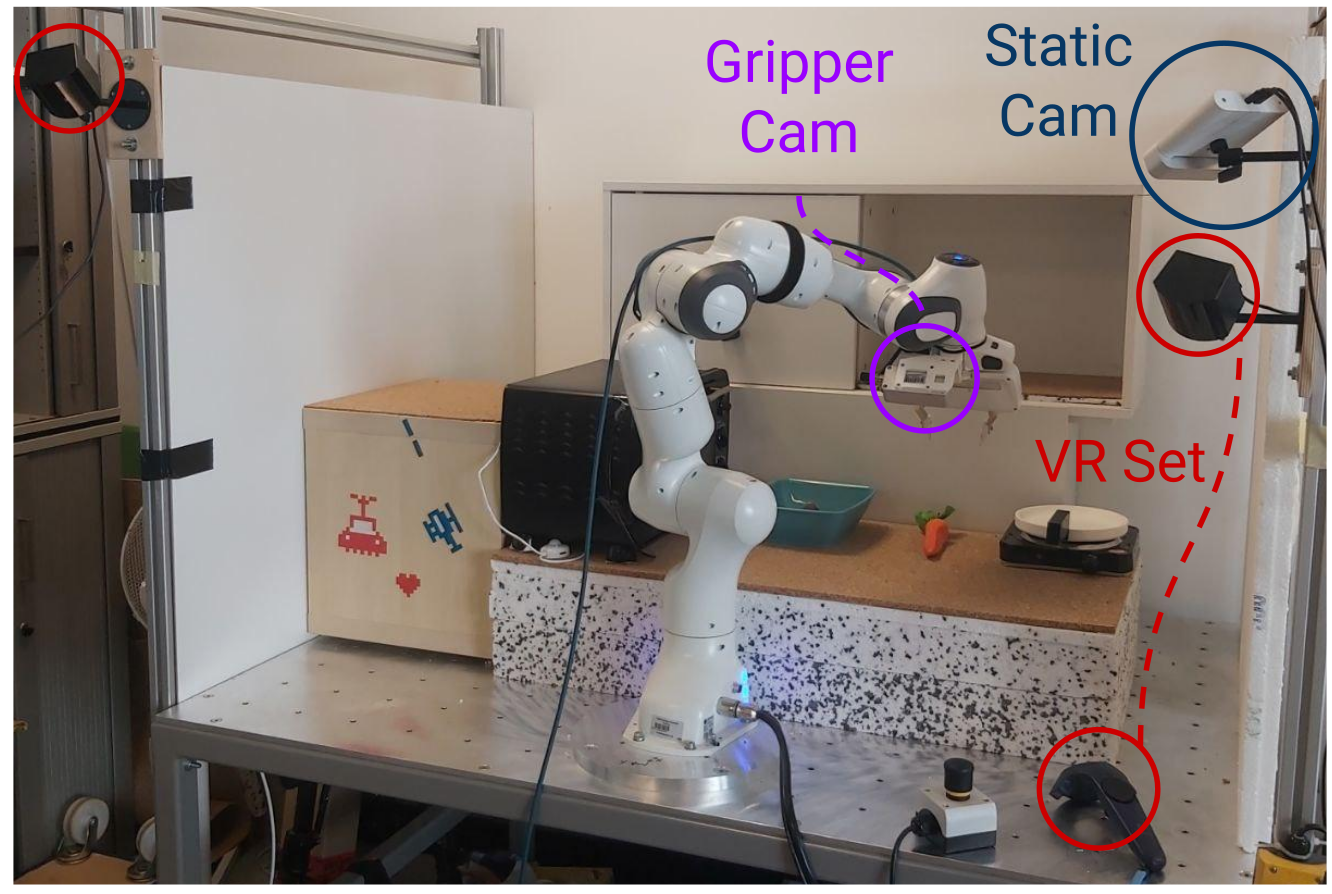
The real setup uses a Panda arm with a stove, bowl, cabinet, pan, and toy carrot/eggplant. Three hours of teleoperated play train the world model and policy; roughly 2,800 sampled windows receive language descriptions. The paper calls this less than 1% of data but does not define the overlapping-window denominator, so it should not be read as a percentage of unique recorded frames.
Each task is tested in 20 rollouts from neutral starting configurations. Vegetable tasks are evaluated separately for carrot and eggplant and then merged for display; choosing the wrong vegetable is a failure. The table’s 67.68% LUMOS and 63.39% HULC averages are means across the 14 displayed grouped rows, not necessarily the same weighting as all individual tasks.
LUMOS is better on many tasks but not all: lifting the pan from the table is 65% versus HULC’s 75%, and placing a vegetable in the pan is 62.5% versus 65%. Both methods reach only 35% when lifting the pan from the cabinet. Across 20 five-instruction chains, mean length is 2.05 versus 1.90.
The model-predicted table average, 75.89%, exceeds physical performance, exposing a model-to-real gap; individual simulated outcomes are not uniformly better. The paper supplies no real-world repeated-seed uncertainty. Neutral starts reduce task/start correlations but do not prove language is the only usable cue.
| Task / Method | LUMOS (ours) | HULC [10] | World Model |
|---|---|---|---|
| Lift the vegetable from the table | 67.5% | 62.5% | 72.5% |
| Lift the vegetable from the pan | 75% | 72.5% | 77.5% |
| Lift the vegetable from the bowl | 72.5% | 67.5% | 75% |
| Lift the vegetable from the cabinet | 55% | 50% | 70% |
| Lift the pan from the table | 65% | 75% | 70% |
| Lift the pan from the stove | 80% | 70% | 75% |
| Lift the pan from the cabinet | 35% | 35% | 60% |
| Place the vegetable onto the table | 90% | 85% | 92.5% |
| Place the vegetable onto the pan | 62.5% | 65% | 77.5% |
| Place the vegetable into the bowl | 85% | 75% | 80% |
| Place the vegetable into the cabinet | 70% | 60% | 77.5% |
| Place the pan onto the table | 70% | 65% | 80% |
| Place the pan onto the stove | 65% | 55% | 85% |
| Place the pan into the cabinet | 55% | 50% | 70% |
| Average over tasks | 67.68% | 63.39% | 75.89% |
| Average no. of sequential tasks | 2.05 | 1.90 | - |
VI Conclusion and Limitations
LUMOS shows that a policy can learn language-guided tabletop skills through a fixed world model and then execute without online fine-tuning. Its strongest evidence is the within-architecture ablation, while comparisons with HULC show smaller aggregate gains.
The main limitations are uncertain model fidelity, restricted data/environment coverage, and expensive higher-resolution world modeling. Offline real data remain necessary. Increasing rollout length alone cannot solve missing dynamics or guarantee robust physical recovery.
VII Appendix
The appendix specifies world-model and policy architectures, optimization settings, baseline modifications, robot actions, and real-data collection. All parameter tables and mathematical details are retained.
VII-A Hyperparameters and Training Details of the World Model
The world model has about 40 million parameters. Its 1,024-dimensional recurrent state is concatenated with a flattened 32-by-32 categorical sample, giving 2,048 latent dimensions. Training uses batch size 50 and 50-step sequences, reconstruction/KL scale 0.3, learning rate 3×10⁻⁴, gradient clipping 100, and the remaining settings in Table III.
Training samples windows from long play episodes and randomly resets recurrent state with probability 0.01, encouraging use of current observations as well as history.
Equation 7’s printed KL-balancing weights conflict with its explanation: delta=0.8 weights the posterior-update term by 0.8 and prior-update term by 0.2, whereas the prose says the prior should update faster. The original equation and table are retained; the implemented convention is not established by this text.
Equation 7
| (7) |
| Name | Symbol | Value |
|---|---|---|
| Batch size | 50 | |
| Sequence length | 50 | |
| Deterministic latent state dimensions | — | 1024 |
| Discrete latent state dimensions | — | 32 |
| Discrete latent state classes | — | 32 |
| Latent dimensions | 2048 | |
| KL loss scale | 0.3 | |
| KL balancing | 0.8 | |
| RSSM reset probability | ||
| World model learning rate | — | |
| Gradient clipping | — | 100 |
| Adam epsilon | ||
| Weight decay (decoupled) | — |
VII-B Hyperparameters and Training Details of the Agent
The perceptual encoder maps 2,048-dimensional latent states through two fully connected layers, with hidden size 1,024 and output size 128. The text encoder is paraphrase-MiniLM-L3-v2, producing 384-dimensional sentence vectors; goal encoders map image/latent or language inputs to 32 dimensions.
Plan recognition uses two transformer blocks, eight heads, and hidden size 2,048. Plan proposal has four 2,048-unit fully connected layers. Plans use 32 categorical variables with 32 classes each. Their KL loss uses the same balancing convention whose printed direction is ambiguous in Appendix A.
Contrastive alignment normalizes latent/text features, scales their pairwise similarities by an exponentiated learned temperature, and averages cross-entropies in both retrieval directions. Only matching diagonal pairs are positive; semantically equivalent instructions elsewhere in the batch can still act as negatives under this rule.
The actor has eight 256-unit layers, about one million parameters, versus roughly 15 million in the described HULC action decoder. This is an action-decoder comparison, not total-system model size: LUMOS additionally uses the roughly 40-million-parameter world model. The critic has eight 1,024-unit layers.
Agent windows are sampled at lengths 20–32 and padded to 32; batch size is 512. Table IV specifies plan-KL scale 0.1, contrastive scale 3.0, discount 0.995, lambda 0.95, actor/critic learning rates 2×10⁻⁴/3×10⁻⁴, and slow-critic updates every 100 steps.
Lambda returns mix immediate rewards with recursive bootstrapped values. At lambda=1 the printed finite-horizon recurrence still ends in a learned value estimate, so the source’s “unbiased Monte Carlo” description requires additional terminal-value assumptions. The formula remains intact.
| Name | Symbol | Value |
| Batch size | 512 | |
| Sequence length | 32 | |
| Minimum window length | — | 20 |
| Maximum window length | — | 32 |
| Feature dimensions | 128 | |
| Latent goal dimensions | 32 | |
| Discrete latent plan dimensions | — | 32 |
| Discrete latent plan classes | — | 32 |
| KL loss scale | 0.1 | |
| Contrastive loss scale | 3.0 | |
| KL balancing | 0.8 | |
| Discount factor | ||
| parameter | ||
| Optimizer | — | Adam |
| Actor learning rate | — | |
| Critic learning rate | — | |
| Slow critic update interval | — |
Equations 8
| (8) |
VII-C Modifications to Baselines for Fair Comparisons
To match the 64×64 inputs, baseline convolution kernels/strides change from 8/4, 4/2, 3/1 to 4/2, 2/2, 2/2. Baseline images receive random shifts of 0–3 pixels with bilinear interpolation; LUMOS does not use this image augmentation.
These changes equalize input resolution but differ from original higher-resolution baseline configurations. The comparison supports the reported compute-conscious setup, not the best attainable performance of each baseline at its original resolution.
VII-D 7-DoF Action Framework
Actions contain three relative translations, three base-frame Euler-angle changes, and one gripper value. Pose values lie in [−1,1]; the actor also treats the gripper output continuously before thresholding.
The appendix gives incompatible gripper conventions: it first says −1 opens and +1 closes, then says positive outputs open and nonpositive outputs close. Both statements are preserved here as a source ambiguity; a reproducer must verify the actual controller mapping before execution. The paper also does not give physical translation/rotation scaling in this paragraph.
Equation
VII-E Data Collection Details
Three hours of play were recorded using HTC VIVE Pro teleoperation. The dataset includes proprioception, absolute commanded actions, and 200×200 static Azure Kinect and gripper-mounted FRAMOS D435e RGB observations. Training derives relative actions by differencing consecutive absolute commands and resizes images to 64×64.
Recorded data are downsampled from 30 Hz to 15 Hz. Figure 2 labels inference at 30 Hz, while the appendix does not explain rate conversion between training actions and execution. These data-collection details qualify the zero-online-learning claim; the system still learns from substantial recorded physical interaction.