At a glance
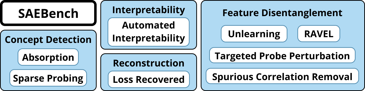
SAEBench evaluates sparse autoencoders (SAEs) with eight complementary metrics covering reconstruction, concept detection, interpretability, and feature disentanglement. Across more than 200 SAEs, improvements on the usual sparsity–reconstruction trade-off do not reliably predict practical usefulness. Hierarchical Matryoshka SAEs perform particularly well on several concept-isolation measures despite weaker reconstruction scores. Architecture, dictionary width, sparsity, model, and layer all affect the results.
1 Introduction
An SAE should recover understandable, independently usable features from model activations. Reconstruction and sparsity are convenient training objectives, but neither guarantees those properties: features can split, combine, or absorb one another. SAEBench brings several diagnostic and intervention-based tests into one reproducible framework, including two new measures of concept separation.
2 Related work
2.1 SAEs for Interpretability
An SAE encodes an activation vector into a sparse higher-dimensional representation and linearly decodes it. The original ReLU architecture balances reconstruction error against an L1 sparsity penalty. Later methods change the architecture, activation rule, or loss. These changes improve proxy objectives, but an arbitrarily wide dictionary could reconstruct perfectly with one active latent while providing little explanatory value.
Equations 1–3
| (1) | ||||
| (2) | ||||
| (3) |
2.2 SAE Evaluations
Prior evaluations test isolated properties: automated feature explanations, sparse concept probes, board-game features with ground truth, or supervised comparison dictionaries. Each is useful, but none alone captures overall SAE quality. The benchmark combines these perspectives rather than declaring a single universal winner.
3 SAEBench: A Comprehensive Benchmark
The framework is designed for diverse metrics, extensibility, automation, reproducibility, and roughly one-to-two-hour evaluation runs per SAE. Cached activations and probes reduce repeated setup costs. These runtime targets depend on model and dictionary size.
3.1 Metrics
The eight metrics cover four goals: detect concepts with few latents, produce understandable feature descriptions, reconstruct the model’s behavior, and separate concepts for selective interventions. Some non-SAE baselines outperform SAEs on particular tests. That is useful evidence about limitations, rather than a reason to remove those tests.
3.2 Existing Metrics
3.2.1 Traditional Sparsity–Fidelity Tradeoff
Sparsity is measured by the number of active latents. Loss recovered compares the model’s next-token loss after replacing an activation with its SAE reconstruction against the original model and a zero-ablation baseline. This measures behavioral fidelity, but does not establish that the recovered representation is understandable or disentangled.
Equation 4
| (4) |
3.2.2 Automated Interpretability
An LLM describes a latent from activating examples, then predicts which held-out sequences activate it. Prediction accuracy provides the automated interpretability score. The result measures the usefulness of this generated explanation on the selected examples, rather than directly measuring human understanding.
3.2.3 k -Sparse Probing
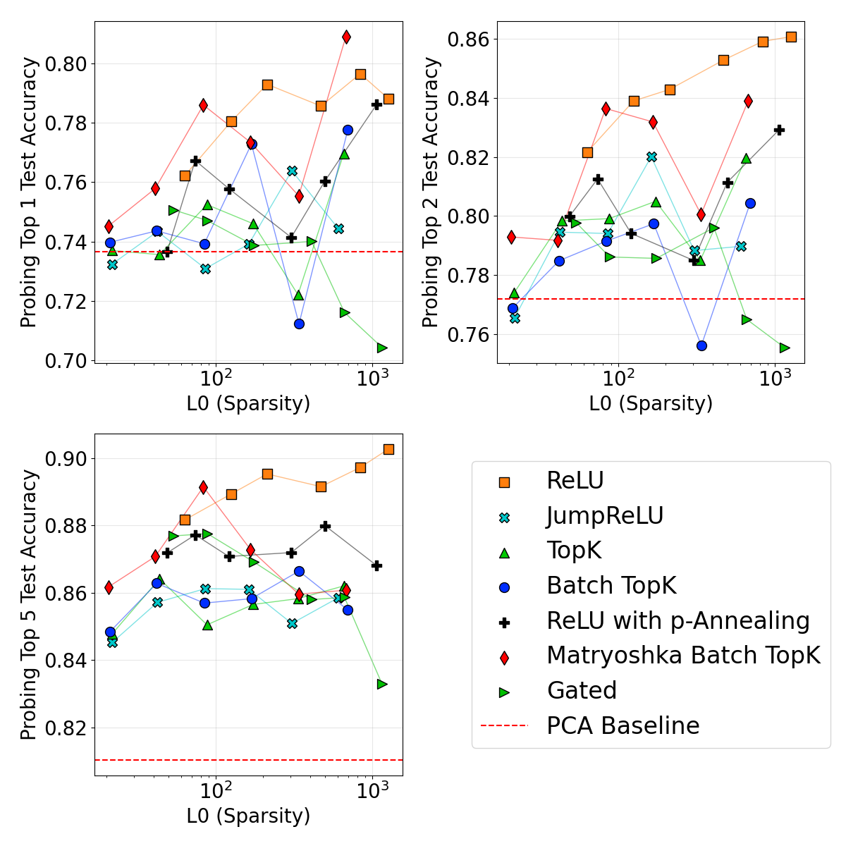
For each labeled concept, the evaluation selects latents with the largest positive–negative mean activation difference and trains a linear classifier using only those latents. It tests one, two, and five latents, emphasizing one-latent probes in the main results. Strong performance indicates that a specified concept is accessible through a small feature set.
3.2.4 RAVEL
RAVEL tests whether latent interventions change one entity attribute while preserving others—for example, changing a city’s country without changing its language. A learned binary mask transfers selected latent values from a source entity to a target. The score averages successful intended changes and preservation of unrelated attributes [19].
3.3 Adapted Metrics
Two existing research tools are adapted into systematic evaluations: detecting feature absorption and selectively suppressing knowledge.
3.3.1 Feature Absorption
Sparsity can encourage a broad concept to become “the broad concept except its subtype,” because the subtype latent already supplies the shared information. The absorption test examines first-letter features and detects cases where other latents compensate for a main feature’s missing or weakened activation. The revised metric allows partial absorption and multiple compensating latents across model layers.
3.3.2 Unlearning Capability
The unlearning test selects latents frequent in biology text but infrequent in a retain set, then clamps active selected latents to negative values. It measures reduced WMDP-bio accuracy while requiring unrelated MMLU performance to remain high. This tests selective intervention effectiveness; a reduced score on these questions does not establish permanent erasure of all biological knowledge.
3.4 Novel Metrics
Spurious Correlation Removal (SCR) starts with a classifier trained on a biased dataset, then zero-ablates selected SAE latents associated with the unwanted correlation. Better classification on balanced data indicates more selective removal. Targeted Probe Perturbation (TPP) asks whether ablating latents important to one class harms that class’s probe while sparing other classes. Both extend the feature-ablation approach of sparse feature circuits [25].
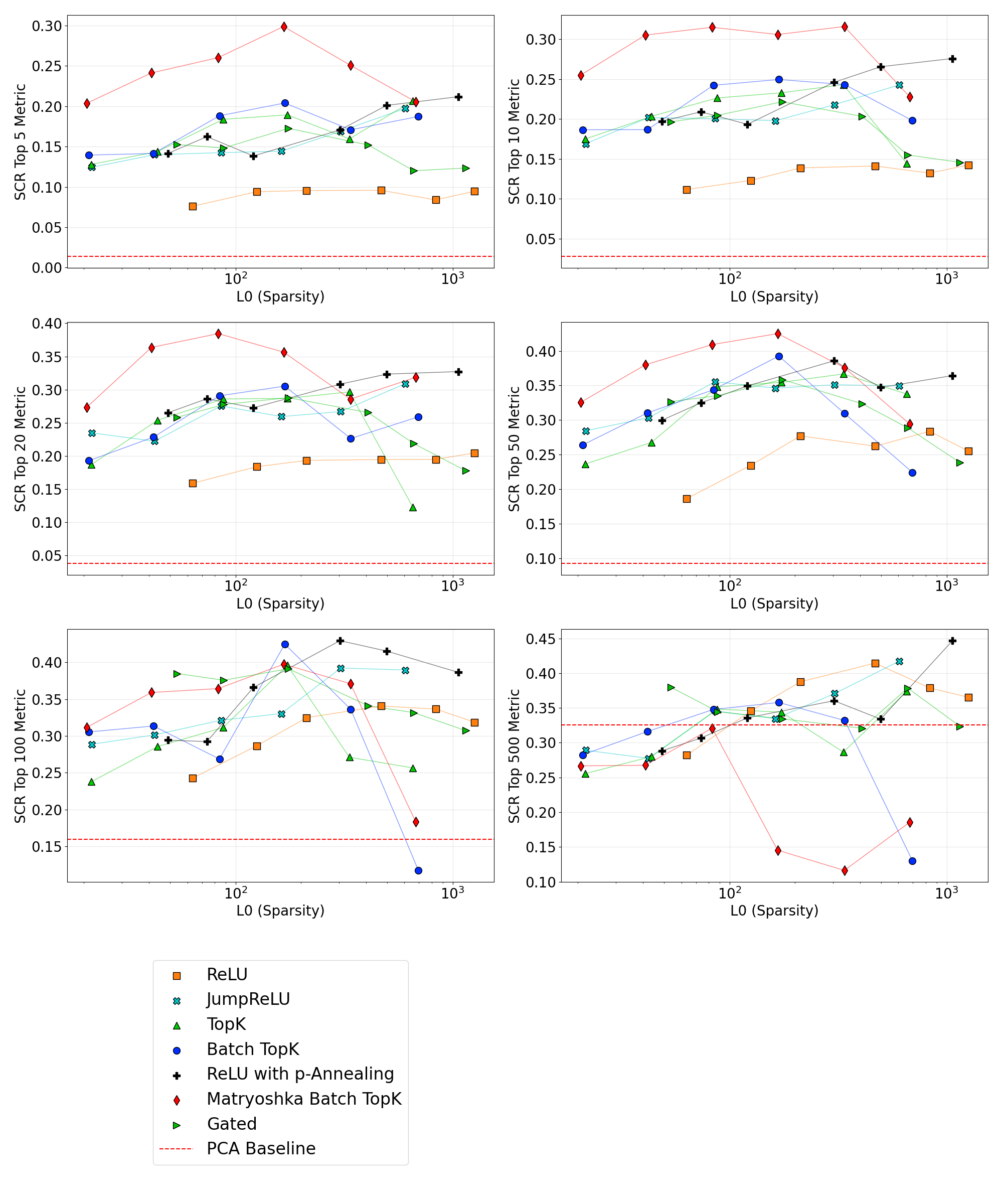
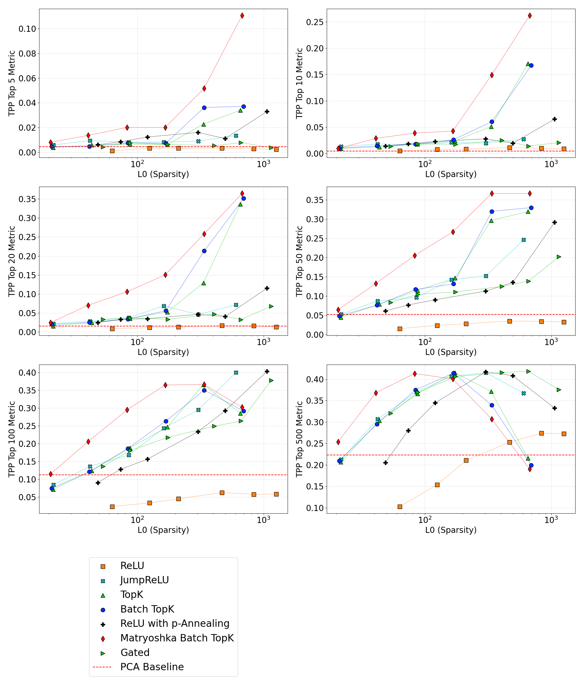
These tests address completeness and isolation: whether a small latent set captures a concept sufficiently well to remove its effect, without removing unrelated concepts. The study varies intervention size from 5 to 500 latents and emphasizes 20 as a manageable manual-analysis budget.
3.5 Practitioner’s Guide
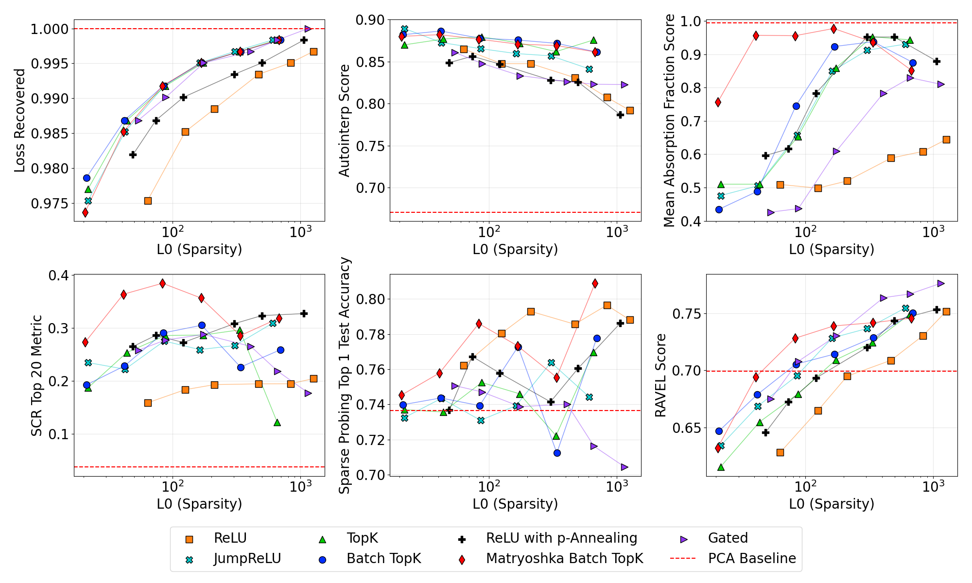
Compare architectures over a range of actual sparsities, with otherwise matched training settings. An apparent gain at one operating point may merely reflect a different number of active latents. The authors recommend examining the attainable trade-offs on the metrics relevant to the intended application.
4 Results
The main suite varies seven SAE approaches, dictionary widths of roughly 4,000–65,000 latents, and a broad range of active-latent counts on middle-layer activations of Gemma-2-2B and Pythia-160M. Additional Gemma Scope evaluations extend to million-latent dictionaries and a nine-billion-parameter model. Most detailed comparisons emphasize Gemma-2-2B at 65,000 latents.
| Evaluated SAE Architectures |
| ReLU (Anthropic Interpretability Team, 2024a) |
| MatryoshkaBatchTopK (Bussmann et al., 2024b) |
| TopK (Gao et al., 2024) |
| BatchTopK (Bussmann et al., 2024a) |
| Gated (Rajamanoharan et al., 2024a) |
| JumpReLU (Rajamanoharan et al., 2024b) |
| P-Annealing (Karvonen et al., 2024) |
4.1 Comparing SAE Architectures
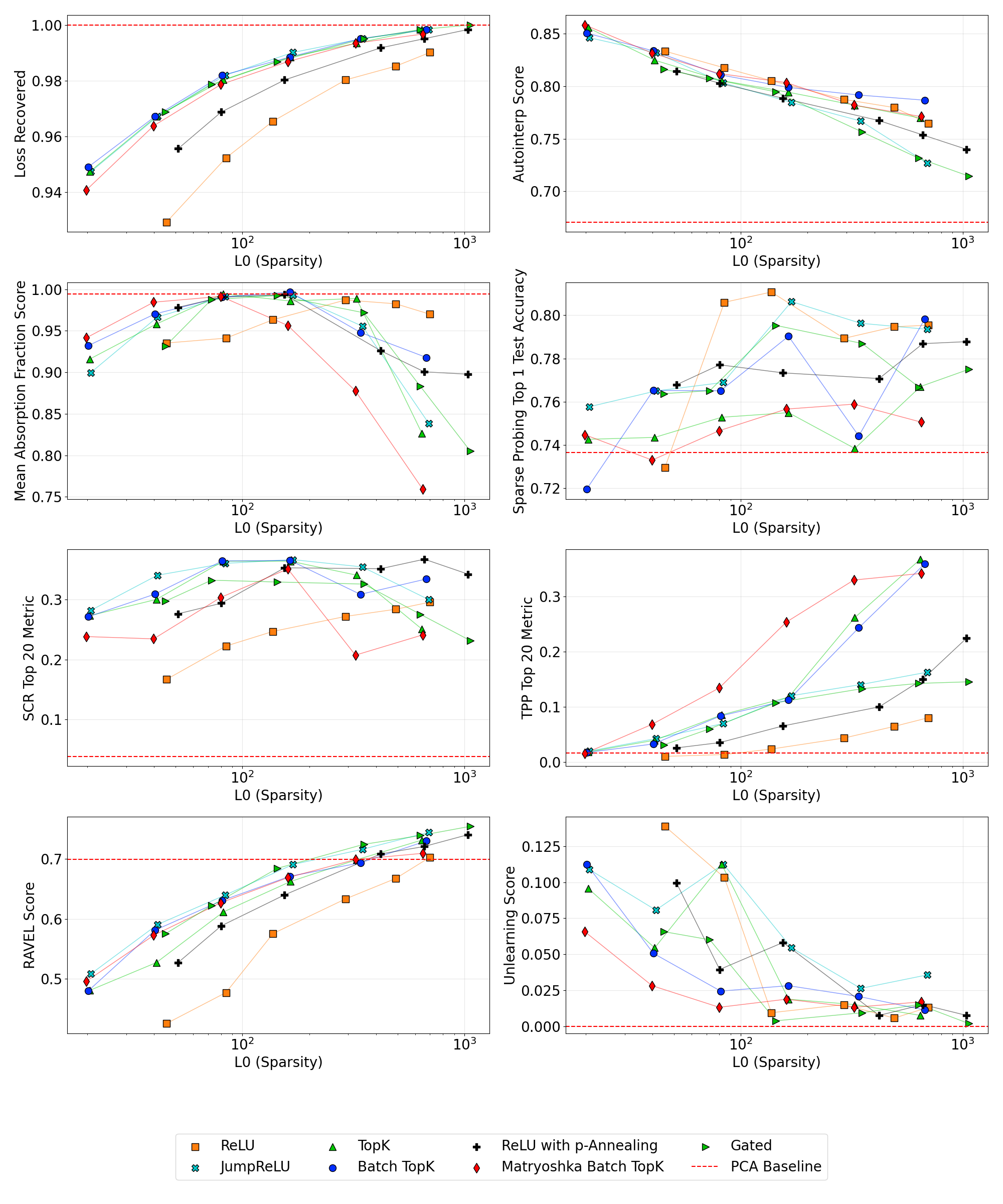
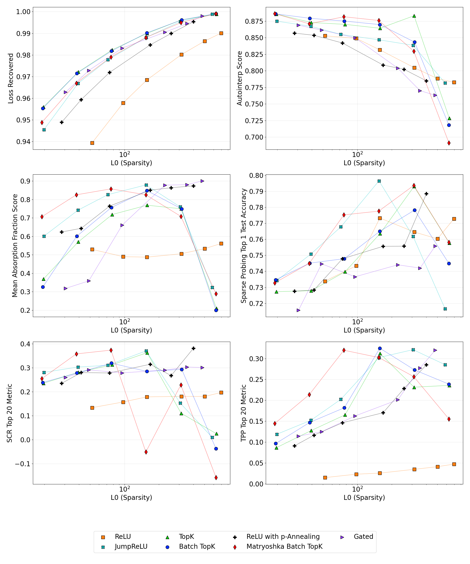
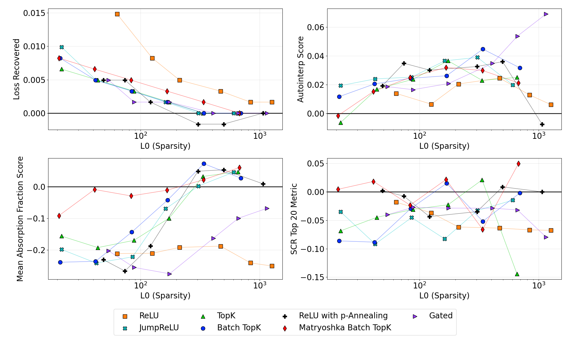
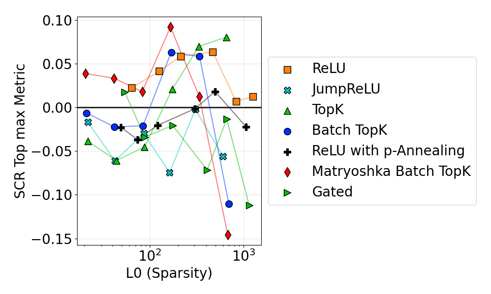
Matryoshka BatchTopK performs best on several concept-detection and disentanglement tests, especially with about 40–200 active latents, although it is not best on reconstruction. Standard ReLU is weaker on five of eight metrics but remains competitive on unlearning and can lead single-latent probing at high activation counts. Rankings depend on the metric and sparsity range; reconstruction rankings alone miss these differences.
4.2 Dictionary Size Scaling Dynamics
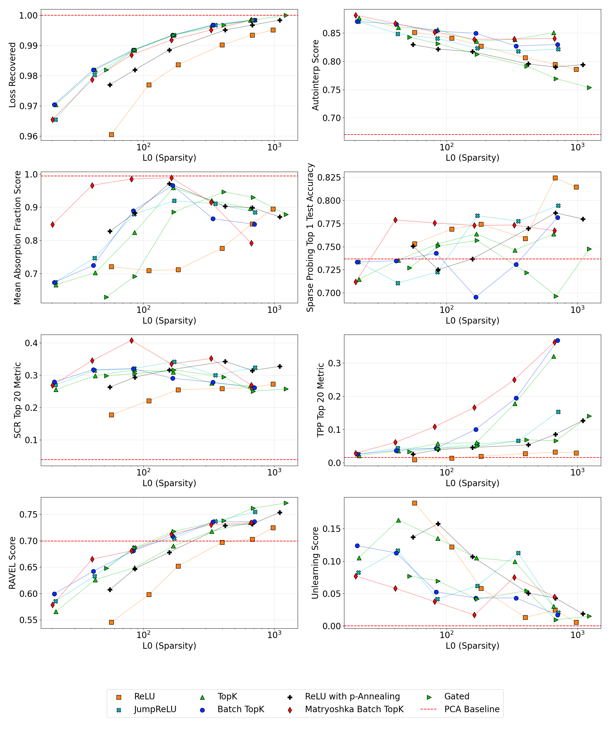
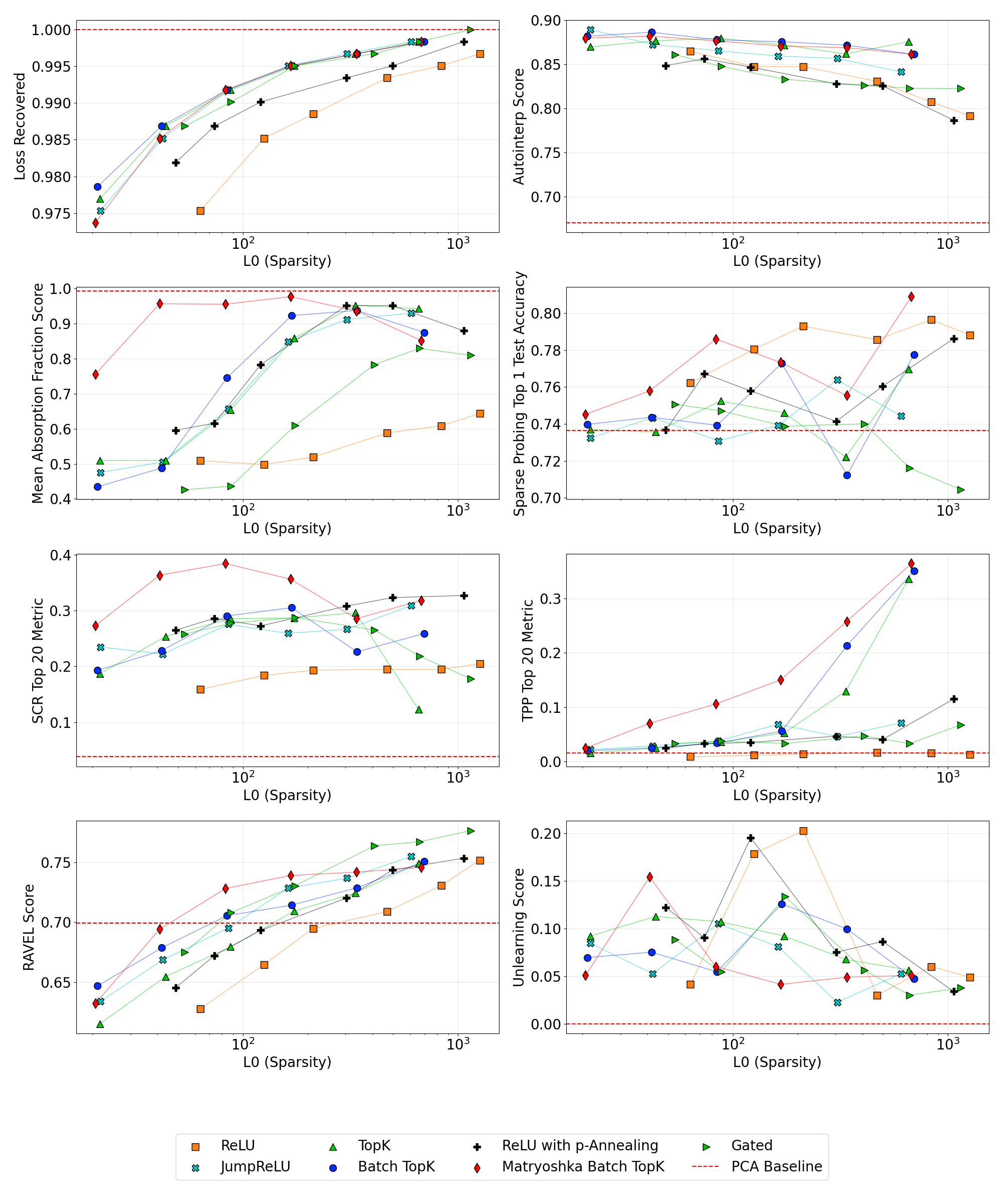
Larger dictionaries generally improve reconstruction and automated feature-description scores. Yet most non-hierarchical architectures become worse at absorption or concept removal as width increases. Matryoshka behaves differently, often improving concept separation. Feature splitting is a proposed explanation, not a demonstrated sole cause. The inverse trend persists across multiple intervention budgets, and the width comparison fixes training data rather than compute.
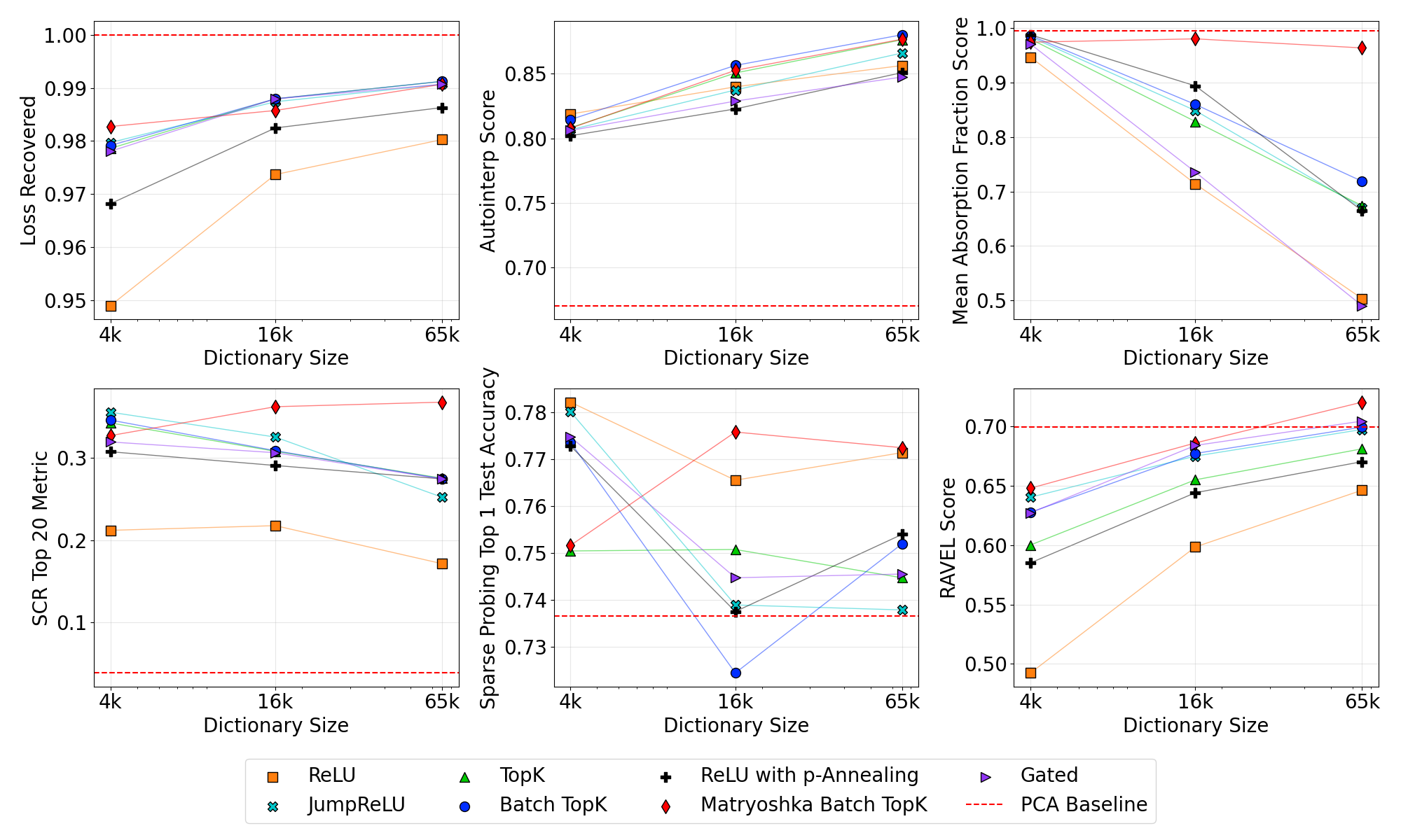
4.3 Task-Dependent Optimal Sparsity
There is no universally best sparsity. Fewer active latents can help feature interpretability, while more can improve reconstruction, RAVEL, and TPP. About 50–150 active latents offers a reasonable compromise in this study; the appropriate choice depends on the intended task.
4.4 Monitoring Training
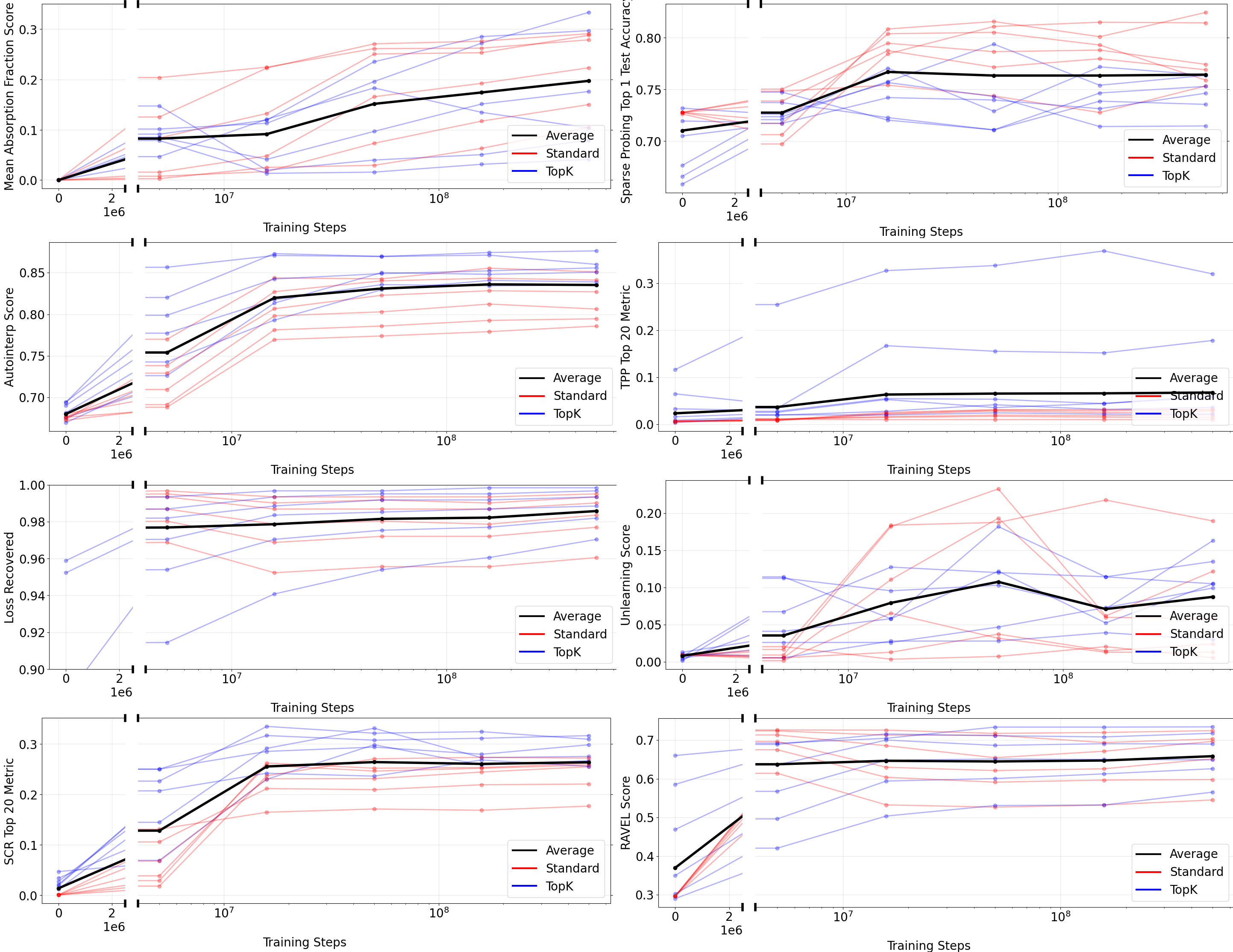
Checkpoint evaluations of 16,000-latent TopK and ReLU SAEs show that many metrics improve quickly within the first 50 million training tokens, then improve more slowly through 500 million. Small metric gains may still correspond to useful qualitative changes, and this does not establish sufficient training budgets for larger dictionaries.
4.5 Model Scale Effects
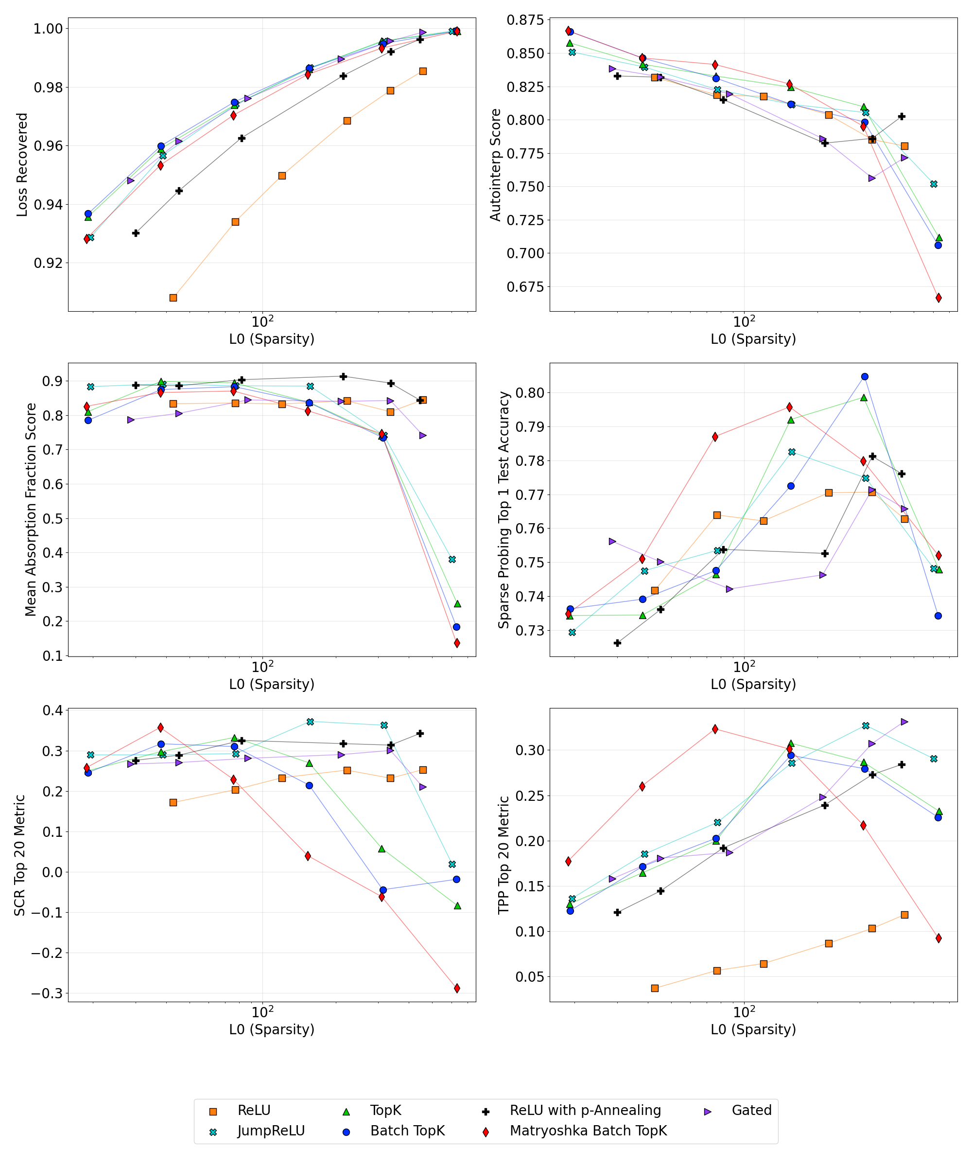
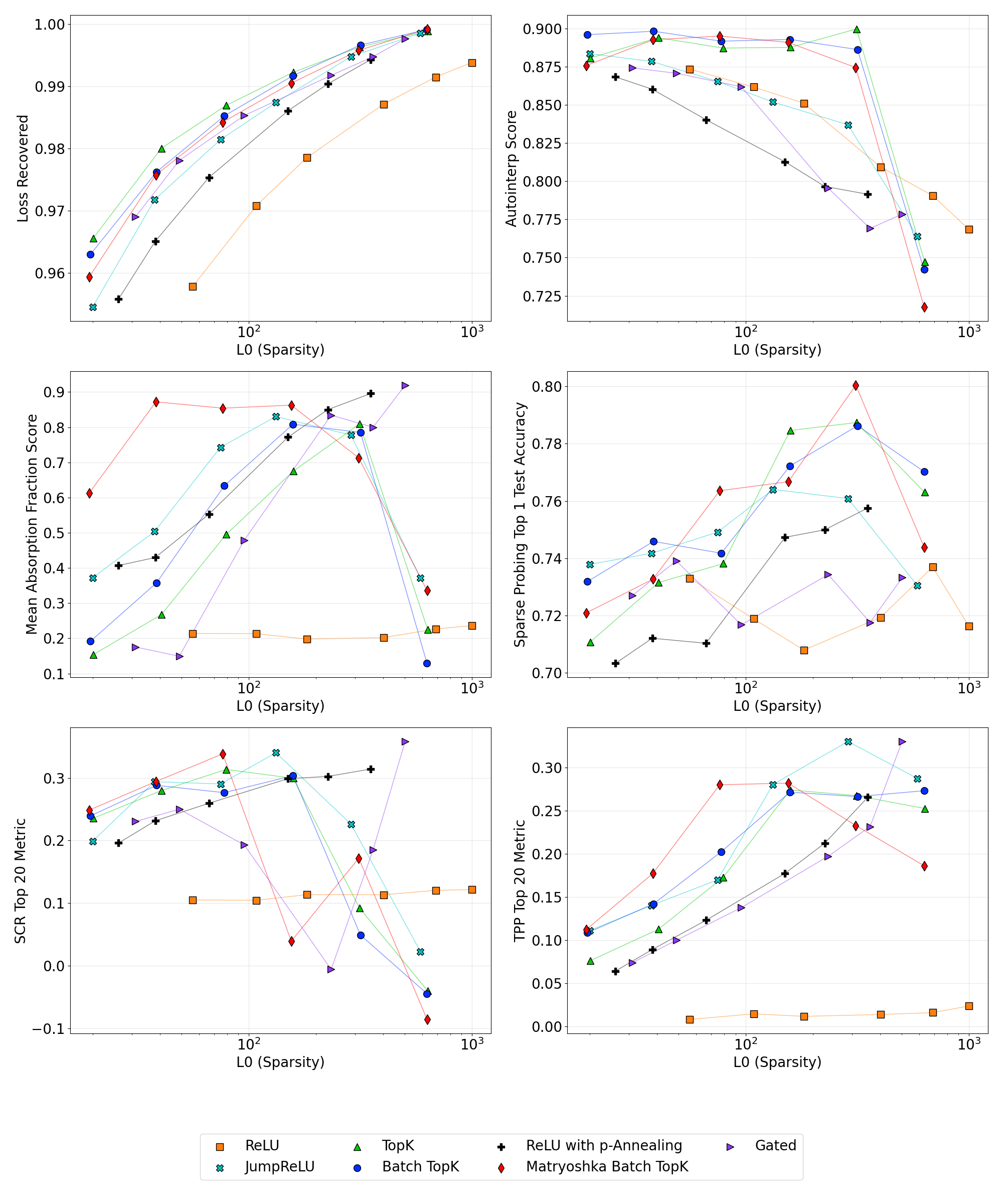
Reconstruction trends transfer more consistently between Pythia-160M and Gemma-2-2B than supervised concept metrics do. Matryoshka’s SCR advantage in Gemma is absent in the smaller Pythia model. The authors suggest that weaker underlying representations of concepts such as spelling or professions can make these evaluations less informative in smaller models.
4.6 Unexpected Findings and Limitations
RAVEL and especially TPP sometimes prefer more than 400 active latents, well above common interpretability settings; SCR does not show the same preference. Sparse probing distinguishes architectures only weakly. Unlearning comparisons are limited because the small base model answers too few questions reliably on most candidate datasets.
5 Limitations
Labeled concepts cover only a small fraction of the features a language model may encode, and some scores are noisy. Automated quantitative tests miss aspects of insight gained through manual analysis. Findings from these models, layers, and training settings need not generalize universally. The metrics have different meanings and scales, so combining them into one overall score would impose arbitrary priorities and hide trade-offs.
6 Conclusion
SAEBench makes it possible to compare reconstruction, explanation quality, and selective feature use together. The main lesson is to evaluate the property an application actually needs: a more accurate or wider SAE is not automatically a better explanatory tool. The authors release the benchmark and SAE suite and propose broader models, modalities, and qualitative evaluations as future work.
Impact Statement
The intended benefit is better tools for understanding and diagnosing model behavior. The authors also acknowledge that interpretability improvements may advance general AI capabilities and carry both benefits and risks.
Acknowledgements
The collaboration received support from MATS, Open Philanthropy, and Lambda compute grants, with additional technical and organizational assistance acknowledged in the source.
Author Contributions
Adam Karvonen and Can Rager co-led the project, experiments, and manuscript. The team contributed metric implementations, training infrastructure, evaluations, and the Neuronpedia results interface; Samuel Marks and Neel Nanda supervised the work.
Appendix A Computational Requirements
For a 16,000-latent SAE on Gemma-2-2B using an NVIDIA RTX 3090 GPU, the benchmark takes about 107 minutes of reusable setup and 65 minutes per SAE. The table separates each evaluation’s setup and recurring costs; larger dictionaries, models, or different hardware change these times.
Appendix B SAE Training Details
Each layer–width–architecture configuration targets six active-latent counts from 20 to 640, though penalty-based methods need not hit the targets exactly. Training data and ordering are held fixed. Activations are normalized during training and the scale is folded into the final weights. Transpose initialization of the decoder helps avoid dead latents; a shuffled activation buffer reduces sequence correlations.
Appendix C Extended Related Work
C.1 SAE Benchmarks
Earlier benchmarks offer complementary evidence: generated feature explanations, downstream loss, sparse probes, sparse ablation effects, board-game ground truth, and task-specific supervised dictionaries. Ground-truth comparisons are often informative but restricted to known features or circuits. SAEBench combines accessible tests while retaining those scope limitations.
Appendix D Further Evaluation Details
All evaluations mask beginning-of-sequence, end-of-sequence, and padding tokens to accommodate SAEs not trained on those special positions.
PCA Baseline Implementation
The PCA baseline is fitted to 200 million activations. All principal components are treated as latents, with a transpose decoder and mean bias. It reconstructs perfectly but is dense, so its scores show what feature discovery gains beyond an invertible change of basis.
Core Evaluation Metrics
Additional diagnostics include reconstruction bias, KL divergence, maximum cosine similarity between latents, and the fraction of high-frequency latents, alongside sparsity and loss recovered.
| Parameter | Value |
| Dataset | OpenWebText |
| Context length | 128 tokens |
| Loss Recovered samples | 3,200 sequences |
| Sparsity evaluation samples | 32,000 sequences |
LLM Scoring / Automated Interpretability
GPT-4o mini generates feature explanations from highly activating and activation-weighted examples. It then classifies a shuffled test set containing ten random, two maximally activating, and two importance-weighted sequences. The detection score measures agreement with observed activation behavior; its validity depends on the explanations, judge, and sampling procedure.
| Parameter | Value |
| Sample size | 1,000 non-dead latents |
| Dataset | The Pile |
| Activation dataset size | 2M tokens |
| Context length | 128 tokens |
| LLM judge | gpt4o-mini |
Sparse Probing
The sparse-probing suite contains 35 binary tasks from five datasets. It uses 4,000 training and 1,000 test examples per task, truncates inputs to 128 tokens, averages non-padding activations, and selects latents by mean difference before fitting logistic regression. GitHub examples omit the first 150 characters to reduce reliance on license headers.
| Dataset | Task Type | Description |
| bias_in_bios | Profession Classification | Predicting professional roles from biographical text |
| Amazon Reviews | Product Classification and Sentiment | Dual tasks: category prediction and sentiment analysis |
| Europarl | Language Identification | Detecting document language |
| GitHub | Programming Language Classification | Identifying coding language from source code |
| AG News | Topic Categorization | Classifying news articles by subject |
RAVEL
RAVEL retains entities and templates that the base model answers accurately, then trains a Multitask Differentiable Binary Mask on 7,000 examples and tests on 3,000. Interventions affect the entity’s final token. Cities and Nobel laureates supply different attribute sets. A jointly trained alignment-search baseline provides a performance reference. Unlike SCR and TPP, this implementation omits the original SAE reconstruction-error residual because including it slightly worsened RAVEL scores.
| Parameter | Value |
| Top entities selected | 500 |
| Top templates selected | 90 |
| MDBM training samples | 7,000 (50% cause, 50% isolation) |
| MDBM test samples | 3,000 |
| MDBM Start Temperature | 1 |
| MDBM End Temperature | |
| MDBM epochs | 2 |
| MDAS epochs | 10 |
| MDBM learning rate | |
| Skyline disentangle score | 0.87 |
Feature Absorption
For each initial letter, a logistic-regression probe on model activations defines a reference direction. Sparse probes identify the main corresponding SAE latents; additional latents count as genuine feature splits when adding them improves F1 by more than 0.03. Absorption is evaluated only on tokens the reference probe classifies correctly.
A case counts when the main latents underrepresent that direction and other sufficiently aligned latents compensate. The score measures the fraction of the represented feature supplied by those compensating latents, allowing partial absorption and several contributors. The preserved equations and table define thresholds precisely. Reported plots use one minus absorption, so larger values are better. The task uses vocabulary tokens containing English letters and an optional leading space, rather than arbitrary semantic hierarchies.
Equations
| Parameter | Value |
| Train/test split | 80/20 |
| -sparse probing max | 10 |
| 0 | |
| SAE dictionary size |
Unlearning
The unlearning sweep varies the maximum retain-set activation frequency, the number of selected latents, and the negative-clamping strength. It evaluates only questions the base model answers correctly under every answer permutation. Among settings retaining more than 99% accuracy on the chosen unrelated MMLU questions, the score selects the best suppression of WMDP-bio answers. This is an operating-point selection on a restricted evaluation set.
| Parameter | Value |
| MMLU Subsets | High School US history,
College Computer Science, High School Geography, Human Aging |
| Retain thresholds | [0.001, 0.01] |
| Number of latents | [10, 20] |
| Negative multipliers | [25, 50, 100, 200] |
| Retain / Forget Dataset size | 1,024 sequences |
| Retain / Forget Sequence length | 1,024 tokens |
Spurious Correlation Removal (SCR)
SCR constructs both perfectly correlated and balanced label combinations from profession–gender or product-category–sentiment datasets. A biased classifier is trained on the correlated data. Probe attribution selects latents associated with the unwanted signal, which are zero-ablated while retaining the original reconstruction residual. Improvement on balanced data is normalized between the biased classifier and a classifier trained directly on the desired concept.
Equations
Targeted Probe Perturbation (TPP)
TPP trains a binary probe per class and selects latents with positive attribution to that class. It compares the effect of each ablation on its matching probe against effects on the other probes. A high score indicates selective changes within that model’s probe system. The appendix lists the profession and product classes used, along with the SCR class pairs.
Equation
Appendix E Baseline Comparison: SAEs on Randomly Initialized vs. Fully Trained Models
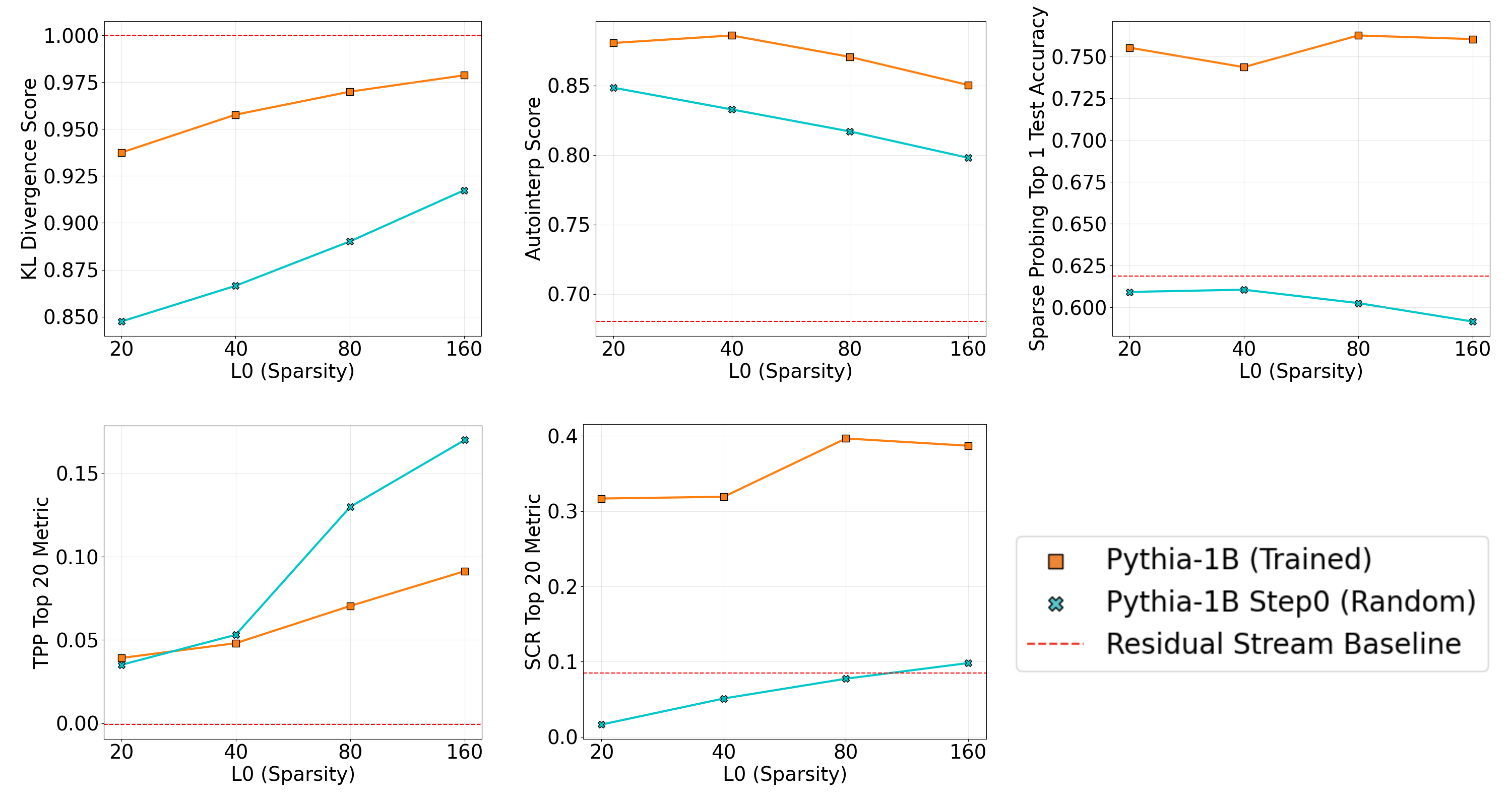
A control compares 16,000-latent TopK SAEs trained for 100 million tokens on layer 10 of either trained or randomly initialized Pythia-1B. It examines reconstruction, sparse probing, automated interpretation, SCR, and TPP to check which metrics distinguish learned model structure from random representations.
Limitations and Contextual Considerations:
These metrics were designed mainly to compare SAEs on the same model. Random models lack the capabilities required by some tasks, and their probes start from lower accuracy: full-residual probing reaches 84% here versus 94% for the trained model. Relative intervention scores should therefore not be treated as directly comparable measures of understanding across the two models.
Supervised Metrics:
SAEs on the trained model perform substantially better on sparse probing and SCR. On the random model, SAE probes approach or underperform probes on the raw residual stream.
Automated Interpretability:
Automated interpretation scores are only slightly higher on the trained model, although both SAE sets beat direct residual-channel readings. This detection-style test differs from alternative fuzzing tests. High scores on random-model features limit what automated interpretation alone can establish.
KL Divergence:
Because next-token loss recovery is uninformative for a random model, the comparison uses KL divergence normalized against zero ablation. Trained-model SAEs recover more of the original output distribution relative to that baseline, even though their absolute KL divergence is larger.
Equation
Targeted Probe Perturbation (TPP):
Random-model SAEs score higher on TPP in this comparison. The authors caution that this relative probe-accuracy metric has different baselines across the two models, so the result does not imply that random-model features provide better practical interpretation.
Appendix F Additional Dictionary Scaling Analysis
The expanded plots show width scaling at each sparsity, rather than averaging over 40–200 active latents. They make operating-point dependence visible while making direct architecture comparisons less compact.
Appendix G Training Dynamics
The checkpoint plots retain full training trajectories for TopK and ReLU SAEs, showing which metrics saturate early and which continue improving.
Appendix H Intervention Set Size Analysis
Ablation tests sweep 5–500 latents, while sparse probes use one, two, or five. Architecture rankings are broadly similar for intervention budgets of 5–50 but can change at 500. The main choice of 20 balances concept coverage against the feasibility of manual inspection. Allowing several probe latents also increases the SAE advantage over PCA.
Appendix I Gemma-Scope Evaluation Results
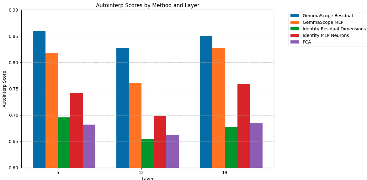
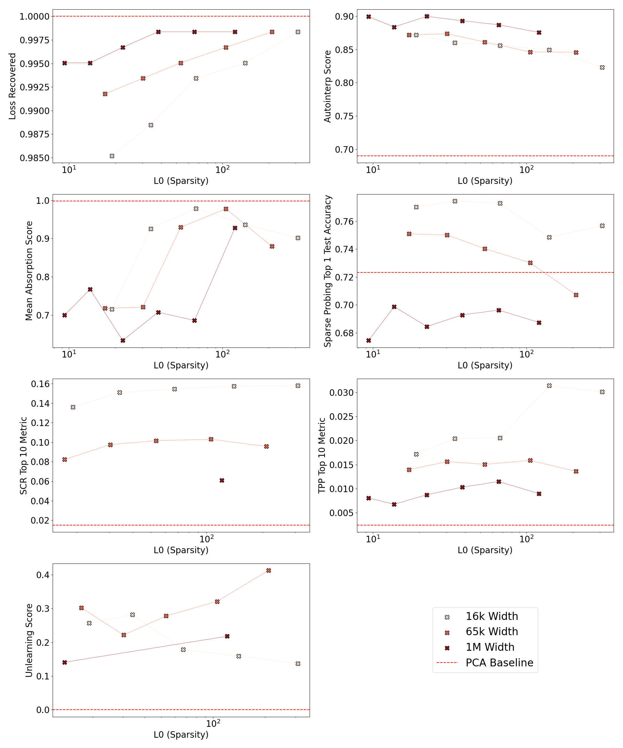
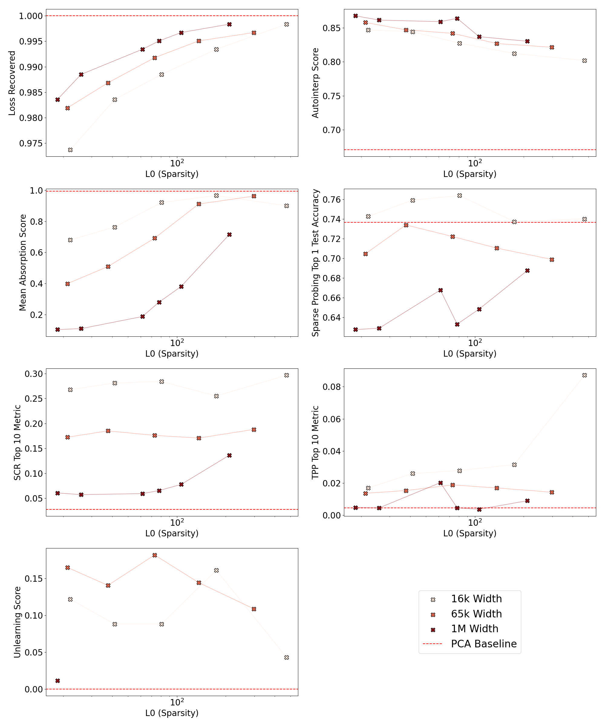
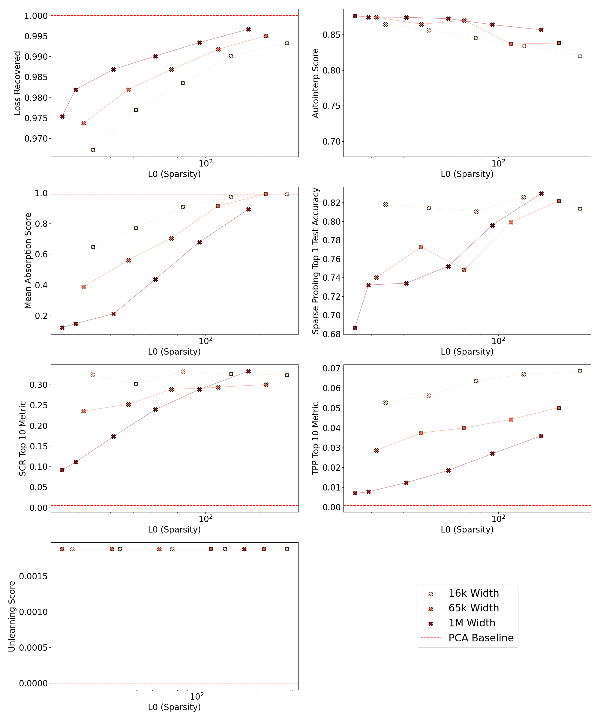
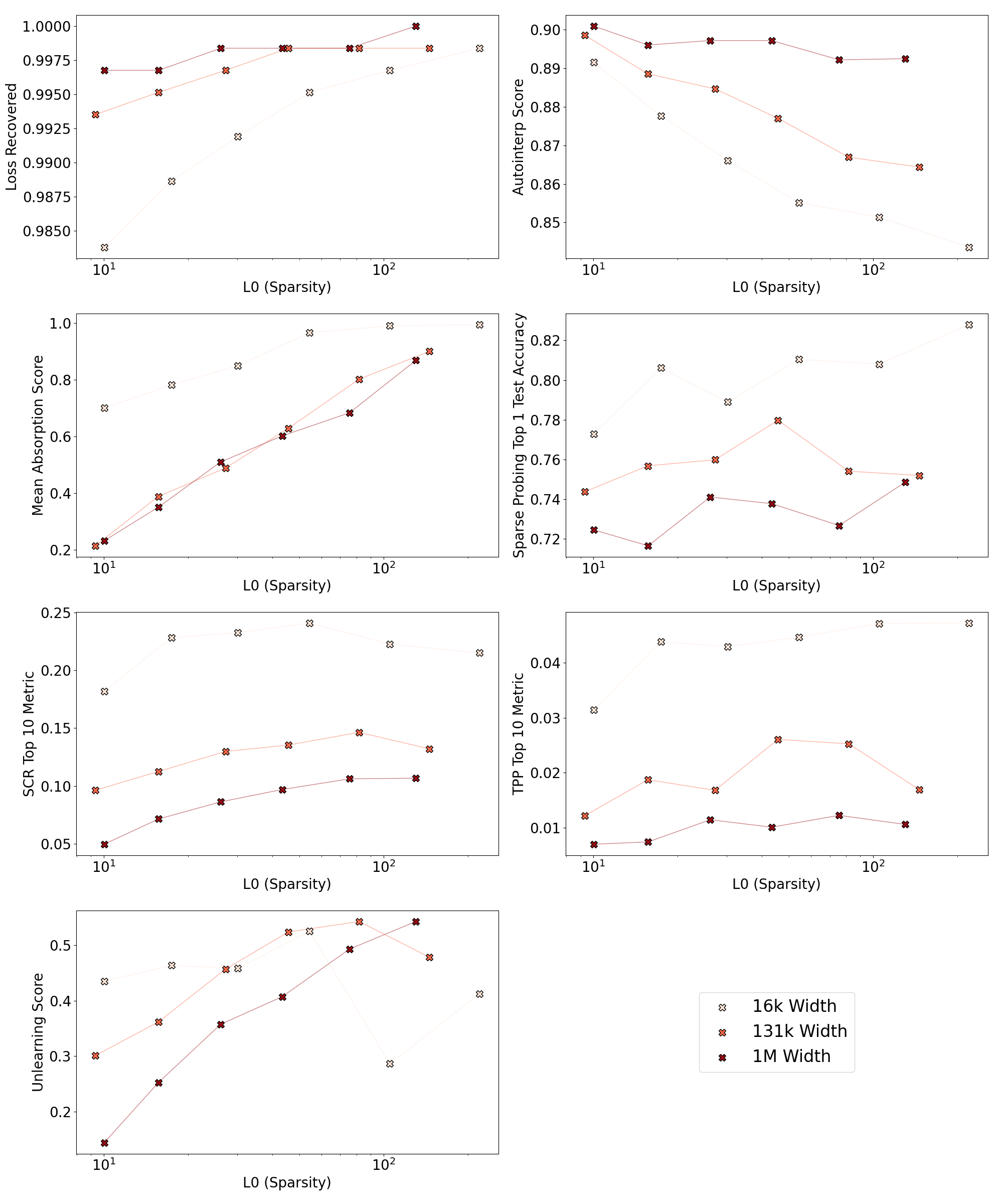
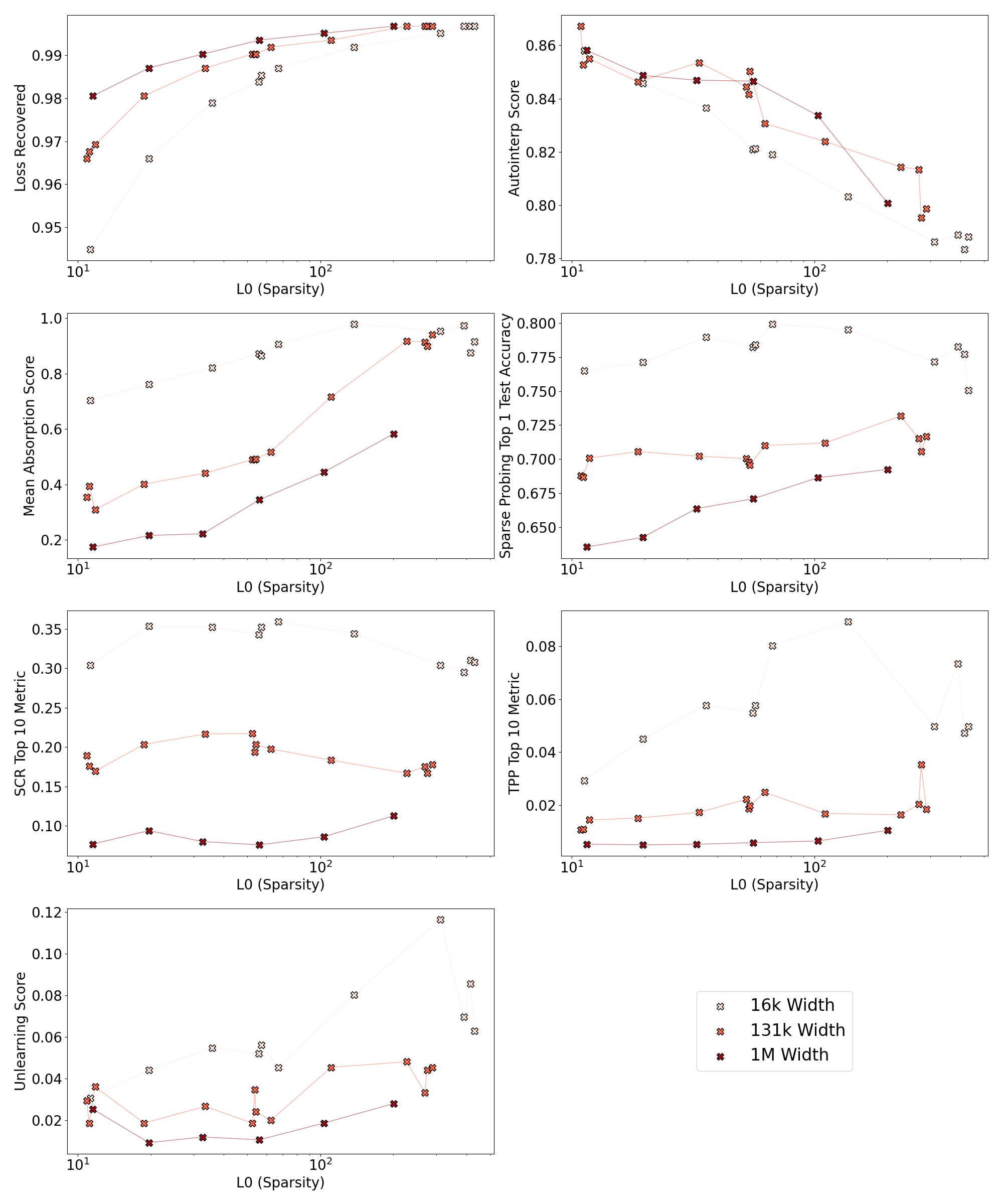
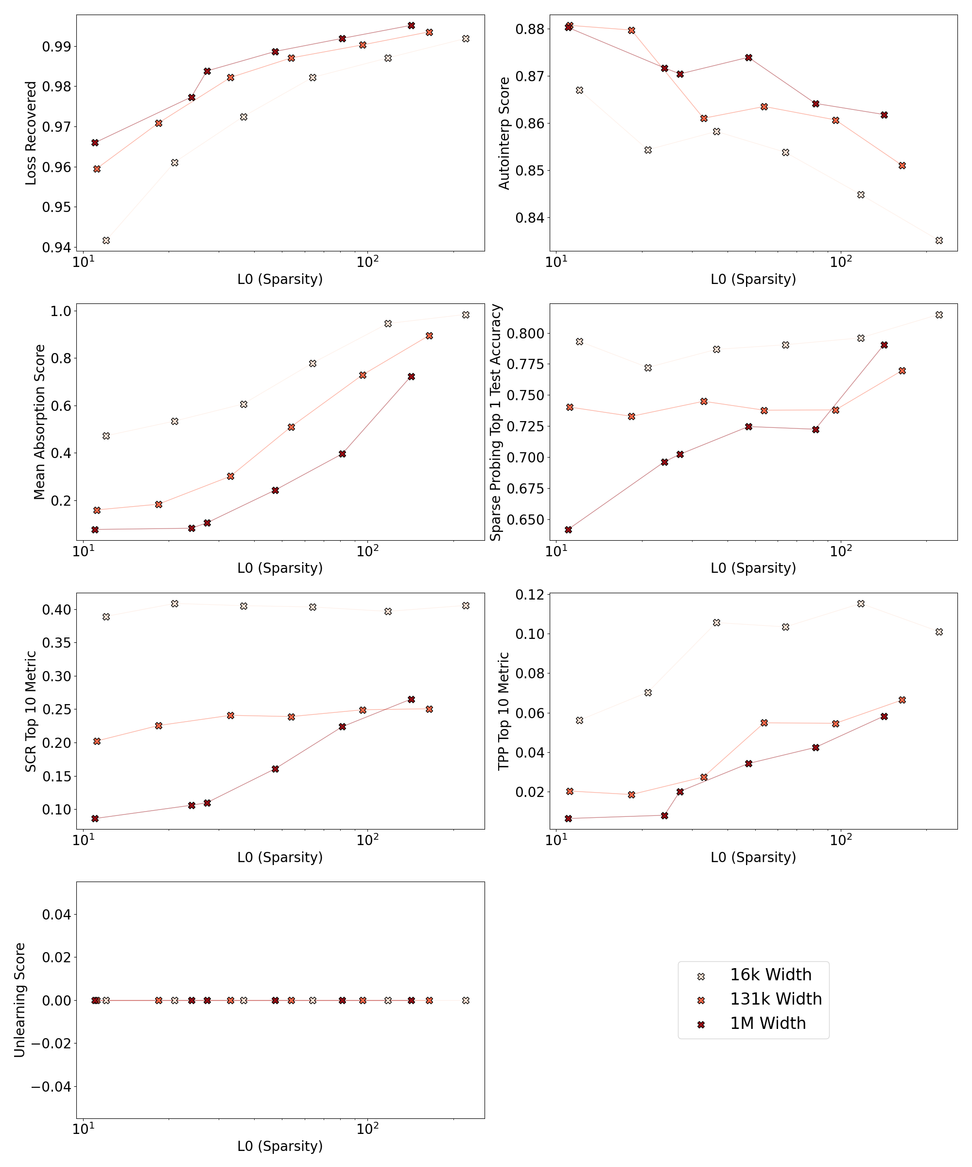
Gemma Scope extends evaluation across three layers each of Gemma-2-2B and Gemma-2-9B, with widths up to one million latents. Results vary strongly by layer: later layers perform poorly on this unlearning test, while sparse probing improves. Wider dictionaries generally improve reconstruction and automated interpretation but worsen absorption, SCR, and TPP, echoing the non-hierarchical scaling trade-offs in the main suite.
Appendix J Further SAE Bench Evaluation Results
The final figures retain the complete per-metric comparisons across dictionary widths and the two main base models. They show how the central Gemma results depend on sparsity, architecture, and model capability.