At a glance
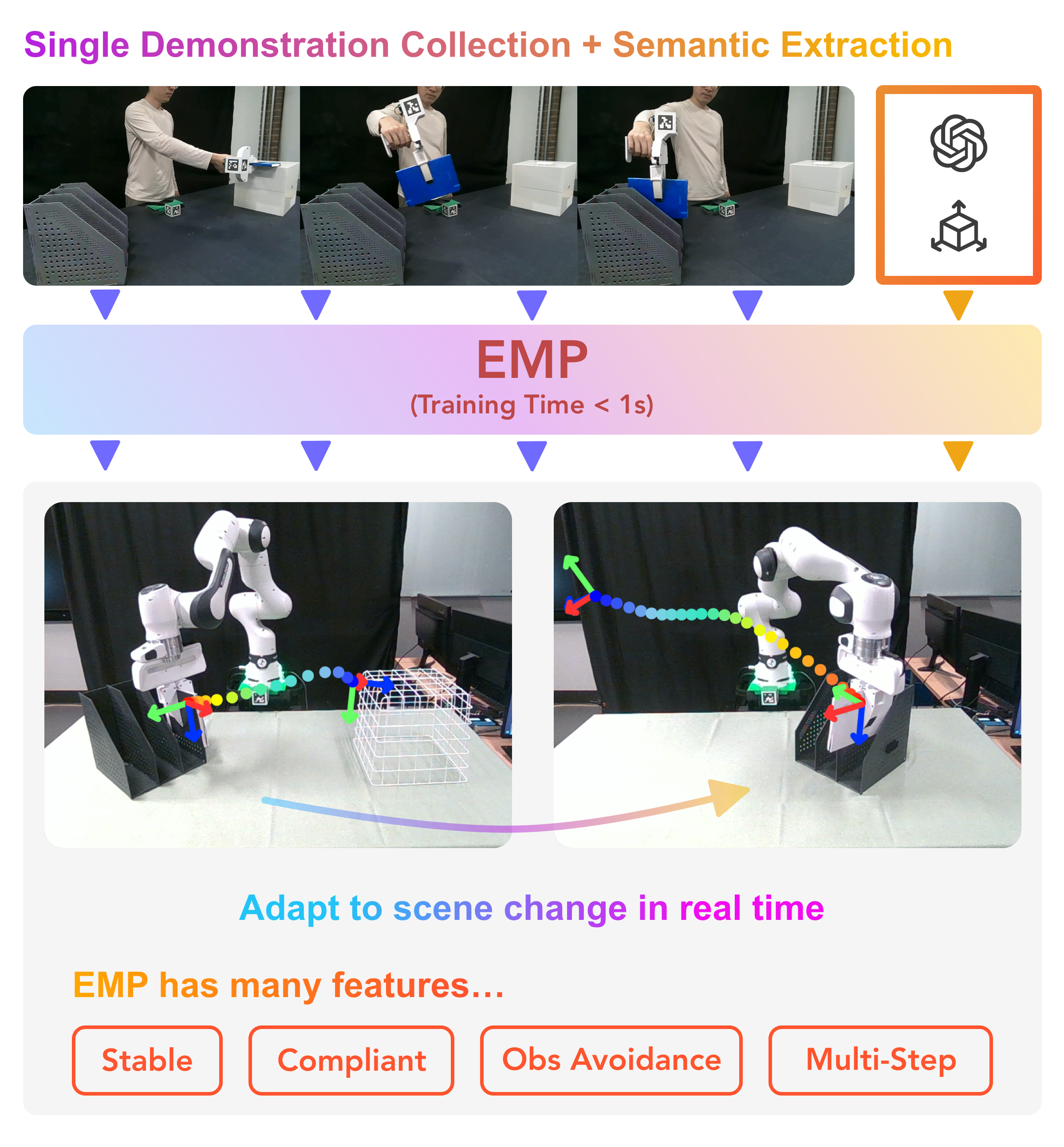
EMP adapts a full-pose robot motion learned from one demonstration when relevant objects move. It deforms the policy’s Gaussian geometry, including orientation in quaternion tangent coordinates, and rapidly refits stable local dynamics. A visual pipeline identifies and tracks task keyposes. Real-robot tests show stronger generalization than rigidly transforming a fixed policy, with limitations from tracking, segmentation, and robot reachability.
I INTRODUCTION
A stable motion can still become inappropriate when the scene changes. EMP extends Elastic-DS from position trajectories to full end-effector pose and replaces slow potential fitting with a convex formulation. The reported update rate is about 30 Hz. It assumes known object meshes and usable object tracking, and integrates optional obstacle avoidance and multistep segmentation. [3]
II RELATED WORK
The paper contrasts collecting more demonstrations with constraining and adapting the policy itself. Stable DS methods help recover from unfamiliar states but typically retain a fixed task geometry. EMP focuses on changing that geometry efficiently, using few demonstrations and explicit task keyposes rather than a large end-to-end visual policy.
III BACKGROUND
EMP builds on separate but coordinated position and orientation dynamical systems, each using a mixture of local models.
III-A SE(3) Linear Parameter Varying Dynamical System
Position uses an LPV-DS in Euclidean space. Orientation uses a quaternion dynamical system represented in a tangent space. The combined construction approximates full rigid-body pose as position plus rotation.
III-A 1 LPV-DS Formulation
A Gaussian mixture supplies state-dependent weights for linear systems sharing one attractor. A positive-definite quadratic Lyapunov function and matrix inequalities constrain every component to decrease the same potential. The mixture then inherits the corresponding convergence property for the fixed policy. Fitting minimizes demonstrated velocity error subject to those constraints.
Equations 1–3
| (1) |
| (2) |
| (3) |
III-A 2 Quaternion Dynamical System
Orientations are mapped relative to the target quaternion with the Riemannian logarithm. Mixture-weighted linear maps predict the next desired tangent-space orientation, and a semidefinite program fits them under the stated stability constraints. This discrete orientation update differs from the continuous position-velocity output.
Equations 4–5
| (4) |
| (5) | ||||
III-A 3 Stable SE3-LPVDS Policy
The two policies produce desired linear and angular motion. Orientation prediction requires parallel transport and an exponential map to recover a unit quaternion, followed by conversion to an angular command. The appendix retains these formulas.
Equation 6
| (6) |
IV ELASTIC MOTION POLICY
Adaptation changes the geometric parameters describing the demonstration, then refits the motion field. Relevant object poses supply endpoint and approach constraints.
IV-A SE3 LPV-DS Policy Morphing
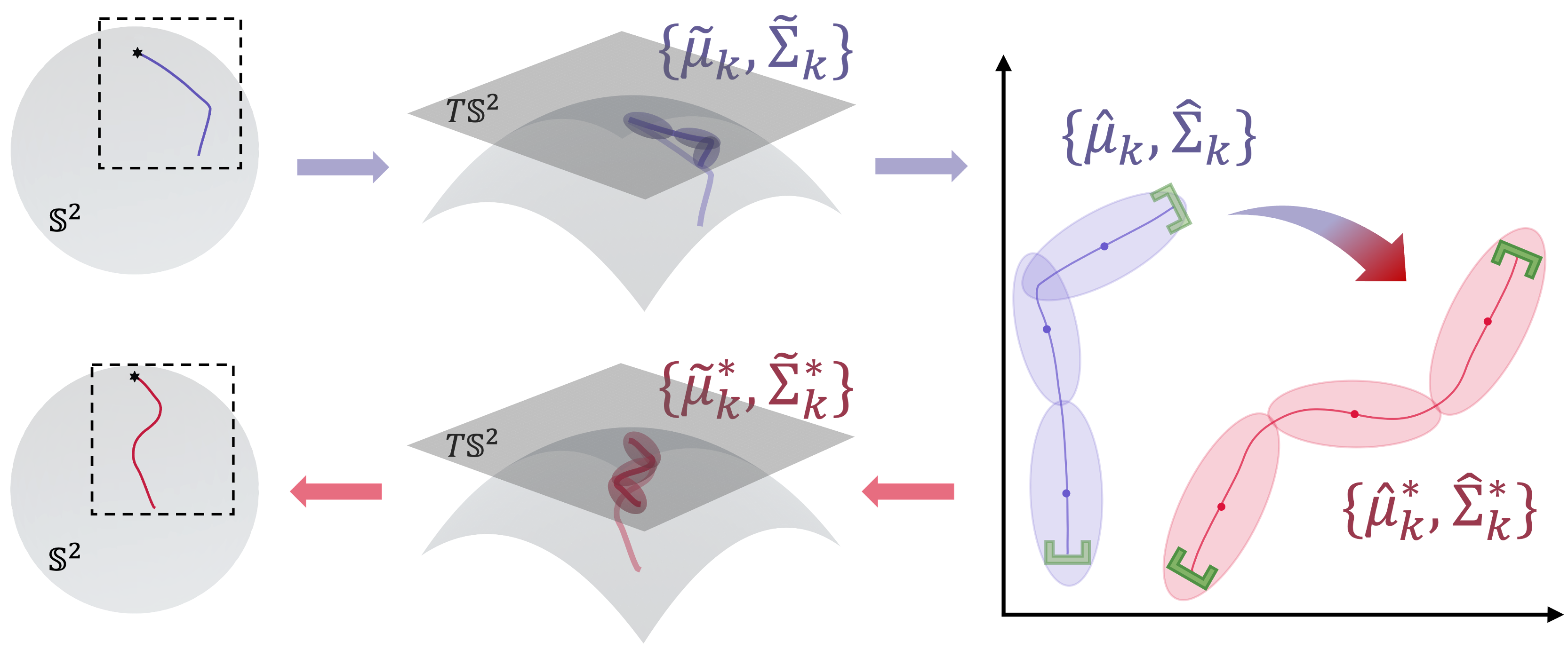
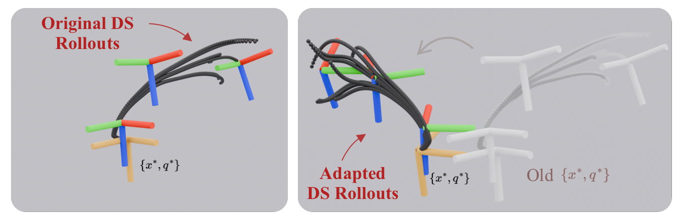
Neighboring Gaussians define intermediate joints along the demonstrated motion. Laplacian editing moves these joints to satisfy new endpoint transformations while approximately retaining their local relationships. The changed means and covariances define a new geometry for policy fitting.
For orientation, the method constructs a three-dimensional basis for the tangent hyperplane embedded in four-dimensional quaternion coordinates. Means and covariances are reduced to those coordinates, edited, and mapped back. The construction uses different bases for the attractor-centered means and mean-centered covariances. Figures 2 and 3 illustrate orientation and full-pose adaptation.
Equations 7–16
| (7) |
| (8) |
| (9) | ||||
| (10) |
| (11) |
| (12) |
| (13) |
| (14) |
| (15) |
| (16) |
IV-B Real-Time Convex Lyapunov Function Optimization
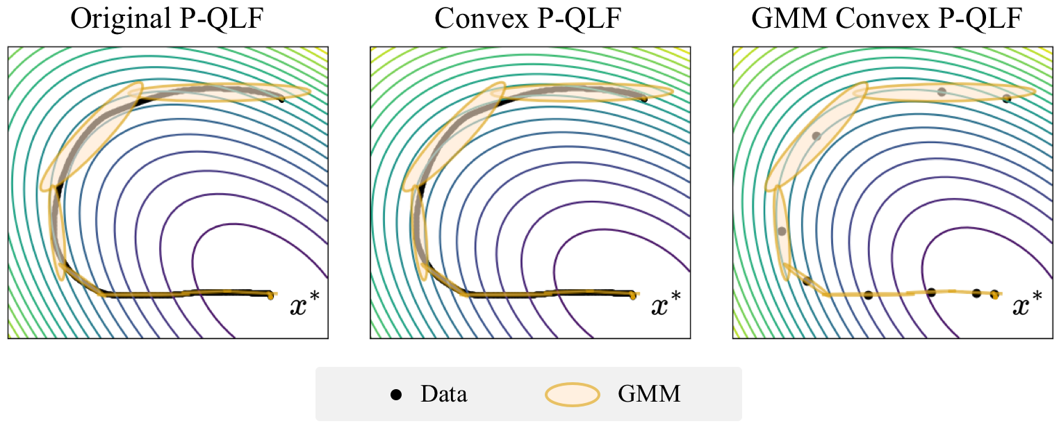
The quadratic potential matrix is fitted with a convex sum of ReLU penalties on positive Lyapunov derivatives, subject to a positive-definiteness constraint. This is a surrogate for reducing derivative violations, not a literal count of them. Fitting subsequent local dynamics still supplies the policy’s matrix stability constraints.
Replacing all demonstrated samples with Gaussian mean positions and velocities makes optimization faster, at the cost of discarding some local detail. The measured derivative-violation rate reflects that tradeoff. The fixed-policy convergence argument should not be read as a separate guarantee for arbitrary rapid changes of targets or policy parameters.
Equations 17–18
| (17) |
| (18) |
V EMP IMITATION LEARNING PIPELINE
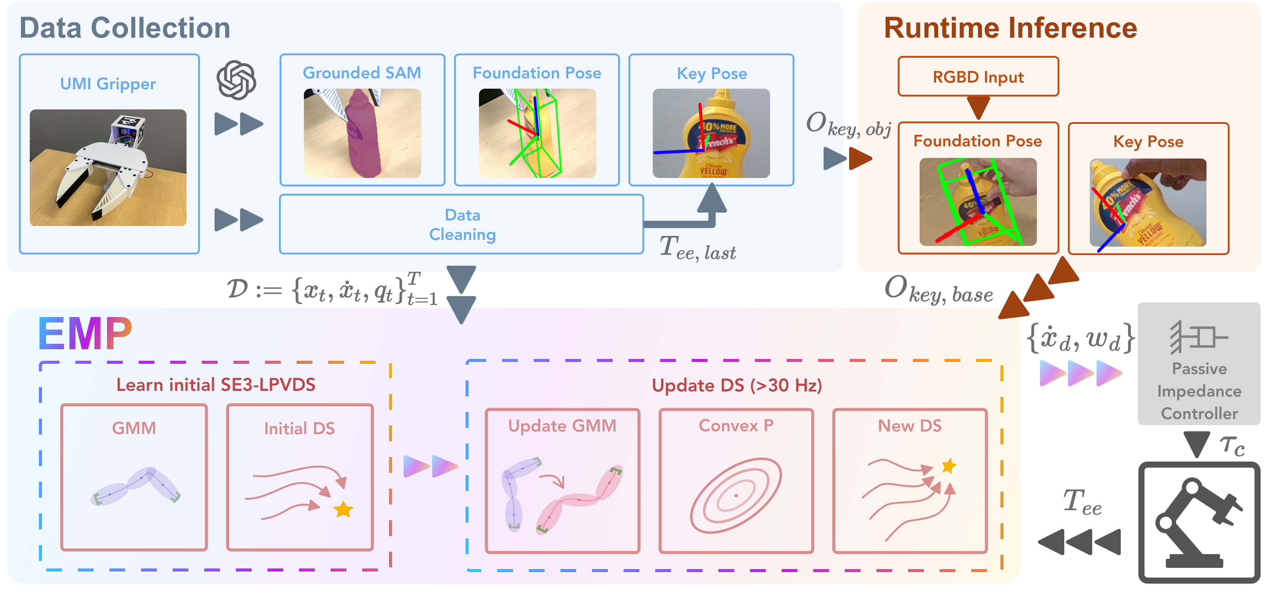
The pipeline collects a demonstration, identifies task-relevant object keyposes, optionally segments the task, and adapts the learned policy during execution.
V-A Data Processing
Demonstration processing produces base-frame end-effector trajectories, gripper states, and object-relative task constraints.
V-A 1 Demonstration Data Collection
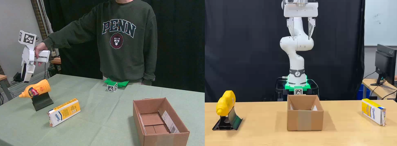
A modified UMI gripper carries several AprilTags for external RGB-D tracking, while a contact sensor records binary gripper state. A reference tag cube defines a consistent robot-base frame during both demonstration and execution. This supports demonstration collection without moving the robot itself.
V-A 2 Keypose/Attractor Extraction
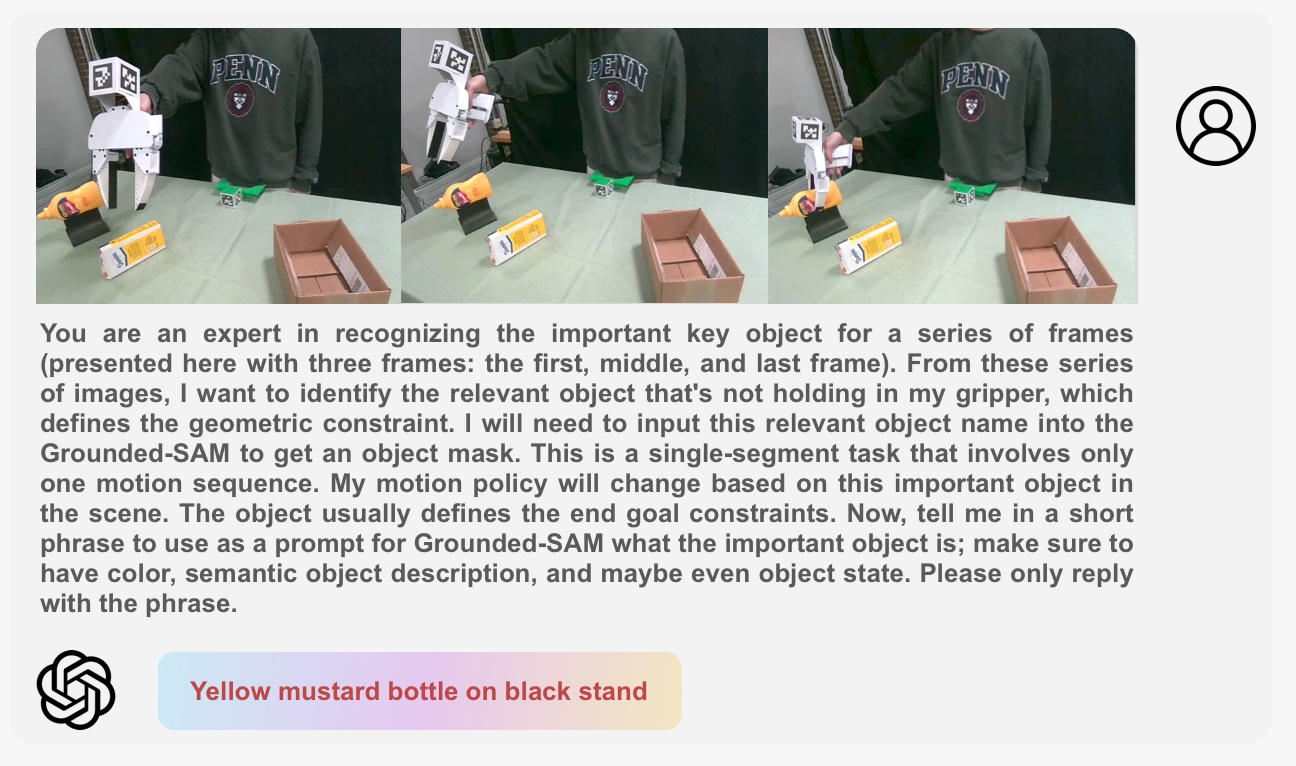
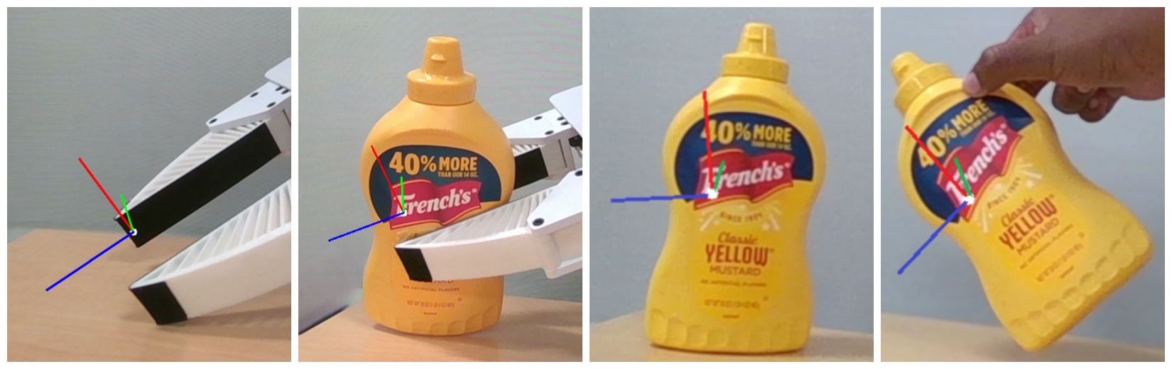
GPT-4o identifies the relevant object from sampled video frames. Grounded SAM produces its mask, and FoundationPose estimates and tracks its pose using the available object mesh. The demonstrated final end-effector pose is stored relative to that object as a keypose; changing object pose updates the task constraint. The original prompt and response appear in the appendix.
V-A 3 Multi-Step Trajectory Decomposition
UVD divides long demonstrations into goal-directed segments. Each segment receives its own policy and object-relative keypose. A one-hot switch activates the next policy after the current attractor is reached. Segmentation errors therefore propagate into the chosen subgoals and can cause task failure.
V-B Runtime Policy Inference
Tracked object poses continuously update geometric constraints, which drive policy deformation and refitting. A passive impedance controller converts the desired velocities to joint torques. Subtask completion triggers policy switching and gripper changes.
VI EVALUATION
Evaluation separates the potential-fitting speed/violation tradeoff from complete robot-task performance.
VI-A Convex Lyapunov Function Evaluation
On thirty LASA handwriting motions, the study compares the prior nonconvex potential fit with full-data and Gaussian-informed convex fits. Single-demonstration trials are repeated ten times per motion, with a further comparison using all seven demonstrations. The Gaussian-informed version approaches a fiftyfold fitting-time improvement in the reported larger-data setting, while its derivative-violation rate can increase. Table I preserves the exact timings and violation percentages.
| LASA Dataset | Methods | Computation Time (s) | Violation Percentage |
|---|---|---|---|
| Single Trajectory | Baseline P-QLF | 0.332 | 14.0% |
| Convex P-QLF | 0.038 | 11.1% | |
| GMM P-QLF | 0.007 | 15.1% | |
| All Trajectory | Baseline P-QLF | 2.62 | 14.9% |
| Convex P-QLF | 0.24 | 12.3% | |
| GMM P-QLF | 0.09 | 15.4% |
| Methods | Book Placing | Cube Pouring | Pick-and-Place | |
|---|---|---|---|---|
| ID | SE(3)-LPVDS | 10/10 | 10/10 | 8/10 |
| EMP (Ours) | 10/10 | 10/10 | 7/10 | |
| OOD | SE(3)-LPVDS | 4/10 | 4/10 | 1/10 |
| EMP (Ours) | 8/10 | 9/10 | 7/10 |
VI-B Real Robot Tasks Evaluation
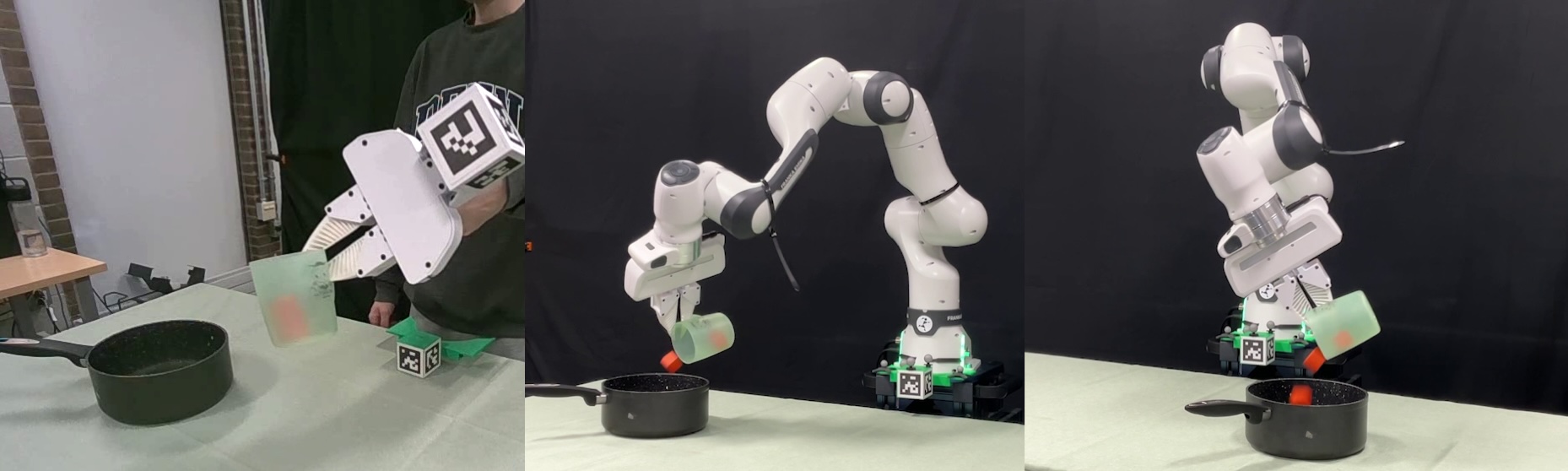
A Franka Research 3 performs book placing, cube pouring, and multistep pick-and-place from one demonstration per task. The baseline rigidly transforms an object-centric SE(3)-LPVDS. Ten trials per task and setting compare demonstrated configurations with more varied object placements. Table II reports success rates; the small trial counts should accompany any comparison.
VI-B 1 Book Placing
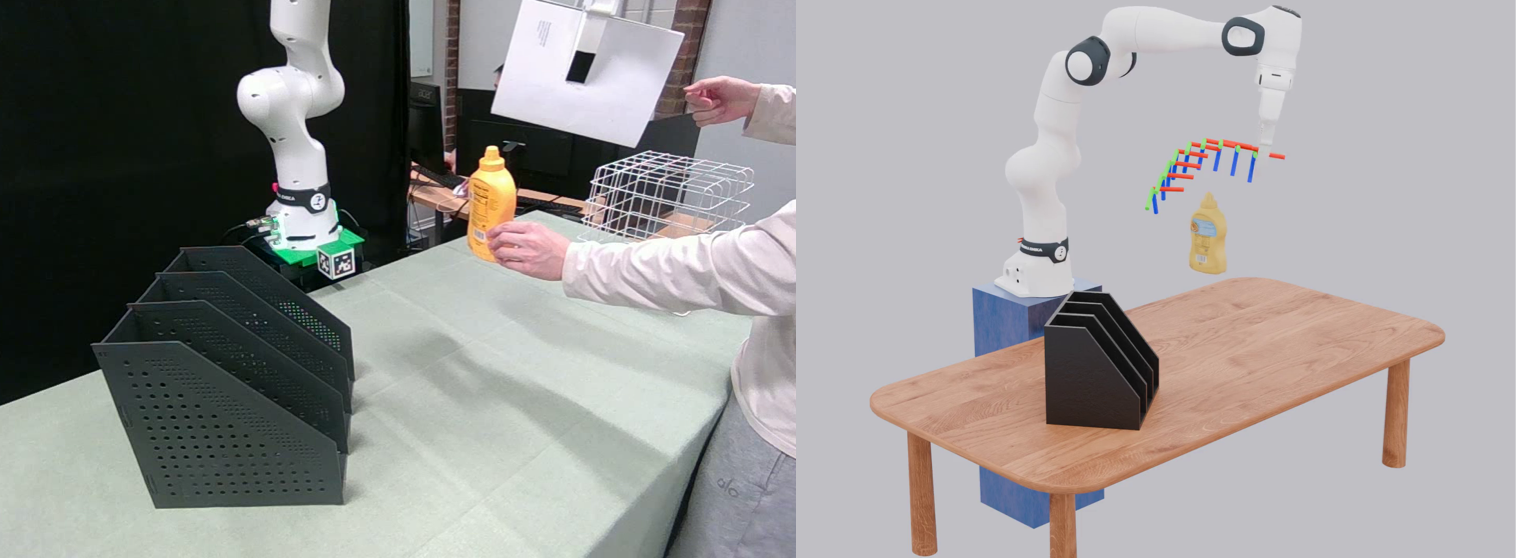
Book placing requires both a correct approach through the rack opening and the final insertion pose. Both methods succeed in the demonstrated setup. Changing the rack pose exposes failures of a rigid whole-policy transformation, whereas EMP can preserve the approach and placement constraints through deformation.
VI-B 2 Cube Pouring
Pouring requires an arched path, wrist rotation, and an upright starting cup. Both methods succeed in the demonstrated setup, but the fixed-policy baseline fails in more than half of the varied trials. EMP better retains the required motion shape, though one case fails at a difficult pouring angle. Task-space adaptation can still generate a path outside the robot’s reach or joint limits.
VI-B 3 Multi-Step Pick-and-Place Task
Repeated pick-and-place uses UVD with γ = 0.003 to obtain sequential subgoals. Errors in segmentation or grasping reduce performance for both methods. Cutting a placing segment too early, for example, puts its attractor outside the box; convergence to that attractor then fails the actual task.
VI-C Case Study: Book Placing with Obstacle Avoidance
A book-placing case study adds a mustard bottle modeled as a sphere of diameter 0.18 m. A standard velocity-field modulation changes the motion in the obstacle-normal and tangent directions. This illustrates compatibility with obstacle avoidance; it is a separate geometric layer and a qualitative example rather than a broad safety benchmark.
VII CONCLUSIONS & DISCUSSIONS
EMP combines fast full-pose deformation with constrained dynamics fitting and shows useful one-shot adaptation. Its dependencies include accurate tracking, object meshes, reliable task segmentation, and feasible robot configurations. A single tangent-space approximation can distort quaternion geometry; richer manifold formulations and potentials are proposed for more complex motions. Multiple demonstrations are discussed as an extension, rather than the main evaluated setting.
-A Quaternion-DS Formulas
The predicted orientation displacement is transported from the attractor tangent space to the current orientation, mapped back to the quaternion manifold, and converted to an angular command using the known time interval. Equations (19)–(21) retain the exact operations.
Equations 19–21
| (19) |
| (20) |
| (21) |
-B GPT Prompt for Semantic Object Extraction
The preserved example gives GPT-4o demonstration frames and asks it to identify the task-relevant object. Its text response becomes the prompt for the segmentation model. This is the object-selection component of the pipeline, rather than an action-generation policy.