Overview
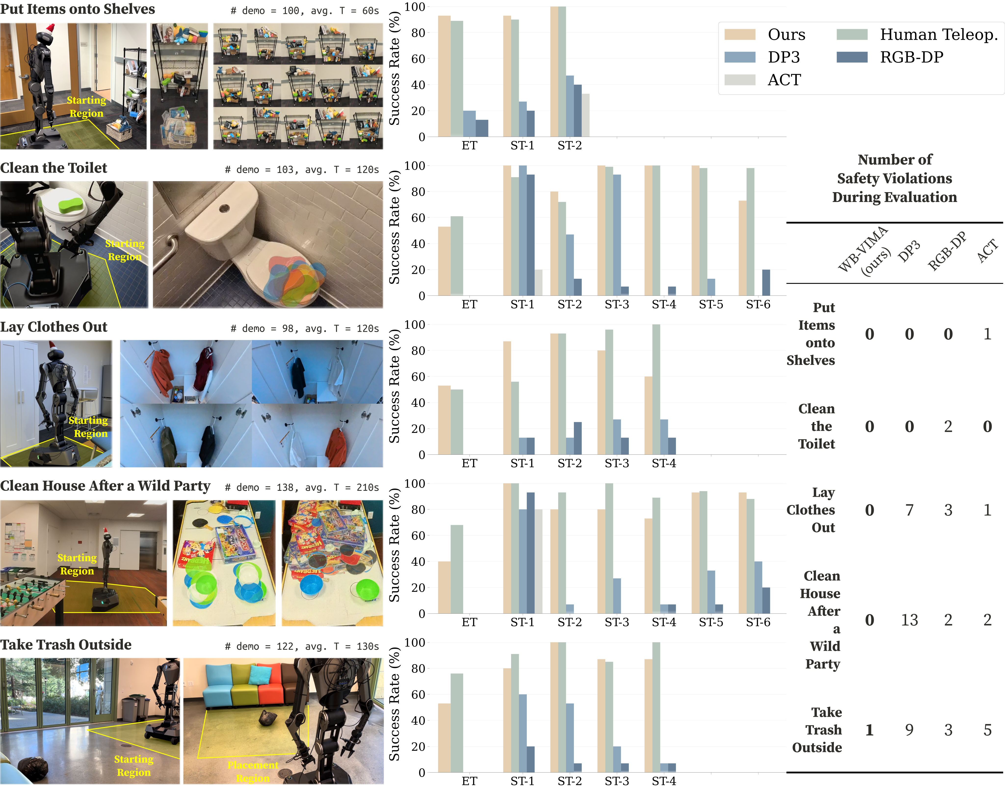
Figure 1 shows the five evaluated household activities and the body capabilities they emphasize: bimanual coordination, navigation, and reachability.
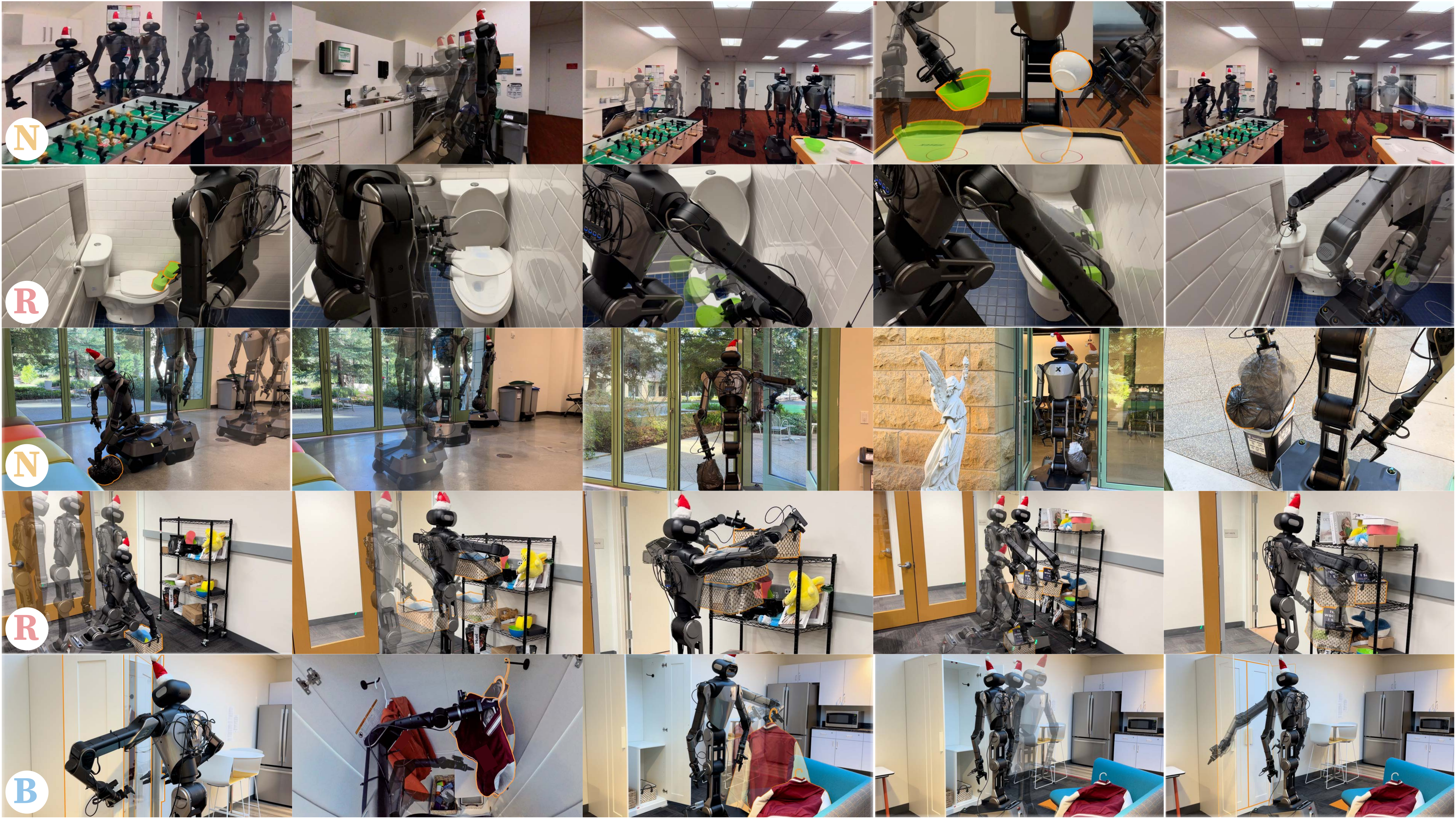
At a glance
BEHAVIOR Robot Suite combines the Galaxea R1 mobile dual-arm robot, the low-cost JoyLo teleoperation interface, and WB-VIMA, a policy that predicts base, torso, and arm actions in sequence. Demonstrations cover five household activities lasting roughly one to three and a half minutes. The paper reports 88% average sub-task success and about 58% average full-task success, with 93% on the best task. These are distinct metrics: failed sub-tasks can be reset before evaluating later sub-tasks. The work demonstrates coordinated whole-body imitation in the tested environments, while broad scene transfer and general household autonomy remain open.
1 Introduction
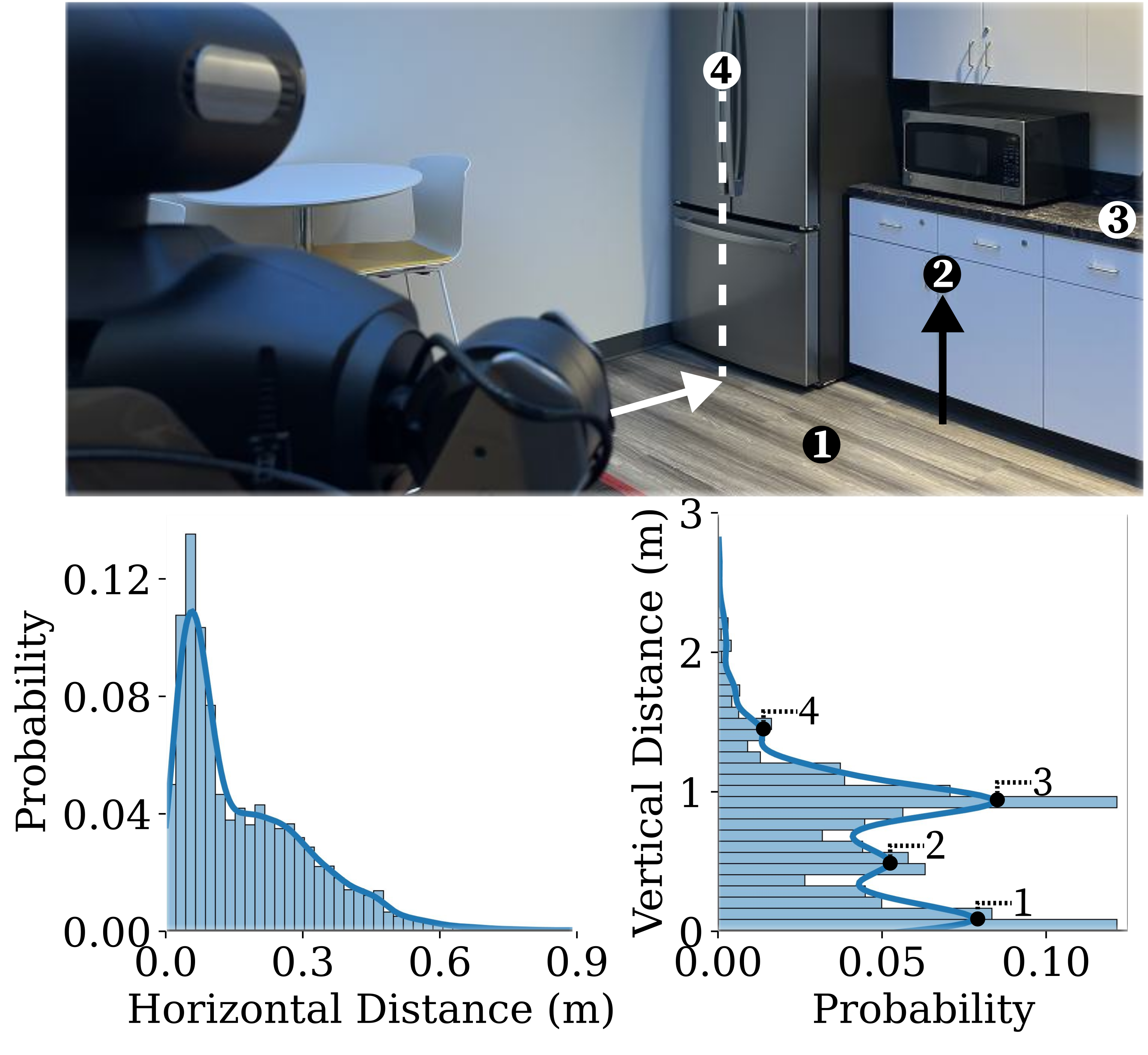
The BEHAVIOR-1K benchmark [8] motivates three requirements: using both arms together, navigating precisely while manipulating, and reaching objects from floor to overhead heights. Figure 2 shows multiple modes in object height, rather than one tabletop workspace. Hardware that expands these capabilities also enlarges the action space and complicates demonstration collection. BRS addresses both with JoyLo and a hierarchical action model. Table 1 retains the authors’ comparison with other systems; its capability entries refer to demonstrated learned policies, and its dollar symbols describe interface cost, not the full robot.
| BRS (Ours) | Mobile ALOHA [13] | TidyBot++ [14] | ACE [15] | BiDex [16] | HomeRobot [10] | TTT [17] | TeleMoMa [18] | RoboCopilot [19] | Open-TeleVision [20] | TRILL [21] | GR00T N1 [22] | ALOHA [23] | GELLO [24] | HATO [25] | FACTR [26] | ||
| Mobile manipulation | Humanoid manipulation | Stationary manipulation | |||||||||||||||
|
Simultaneous control of arms, torso, and mobile base |
✓ | ✗ | ✗ | ✗ | ✗ | ✗ | ✗ | ✓ | ✓ | ✗ | ✗ | ✗ | ✗ | ✗ | ✗ | ✗ | |
| Interface | Bimanual control | ✓ | ✓ | ✗ | ✓ | ✓ | ✗ | ✗ | ✓ | ✓ | ✓ | ✓ | ✓ | ✓ | ✓ | ✓ | ✓ |
| Torso control | ✓ | ✗ | ✗ | ✗ | ✗ | ✗ | ✗ | ✓ | ✓ | ✗ | ✗ | ✗ | ✗ | ✗ | ✗ | ✗ | |
| Single-operator mobile base control | ✓ | ✓ | ✓ | ✓ | ✗ | ✗ | ✗ | ✓ | ✓ | ✗ | ✓ | ✗ | ✗ | ✗ | ✗ | ✗ | |
| Untethered mobile base control | ✓ | ✗ | ✓ | ✓ | ✓ | ✗ | ✗ | ✓ | ✓ | ✗ | ✓ | ✗ | ✗ | ✗ | ✗ | ✗ | |
| Haptic feedback | ✓ | ✗ | ✗ | ✗ | ✗ | ✗ | ✗ | ✗ | ✓ | ✗ | ✗ | ✗ | ✗ | ✗ | ✗ | ✓ | |
| Cost(a) | $ | $ $ $ | $ $ | $ $ | $ | N.A. | N.A. | $ | $ $ $ | $ $ $ | $ | $ $ $ | $ $ $ | $ | $ | $ $ | |
| Capabilities(b) | Omnidirectional navigation | ✓ | ✗ | ✓ | ✗ | ✓ | ✗ | ✓ | ✓ | ✓ | ✗ | ✗ | ✗ | ✗ | ✗ | ✗ | ✗ |
| Bimanual coordination | ✓ | ✓ | ✗ | ✓ | ✓ | ✗ | ✓ | ✓ | ✓ | ✓ | ✓ | ✓ | ✓ | ✗ | ✓ | ✓ | |
| Ground-level reach | ✓ | ✗ | ✓ | ✓ | ✗ | ✗ | ✓ | ✓ | ✓ | ✗ | ✗ | ✗ | ✗ | ✗ | ✗ | ✗ | |
| Comfortable overhead reach(c) | ✓ | ✓ | ✗ | ✗ | ✗ | ✗ | ✓ | ✗ | ✗ | ✗ | ✗ | ✗ | ✗ | ✗ | ✗ | ✗ | |
| Operation in confined spaces | ✓ | ✗ | ✓ | ✗ | ✗ | ✗ | ✗ | ✗ | ✗ | ✗ | ✗ | ✗ | ✗ | ✗ | ✗ | ✗ | |
|
Coordinated whole-body manipulation involving hip, waist, and mobile base |
✓ | ✗ | ✗ | ✗ | ✗ | ✗ | ✗ | ✗ | ✗ | ✗ | ✗ | ✗ | ✗ | ✗ | ✗ | ✗ | |
| Learning-based method | ✓ | ✓ | ✓ | ✓ | ✓ | ✓ | ✗ | ✓ | ✓ | ✓ | ✓ | ✓ | ✓ | N.A. | ✓ | ✓ | |
| Algorithm | Novel algorithm | ✓ | ✗ | ✗ | ✗ | ✗ | ✗ | ✗ | ✗ | ✗ | ✗ | ✗ | ✓ | ✓ | N.A. | ✗ | ✓ |
|
Autoregressive whole- body action prediction |
✓ | ✗ | ✗ | ✗ | ✗ | ✗ | ✗ | ✗ | ✗ | ✗ | ✗ | ✗ | ✗ | N.A. | ✗ | ✗ | |
| Sensory observation modality |
Colored point cloud |
RGB | RGB | RGB | RGB |
Depth + semantic seg. |
RGB-D | RGB-D | RGB | RGB | RGB | RGB | RGB | N.A. |
RGB-D + tactile |
RGB | |
| Policy model backbone(d) | XF | XF | UNet | UNet | XF | RNN | N.A. | MLP/RNN | UNet | XF | RNN | XF | XF | N.A. | UNet | XF | |
| Open-source everything(e) | ✓ | ✓ | ✓ |
Hardware + teleop. |
Teleop. | ✓ | ✗ | Teleop. | ✗ | ✓ | ✓ |
Weights + finetuning |
✓ | ✓ | ✓ | ✓ | |
- (a)
Interface hardware cost. $: $0–$500; $$: $500–$1000; $$$: $1000+.
- (b)
We consider robot capabilities that are demonstrated by learned autonomous policies.
- (c)
Following Panero and Zelnik [27], we use () as the maximum height for comfortable overhead reach.
- (d)
Neural network architecture of the policy backbone. “XF” stands for Transformer.
- (e)
Everything includes the interface hardware, teleoperation code, algorithm code, and documentation.
2 JoyLo: Joy-Con on Low-Cost Kinematic-Twin Arms
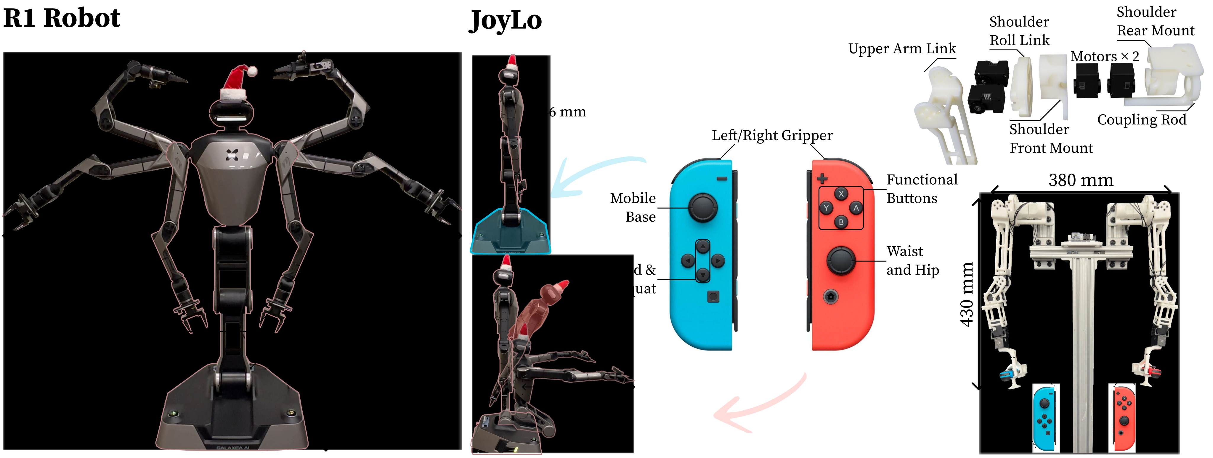
JoyLo pairs two kinematic leader arms with Nintendo Joy-Con controls for the torso, grippers, and mobile base. Its concrete implementation targets the R1 robot; adaptation to another embodiment is a design possibility rather than an evaluated transfer result.
Efficient Whole-Body Control
The operator physically moves miniature arms to command the corresponding robot joints. The left thumbstick controls base velocity, the right controls waist and hip, arrow keys adjust height, and triggers operate the grippers. This permits one operator to coordinate the entire body. Kinematic matching constrains arm commands to the robot’s joint structure, but does not by itself guarantee collision avoidance or safe interaction with the environment.
Rich User Feedback
Bilateral feedback regularizes leader-arm motion using robot joint positions and velocities, providing resistance when motion lags or contact occurs without additional force sensors. The source gives . Its final K term is described as damping but is not expanded into a complete velocity-dependent implementation law. This feedback mechanism should be distinguished from a calibrated measurement of environmental contact force.
Low Cost and Easy Accessibility
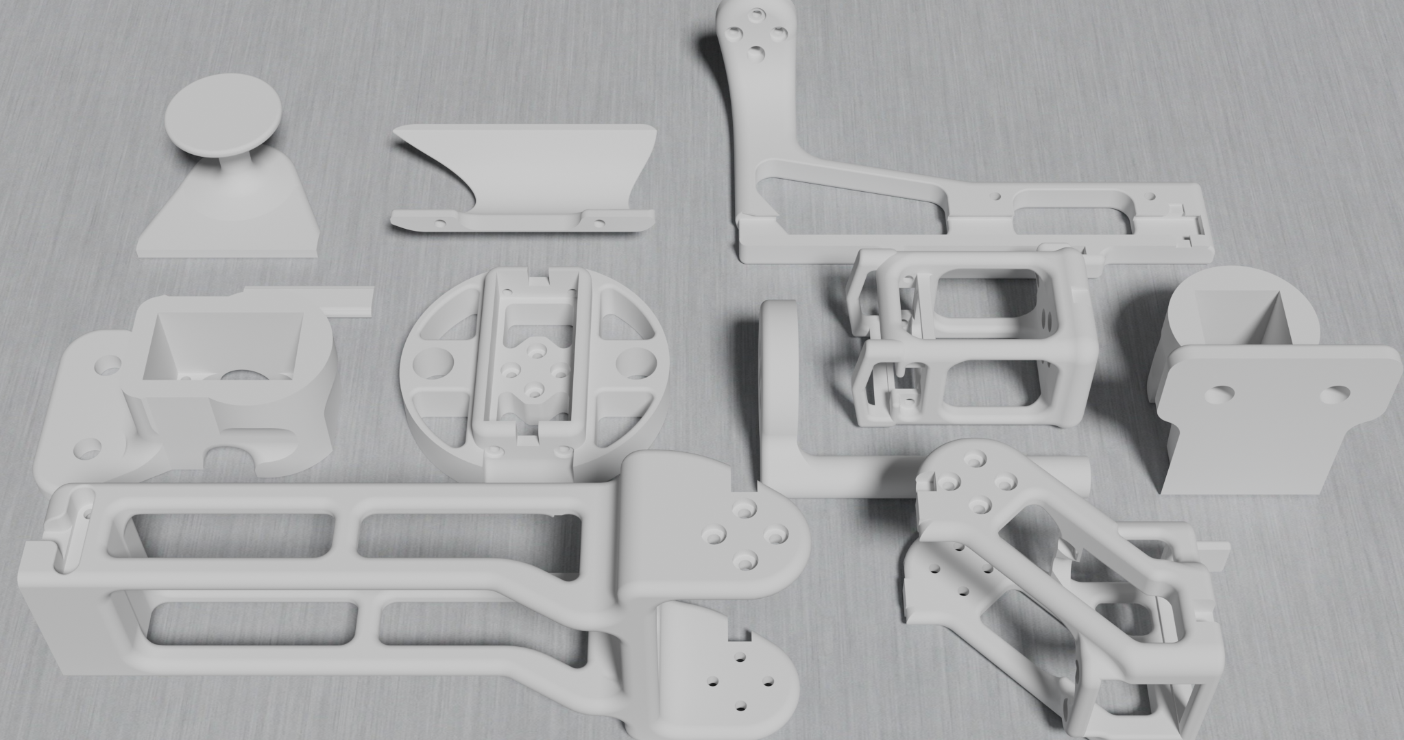
The interface uses printed links, low-cost Dynamixel motors, and Joy-Cons. Its bill of materials totals approximately $499.50 at the reported prices. That estimate excludes the R1 robot, cameras, workstation, printer, and assembly labor. Replaceable components and a Python controller support practical maintenance and data collection.
3 WB-VIMA: Whole-Body VIsuoMotor Attention Policy
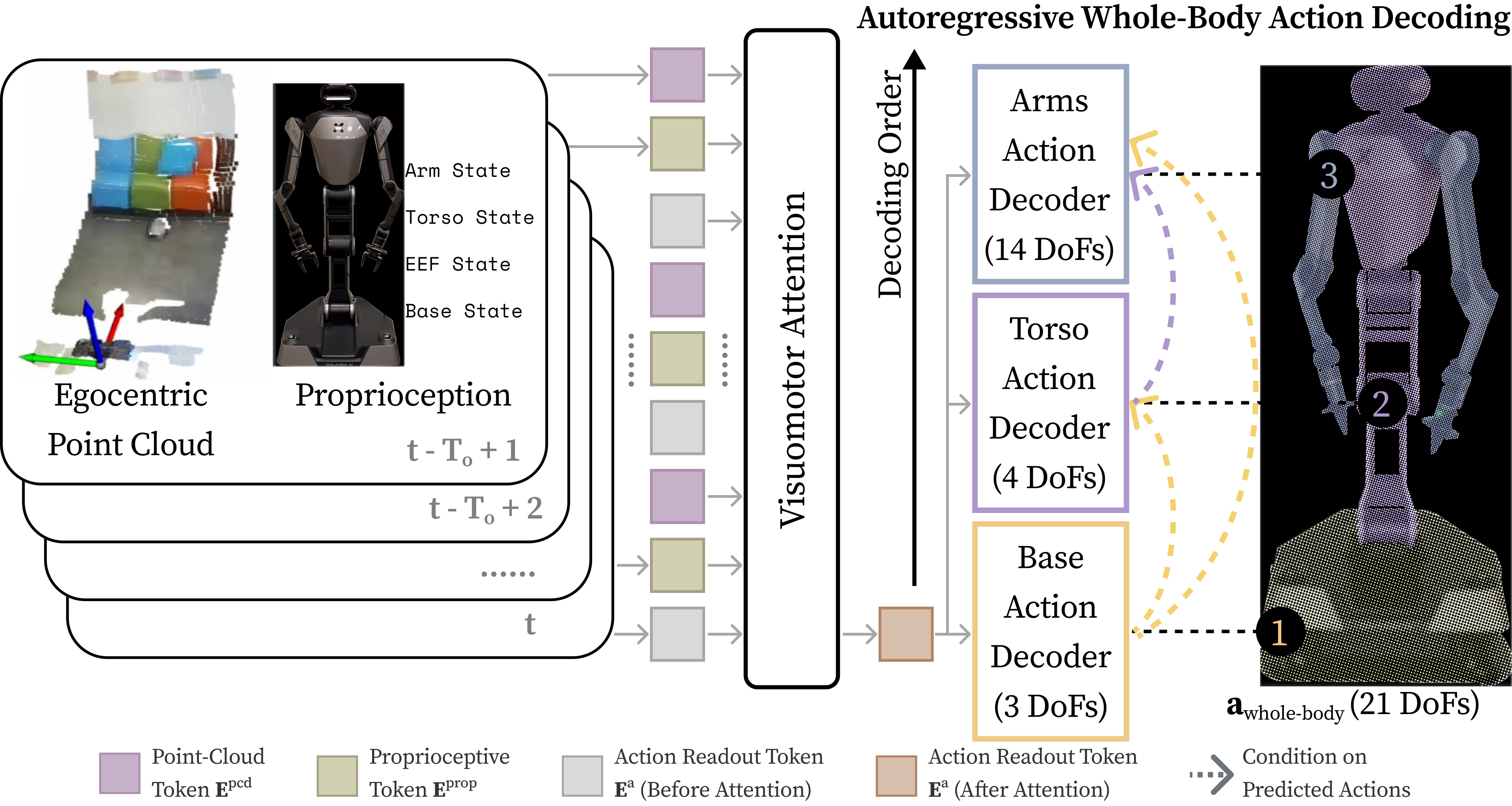
WB-VIMA separates observation encoding from action generation. A transformer combines recent visual and proprioceptive observations; three diffusion heads then decode body components in kinematic order.
Autoregressive Whole-Body Action Decoding
Small base or torso errors can displace the hands substantially; the paper illustrates that a 0.17 rad knee motion can shift an end-effector by about 0.14 m. WB-VIMA first predicts three base-velocity channels, conditions four torso-joint channels on that prediction, then conditions twelve arm joints and two gripper channels on both. Equation 1 preserves the three denoising updates for a 21-channel action trajectory. Autoregression is across body components, with trajectory chunks predicted by each diffusion head. It supplies learned coordination, not an analytic guarantee that downstream joints cancel every upstream error.
Equation 1
| (1) |
Multi-Modal Observation Attention
A PointNet [68] encodes colored point clouds and an MLP encodes joint/base state. For each observed time step, visual, proprioceptive, and action-readout tokens enter a causal attention sequence: the sequence S of point-cloud, proprioceptive, and action tokens over the observation window (displayed below). The last readout token conditions the action heads. The intended benefit is to use scene evidence alongside robot state rather than reproduce a sequence based mostly on proprioception.
Equation
Training and Deployment
Training minimizes the noise-prediction loss for each diffusion head and sums the three losses, following diffusion-policy methods [65]. The observation backbone runs once per inference call. Deployment reports 0.02 s effective latency on RTX 4090 hardware; recorded demonstrations and new policy actions run at 10 Hz, while the low-level controller repeats commands at 100 Hz. Asynchronous execution and discarded stale chunk actions help achieve that effective latency.
4 Experiments
Experiments evaluate task success, component ablations, teleoperation usability/data quality, and the contribution of base/torso motion. The physical task study and the simulator user study are separate evaluations.
Experiment Settings
There are 100 shelf, 103 toilet, 98 clothing, 138 post-party, and 122 trash demonstrations, totaling 561. Tasks randomize at least two factors among starting pose, object placement, instances, and distractors. Policies generally receive 15 runs per task. Sub-task evaluation resets after failures before continuing, whereas entire-task success requires completing the full sequence. Appendix Table A.XIII reports only eight RGB-DP clothing trials, an exception to the general fifteen-run description.
DP3, RGB diffusion policy, and ACT [23] are compared with WB-VIMA and human teleoperation. Recorded safety violations mean collisions or motor power loss under excessive force. Human rows have different trial counts from policies, so isolated human-versus-policy percentages are not matched-sample evidence of general superiority.
BRS enables various household activities, on which WB-VIMA consistently outperforms baseline methods ( 𝒬 𝟏 ).
The appendix gives full-task successes of 6/15 for post-party cleanup, 8/15 for toilet cleaning, 8/15 for trash, 14/15 for shelves, and 8/15 for clothing: 44/75 overall, or 58.7%. DP3 completes three shelf trials and no other full tasks; RGB-DP completes two shelf trials, and ACT none. WB-VIMA’s stronger sub-task results do not eliminate compounding failures. Its 93% peak belongs to the two-stage shelf task, not every household activity.
WB-VIMA records one safety violation in trash disposal and zero in the other four tasks. This is an empirical count over limited trials, not proof that point-cloud features inherently enforce safety. Baselines differ in color input, observation fusion, and action structure, so their overall gap cannot isolate one architectural choice. The paper’s headline 13×/21× full-task multipliers are not reproduced directly by the appendix’s reported macro-averages; the explicit task counts are retained rather than treating those multipliers as exact.
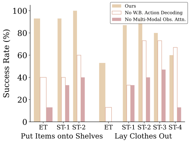
Synergistic whole-body action prediction and multi-modal feature extraction are key to WB-VIMA’s strong performance ( 𝒬 𝟐 ).
Removing hierarchical action decoding reduces shelf full-task success from 14/15 to 6/15 and clothing from 8/15 to 2/15. Removing multimodal attention reduces them to 2/15 and 0/15, with four clothing collisions. The shelf difference from 93% to 40% is about 53 percentage points. Figure 6 and the appendix retain all sub-task values and failure counts.
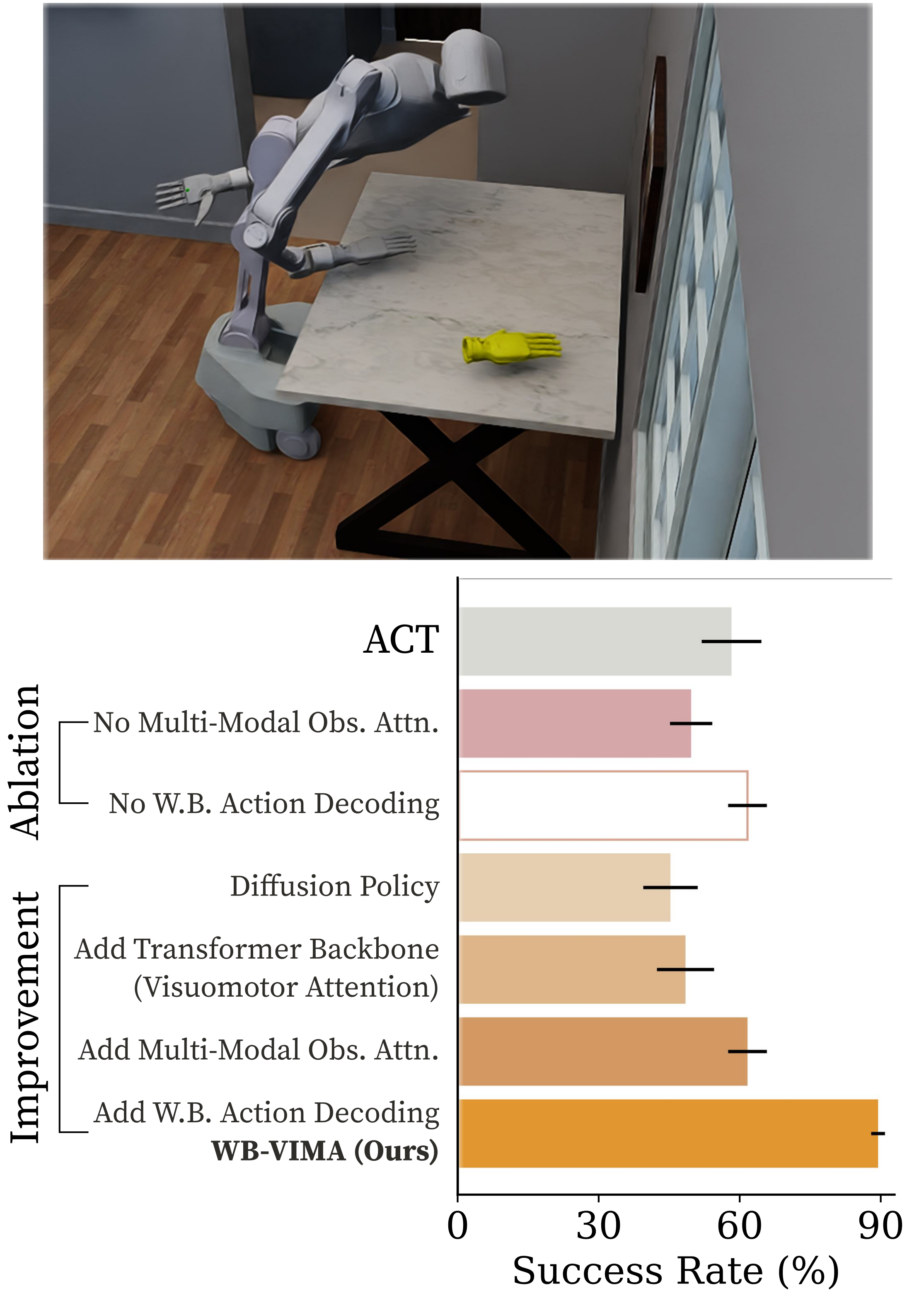
The simulated wiping study averages five runs of 100 rollouts and reports standard-deviation bars. Adding attention and hierarchical decoding progressively improves success. Its inputs and motion constraints differ from physical deployment: it uses a target position instead of camera observations and locks the base and two torso joints. This is a controlled coordination ablation, not another full visual mobile-manipulation benchmark.
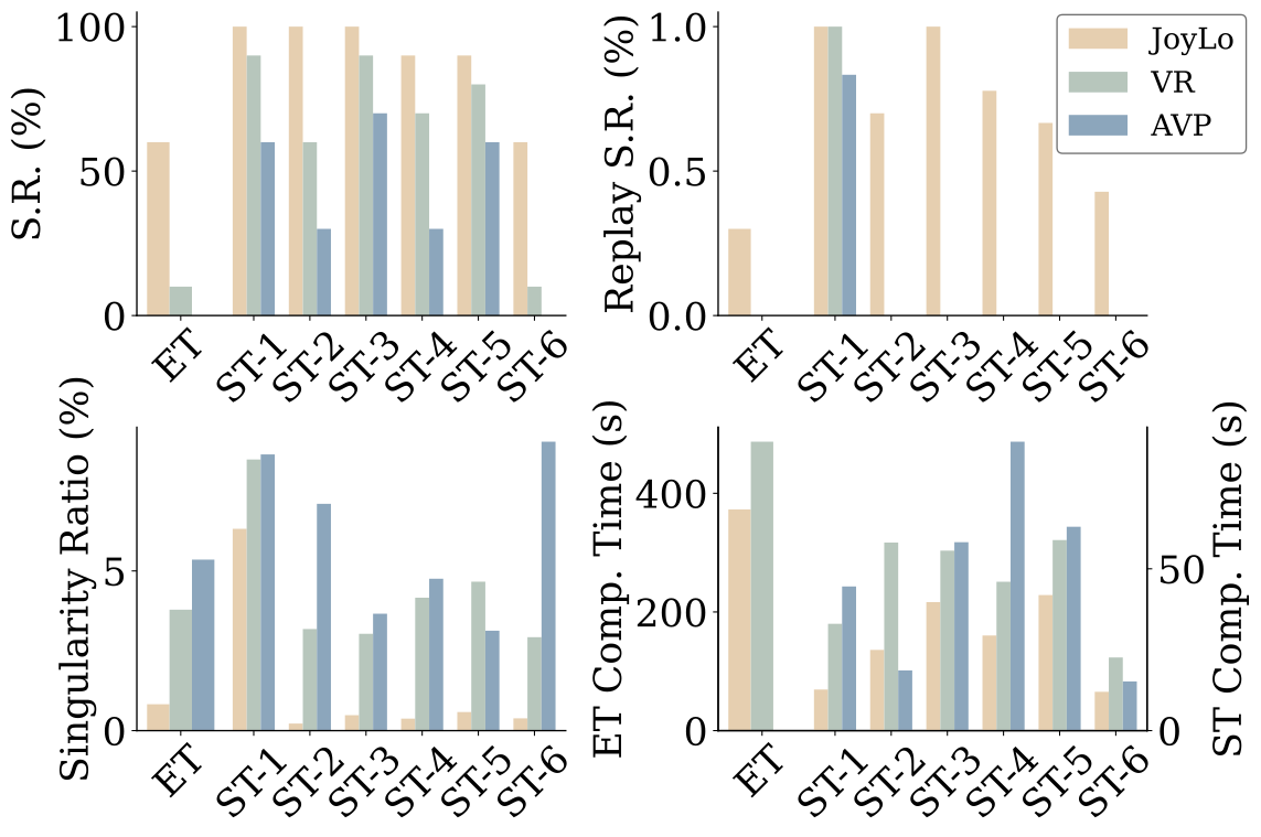
JoyLo is an efficient, user-friendly interface that provides high-quality data for policy learning ( 𝒬 𝟑 ).
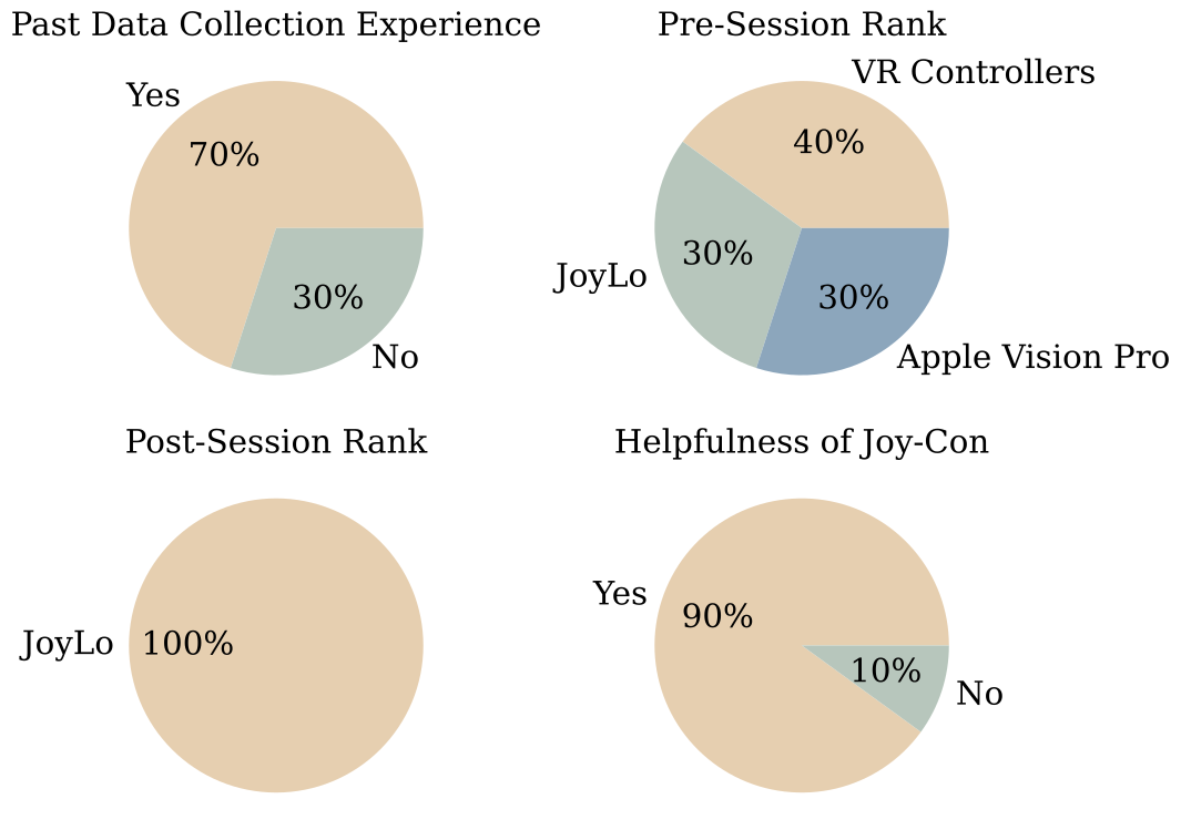
Ten participants compare JoyLo, VR controllers, and Apple Vision Pro in an OmniGibson post-party task. Interface order is randomized and each receives ten minutes of practice. JoyLo yields the highest task success, shortest reported times, and strongest open-loop replay results; the paper reports five times VR’s task success and 23% shorter median completion time. None finishes the entire task with Apple Vision Pro. All participants prefer JoyLo afterward, despite 70% initially favoring an IK-based option.
These results concern the implemented control mappings and a small simulator study. Replay success measures execution of recorded trajectories, not independently measured policy-learning gains. “Singularity” is measured using Jacobian conditioning for IK interfaces but excessive joint velocity for JoyLo, so the compared ratios use different operational definitions. Meta Quest 3 provides depth perception for both JoyLo and VR conditions.
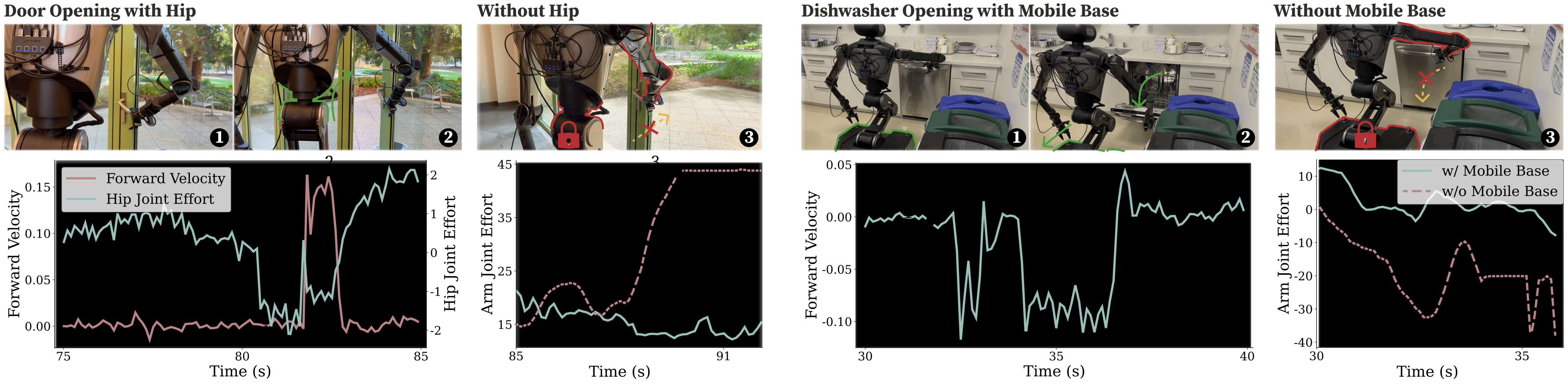
Coordinated torso and mobile base movements enhance maneuverability beyond stationary arms ( 𝒬 𝟒 ).
Figure 9 shows the robot moving its hip/base to open a door and backing its base to pull a dishwasher. Locking those components prevents opening and increases arm effort. These examples support the utility of whole-body motion for articulated objects. Additional recovery videos are qualitative examples rather than a quantified disturbance-robustness study.
5 Related Work
Related work covers household benchmarks and robotic systems, inexpensive robots and teleoperation devices, and planning/learning for whole-body manipulation. BRS combines leader-arm control, independent torso/base input, bilateral feedback, and a learned action hierarchy. Its comparison with Mobile ALOHA [13], DP3 [70], and earlier multimodal policies motivates those choices. The contribution is an integrated implementation and evaluated policy design, not a claim that prior systems lack all whole-body coordination.
6 Conclusion
The combination of suitable hardware, coordinated demonstrations, visual/state attention, and structured action generation improves the tested household tasks. The full-task success rate and limitations remain central to judging readiness: successful sub-tasks and individual demonstrations do not establish reliable general home assistance.
7 Limitations
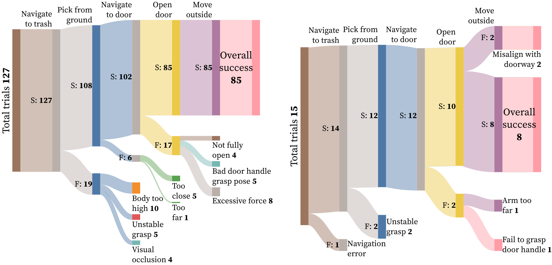
The four limitations below concern partial observability, compounding errors, perception quality, and the scope of the training distribution. Figure 10 preserves the detailed trash-task failure flows.
Mismatched camera field of view between robot and operator.
Operators view the robot from outside while policies receive onboard cameras. The operator must keep targets visible to those cameras and avoid appearing in their view; otherwise demonstrations may rely on information unavailable to the policy. Active perception or a shared robot-view interface is proposed as future work.
Compounding errors in long-horizon, multi-stage tasks.
Errors accumulate across long sequences even when individual sub-task success is high. Human correction data or model-based task planning may help, but are not evaluated remedies here. Figure 10’s human trash flow reports 85 successes out of 127, whereas Table A.XI reports 96/127; these source results disagree and should not be merged into a single resolved success estimate. The policy flow’s eight successes out of fifteen agrees with the table.
Imperfect point cloud observations.
Stereo point clouds degrade with lighting changes and reflective surfaces. Daytime training need not generalize to night. Improving stereo with FoundationStereo [154] is suggested, not tested in the reported system.
Robot-specific training data.
Training data comes only from the R1 embodiment and the available task scenes. Cross-robot transfer, broad scene-level generalization, pretrained vision-language-action models, and synthetic/human data are future directions. The paper does not establish zero-shot transfer to unfamiliar homes or embodiments.
Acknowledgments
The authors acknowledge technical collaborators, Galaxea hardware support, study participants, and Stanford facilities, with support from Stanford HAI, Schmidt Futures, NSF, and ONR programs.
Appendix A Robot Hardware Details
The hardware appendix records the concrete platform, measured capabilities, sensor setup, and workstation communication required to reproduce this implementation.
A.1 Robot Platform
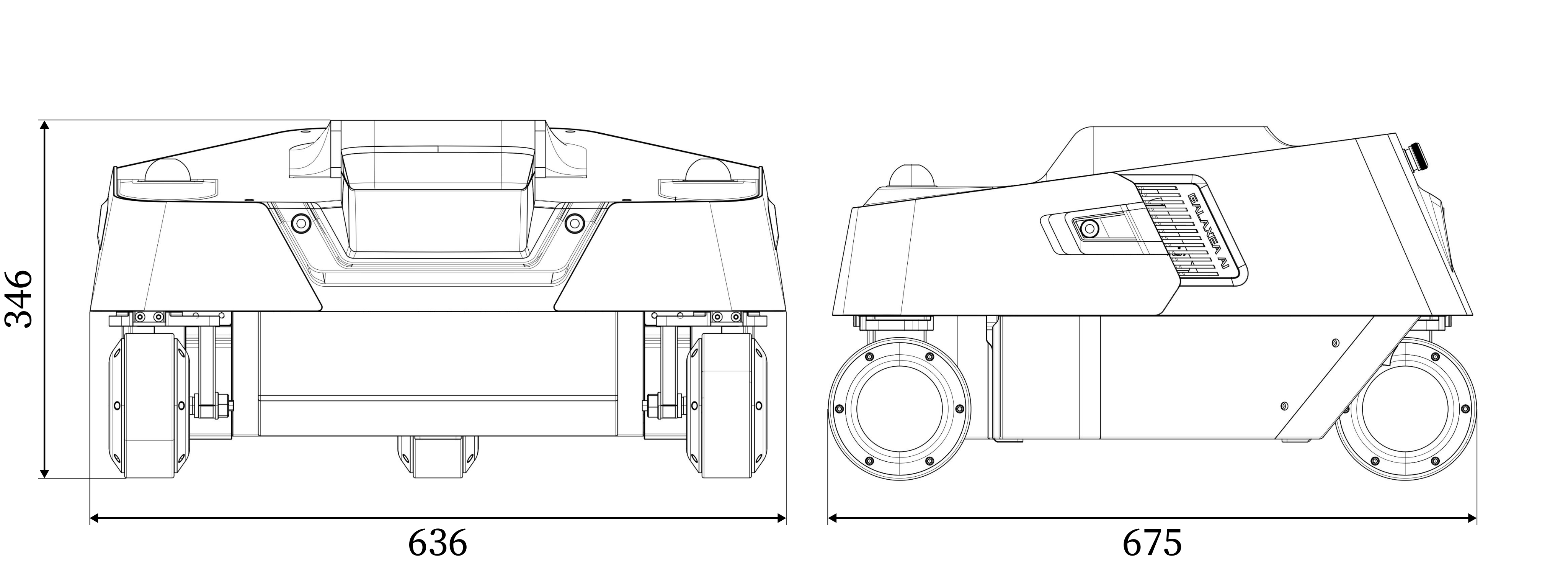
R1 has two six-joint arms with parallel grippers, a four-joint torso, and an omnidirectional wheeled base. The authors’ tests report 5 kg payload per arm, ground-to-2 m vertical reach, and up to 2.06 m horizontal reach with the torso. Base limits include 1.5 m/s translation, 3 rad/s yaw, and 30 mm ground clearance. These are reported platform capabilities, not the velocities or loads used in every demonstration.
A.2 Hardware Specifications
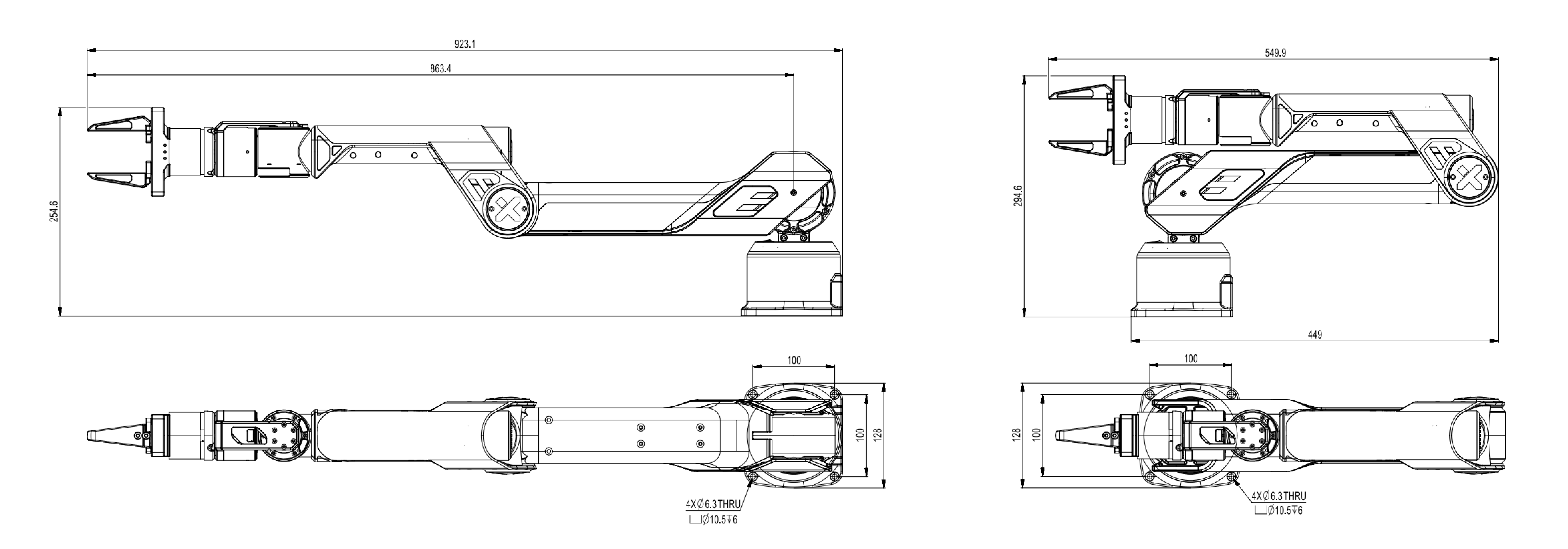
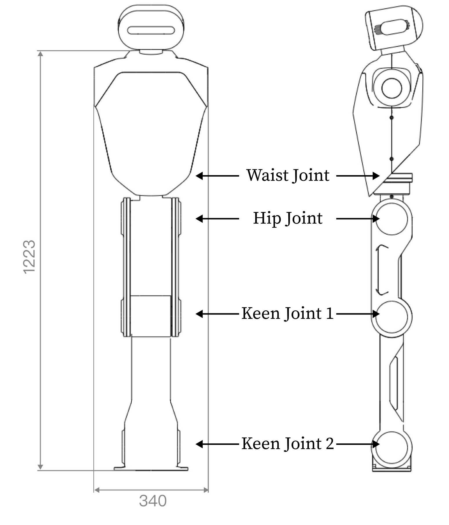
Figure A.1 retains all arm, torso, and base dimension drawings and labels. Tables A.I–A.III retain joint, mobility, and camera specifications.
A.2.1 Arms
Each arm has 923 mm full reach and 128 mm width. Joint impedance gains are Kp = [140, 200, 120, 20, 20, 20] and Kd = [10, 50, 5, 1, 1, 0.4]. Grippers span 0–100 mm with a reported 100 N rated force; target width is converted into motor current.
A.2.2 Torso
The torso combines waist yaw, hip pitch, and two knee-like joints. Fully extended dimensions are 340 mm wide and 1,223 mm high excluding the head. Table A.I retains each angular range and the 108 N·m rated/304 N·m maximum motor torque specifications.
| Parameter | Value |
|---|---|
| Waist Joint Range (Yaw) | () |
| Hip Joint Range (Pitch) | () () |
| Knee Joint 1 Range | () () |
| Knee Joint 2 Range | () () |
| Rated Motor Torque | |
| Maximum Motor Torque |
A.2.3 Mobile Base
Three wheel motors and three steering motors provide planar x/y velocity and yaw control. Table A.II retains distinct acceleration limits: 2.5 m/s² forward, 1.0 m/s² lateral, and 1.0 rad/s² yaw. The broad prose claim of 2.5 m/s² horizontal acceleration should not be applied to every direction.
| Parameter | Value |
|---|---|
| Forward Velocity Limit | |
| Lateral Velocity Limit | |
| Yaw Rotation Velocity Limit | |
| Forward Acceleration Limit | |
| Lateral Acceleration Limit | |
| Yaw Rotation Acceleration Limit |
A.3 Onboard Sensors and Computing
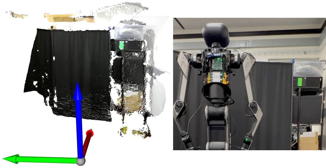
A head ZED 2 and two wrist ZED-Mini cameras stream RGB-D data at 60 Hz; a rear RealSense T265 supplies odometry at 200 Hz. Forward kinematics updates camera poses at 500 Hz. The source fuses camera point clouds as , then crops spatially and uses farthest-point sampling. Although the prose names a base-to-camera transform, the displayed row-vector operation must be implemented with the appropriate camera-to-base convention. A Jetson Orin handles onboard sensing and processing.
| Parameter | Value |
|---|---|
| RGB-D Cameras | |
| Frequency | |
| Image Resolution | 1344376 |
| ZED Depth Mode | PERFORMANCE |
| Head Camera Min Depth | 0.2 |
| Head Camera Max Depth | 3 |
| Wrist Camera Min Depth | 0.1 |
| Wrist Camera Max Depth | 1 |
| Tracking Camera | |
| Odometry Frequency | |
A.4 Communication Scheme
ROS camera/state nodes communicate with a workstation master over a local network. The workstation subscribes to observations, runs policy/control logic, and sends commands through ROS topics; onboard sensing does not imply onboard policy inference.
Appendix B JoyLo Details
JoyLo’s implementation details include printable hardware, communication rates, impedance control, and recorded data fields.
B.1 Hardware Components
Two arms take a reported thirteen printer-hours and 317 g of PLA. Table A.IV retains every component, quantity, supplier, and price. Sixteen Dynamixel motors account for $382.40, Joy-Cons $70, and the USB converter $32.10. Motor states are read at roughly 400–500 Hz and Joy-Cons communicate over Bluetooth at 66 Hz.
| Item No. | Part Name | Description | Quantity | Unit Price ($) | Total Price ($) | Supplier |
| 1 | Dynamixel XL330-M288-T | JoyLo arm joint motors | 16 | 23.90 | 382.40 | Dynamixel |
| 2 | Nintendo Joy-Con | JoyLo hand-held controllers | 1 | 70 | 70 | Nintendo |
| 3 | Dynamixel U2D2 | USB communication converter for controlling Dynamixel motors | 1 | 32.10 | 32.10 | Dynamixel |
| 4 | 5V DC Power Supply | Power supply for Dynamixel motors | 1 | <10 | <10 | Various |
| 5 | 3D Printer PLA Filament | PLA filament for 3D printing JoyLo arm links | 1 | 5 | 5 | Various |
| Total Cost: $499.5 | ||||||
B.2 Controller Implementation
The Python interface sends torso/arm joint targets, gripper widths, and base velocities at 100 Hz. Bilateral leader-arm control uses current-based impedance with proportional gains 0.5 and derivative gains 0.01 for each of six joints. Coupled motors increase torque at load-bearing leader-arm joints. Pseudocode 1 is preserved exactly; its right-gripper command repeats the left-gripper target variable, which should be checked before reuse rather than silently treated as a correct independent command.
B.3 Data Collection
Data is recorded at 10 Hz while control runs at 100 Hz. Joy-Con buttons start, pause, save, or discard a recording. Saved observations include color, depth, point clouds, joints, odometry, and commands. The full controller listing below retains original indentation and all source text.
from brs_ctrl.robot_interface import R1Interface

# instantiate the controller
robot = R1Interface(...)
# send a control command
robot.control(
    # the torso and arms commands are target joint positions
    arm_cmd={
        "left": left_arm_target_q,
        "right": right_arm_target_q,
    },
    gripper_cmd={
        "left": left_gripper_target_width,
        "right": left_gripper_target_width,
    },
    torso_cmd=torso_target_q,
    # the mobile base commands are target velocities
    base_cmd=mobile_base_target_velocity,
)
Appendix C Model Architectures, Policy Training, and Deployment Details
This appendix supplies the observation/action architecture, baseline differences, optimizer schedules, and asynchronous deployment details.
C.1 Preliminaries
The formulation describes a state-to-action policy and trains it by imitation through diffusion noise prediction.
Problem Formulation
The paper introduces an MDP with states, actions, transition dynamics, initial-state distribution, and reward. The implemented policy training is behavior cloning of demonstrations; an MDP notation or reward symbol does not imply reinforcement-learning optimization in these experiments.
Denoising Diffusion for Policy Learning
A DDPM progressively corrupts data with Gaussian noise and learns a reverse process conditioned on observations. Equation A.1 preserves the reverse Gaussian update and scheduled variance. Each action head predicts the noise needed to denoise an action trajectory, following prior diffusion policies.
Equation A.1
| (A.1) |
C.2 WB-VIMA Architecture
WB-VIMA uses 256-dimensional observation features, a short causal observation history, and compact diffusion heads for eight future action steps.
C.2.1 Observation Encoder
Each of 4,096 points contains RGB plus XYZ. Colors are divided by 255, and coordinates by task-specific spatial limits. PointNet uses two hidden layers of width 256, GELU, and a 256-dimensional output. The proprioception MLP receives 21 values, uses three hidden layers of width 256 and ReLU, and emits 256 features. Table A.V retains the full configuration.
C.2.2 Multi-Modal Observation Attention
The transformer has width 256, two layers, eight heads, dropout 0.1, and GEGLU activation. Observation window To = 2 is shared across methods. Action-readout tokens attend to preceding observations; the last readout becomes the diffusion condition. Table A.VI preserves these settings.
C.2.3 Autoregressive Whole-Body Action Decoding
Three separate UNets predict base, torso, and arm/gripper chunks in that order, using action horizon Ta = 8. Higher-body heads receive completed lower-body predictions. The observation backbone runs once, while denoising iterates in the smaller heads. Table A.VII reports widths [64, 128], kernel size 2, five GroupNorm groups, and diffusion embedding size 8. Five groups do not evenly divide the listed widths, so the actual normalization implementation should be checked rather than assuming that table is a complete executable specification.
C.3 Baselines Architectures
DP3 shares the PointNet/proprioception encoders but omits RGB channels and fuses features with a two-layer 512-unit MLP before flat 21-channel diffusion. RGB-DP uses pretrained ResNet-18 visual features with a 512-dimensional output. ACT follows its recommended hyperparameters. Thus color, fusion architecture, and action factorization differ across baselines; the targeted ablations provide more direct evidence for individual WB-VIMA components.
C.4 Policy Training Details
Data splits are 90% training and 10% validation. Methods train for equal steps and use the final checkpoint. AdamW uses learning rate 7×10⁻⁴, weight decay 0.1, 1,000 warm-up steps, cosine decay over 300,000 steps, and minimum rate 5×10⁻⁶. Training uses 100 DDPM noise steps; inference uses 16 DDIM steps. Multi-GPU training employs RTX A5000, RTX 4090, and A40 devices. Table A.VIII retains all schedule values.
| Hyperparameter | Value |
|---|---|
| Learning Rate | |
| Weight Decay | 0.1 |
| Learning Rate Warm Up Steps | 1000 |
| Learning Rate Cosine Decay Steps | 300,000 |
| Minimal Learning Rate |
C.5 Policies Deployment Details
Policy inference runs continuously on a workstation while the controller executes an existing action chunk. When switching chunks, early actions that became stale during inference are discarded. This addresses effective execution delay; the reported 0.02 s figure should not be interpreted as a complete breakdown of all sensor/network/compute latency.
Appendix D Task Definition and Evaluation Details
The final appendix defines each task, its randomization and demonstrations, the numerical evaluations, the constrained simulation ablation, and the user-study protocol.
D.1 Task Definition
Post-party cleanup has six stages: navigate to dishwasher, open it, move to the table, collect bowls, return, and load/close; 138 demonstrations average 210 s. Toilet cleaning has six stages from sponge pickup and lid opening through wiping, closing, and flushing; 103 demonstrations average 120 s. Trash disposal has four stages from bag pickup through door opening and outside disposal; 122 demonstrations average 130 s.
Shelving has two stages, floor-box pickup and placement on an available shelf; 100 demonstrations average 60 s. Clothing has four stages, wardrobe opening, jacket retrieval, laying it on a sofa bed, and closing the wardrobe; 98 demonstrations average 120 s. All randomize initial position, with task-specific changes to objects, placements, free shelf space, contents, or distractors. These randomizations are narrower than entirely new household layouts.
D.2 Policy Evaluation Results
Tables A.IX–A.XIII retain every success percentage, numerator/denominator, baseline, ablation row, and safety count. Human denominators vary across stages, and RGB-DP clothing has eight trials. Sub-task resets mean those columns are not conditional survival probabilities whose product must reproduce entire-task success.
D.3 Simulation Ablation Details
The OmniGibson wiping ablation uses 100,000 cuRobo-generated trajectories. The base and first two torso joints are locked, and the target hand position replaces camera inputs while proprioception remains. The robot must reach the target while maintaining table contact. These simplifications isolate control/fusion choices but limit inference about visual navigation or unconstrained whole-body behavior.
D.4 User Study Details
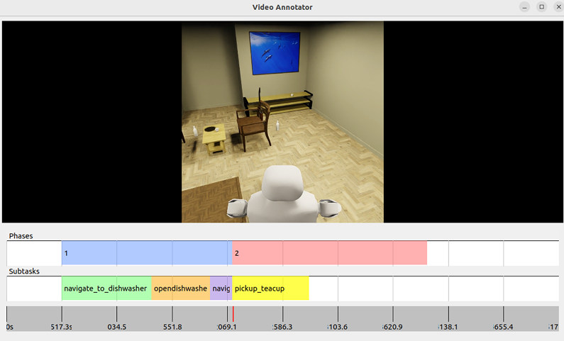
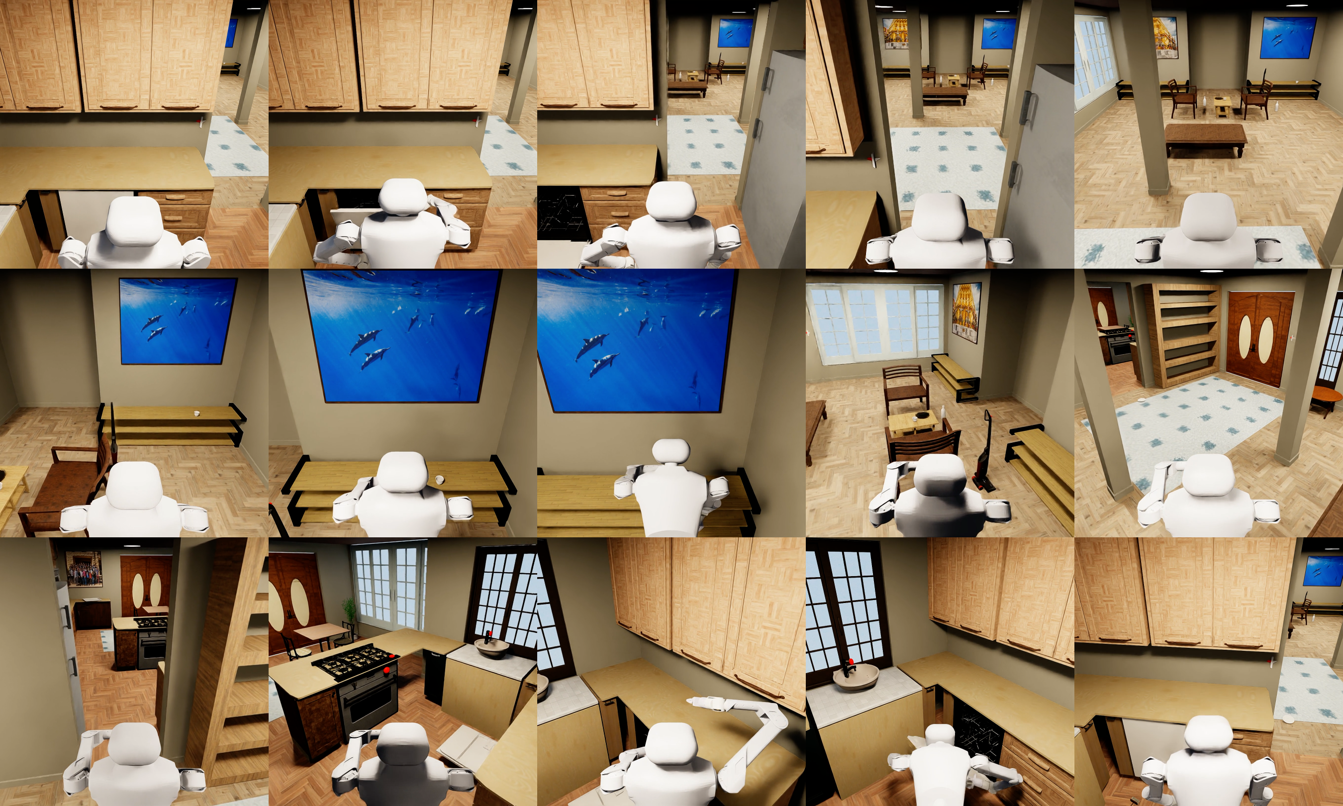
Ten participants test all three interfaces in randomized order with ten minutes of practice per interface. JoyLo and VR users wear a Meta Quest 3 for depth perception. Rollouts are manually segmented and labeled with the GUI in Figure A.5; Figure A.6 preserves the complete illustrated successful sequence. IK interfaces use a Jacobian-condition threshold to identify singularities, while JoyLo uses excessive joint speed, with threshold values not specified here.
The five survey questions ask about prior collection experience, expected and observed usability, whether physically holding the leader arms helped, and whether torso/base thumbsticks improved control. Figure A.4 retains the reported demographics and responses, including unanimous post-study preference for JoyLo and 90% reporting helpful Joy-Con control. Preferences and the simulator performance are evidence about this study population and mappings, not universal rankings of every teleoperation implementation.
| ET | ST-1 | ST-2 | ST-3 | ST-4 | ST-5 | ST-6 | Safety Violations | |
|---|---|---|---|---|---|---|---|---|
| Human Teleop. |
68% (50/73) |
100% (73/73) |
93% (69/74) |
100% (69/69) |
89% (64/72) |
94% (60/64) |
88% (53/60) |
N/A |
| Ours |
40% (6/15) |
100% (15/15) |
80% (12/15) |
80% (12/15) |
73% (11/15) |
93% (14/15) |
93% (14/15) |
0 |
| DP3 [70] |
0% (0/15) |
80% (12/15) |
7% (1/15) |
27% (4 / 15) |
7% (1/15) |
33% (5/15) |
40% (6/15) |
13 |
| RGB-DP [65] |
0% (0/15) |
93% (14/15) |
0% (0/15) |
0% (0/15) |
7% (1/15) |
7% (1/15) |
20% (3/15) |
2 |
| ACT [23] |
0% (0/15) |
80% (12/15) |
0% (0/15) |
0% (0/15) |
0% (0/15) |
0% (0/15) |
0% (0/15) |
2 |
| ET | ST-1 | ST-2 | ST-3 | ST-4 | ST-5 | ST-6 | Safety Violations | |
|---|---|---|---|---|---|---|---|---|
| Human Teleop. |
61% (100/164) |
91% (150/164) |
72% (106/148) |
99% (104/105) |
100% (103/103) |
98% (102/104) |
98% (100/102) |
N/A |
| Ours |
53% (8/15) |
100% (15/15) |
80% (12/15) |
100% (15/15) |
100% (15/15) |
100% (15/15) |
73% (11/15) |
0 |
| DP3 [70] |
0% (0/15) |
100% (15/15) |
47% (7/15) |
93% (14/15) |
0% (0/15) |
13% (2/15) |
0% (0/15) |
0 |
| RGB-DP [65] |
0% (0/15) |
93% (14/15) |
13% (2/15) |
7% (1/15) |
7% (1/15) |
0% (0/15) |
20% (3/15) |
2 |
| ACT [23] |
0% (0/15) |
20% (3/15) |
0% (0/15) |
0% (0/15) |
0% (0/15) |
0% (0/15) |
0% (0/15) |
0 |
| ET | ST-1 | ST-2 | ST-3 | ST-4 | Safety Violations | |
|---|---|---|---|---|---|---|
| Human Teleop. |
76% (96/127) |
91% (116/128) |
100% (124/124) |
85% (106/125) |
100% (115/115) |
N/A |
| Ours |
53% (8/15) |
80% (12/15) |
100% (15/15) |
87% (13/15) |
87% (13/15) |
1 |
| DP3 [70] |
0% (0/15) |
60% (9/15) |
53% (8/15) |
20% (3/15) |
7% (1/15) |
9 |
| RGB-DP [65] |
0% (0/15) |
20% (3/15) |
7% (1/15) |
7% (1/15) |
7% (1/15) |
3 |
| ACT [23] |
0% (0/15) |
0% (0/15) |
0% (0/15) |
0% (0/15) |
0% (0/15) |
5 |
| ET | ST-1 | ST-2 | Safety Violations | |
|---|---|---|---|---|
| Human Teleop. |
89% (93/104) |
90% (94/104) |
100% (93/93) |
N/A |
| Ours |
93% (14/15) |
93% (14/15) |
100% (15/15) |
0 |
| DP3 [70] |
20% (3/15) |
27% (4/15) |
47% (7/15) |
0 |
| RGB-DP [65] |
13% (2/15) |
20% (3/15) |
40% (6/15) |
0 |
| ACT [23] |
0% (0/15) |
0% (0/15) |
33% (5/15) |
1 |
| Ours w/o W.B. Action Denoising |
40% (6/15) |
40% (6/15) |
60% (9/15) |
0 |
| Ours w/o Multi-Modal Obs. Attn. |
13% (2/15) |
33% (5/15) |
40% (6/15) |
0 |
| ET | ST-1 | ST-2 | ST-3 | ST-4 | Safety Violations | |
|---|---|---|---|---|---|---|
| Human Teleop. |
50% (54/108) |
56% (60/108) |
93% (56/60) |
96% (54/56) |
100% (54/54) |
N/A |
| Ours |
53% (8/15) |
87% (13/15) |
93% (14/15) |
80% (12/15) |
60% (9/15) |
0 |
| DP3 [70] |
0% (0/15) |
13% (2/15) |
13% (2/15) |
27% (4/15) |
27% (4/15) |
7 |
| RGB-DP [65] |
0% (0/8) |
13% (1/8) |
25% (2/8) |
13% (1/8) |
13% (1/8) |
3 |
| ACT [23] |
0% (0/15) |
0% (0/15) |
0% (0/15) |
0% (0/15) |
0% (0/15) |
1 |
| Ours w/o W.B. Action Denoising |
13% (2/15) |
33% (5/15) |
73% (11/15) |
73% (11/15) |
67% (10/15) |
0 |
| Ours w/o Multi-Modal Obs. Attn. |
0% (0/15) |
33% (5/15) |
40% (6/15) |
47% (7/15) |
13% (2/15) |
4 |