At a glance
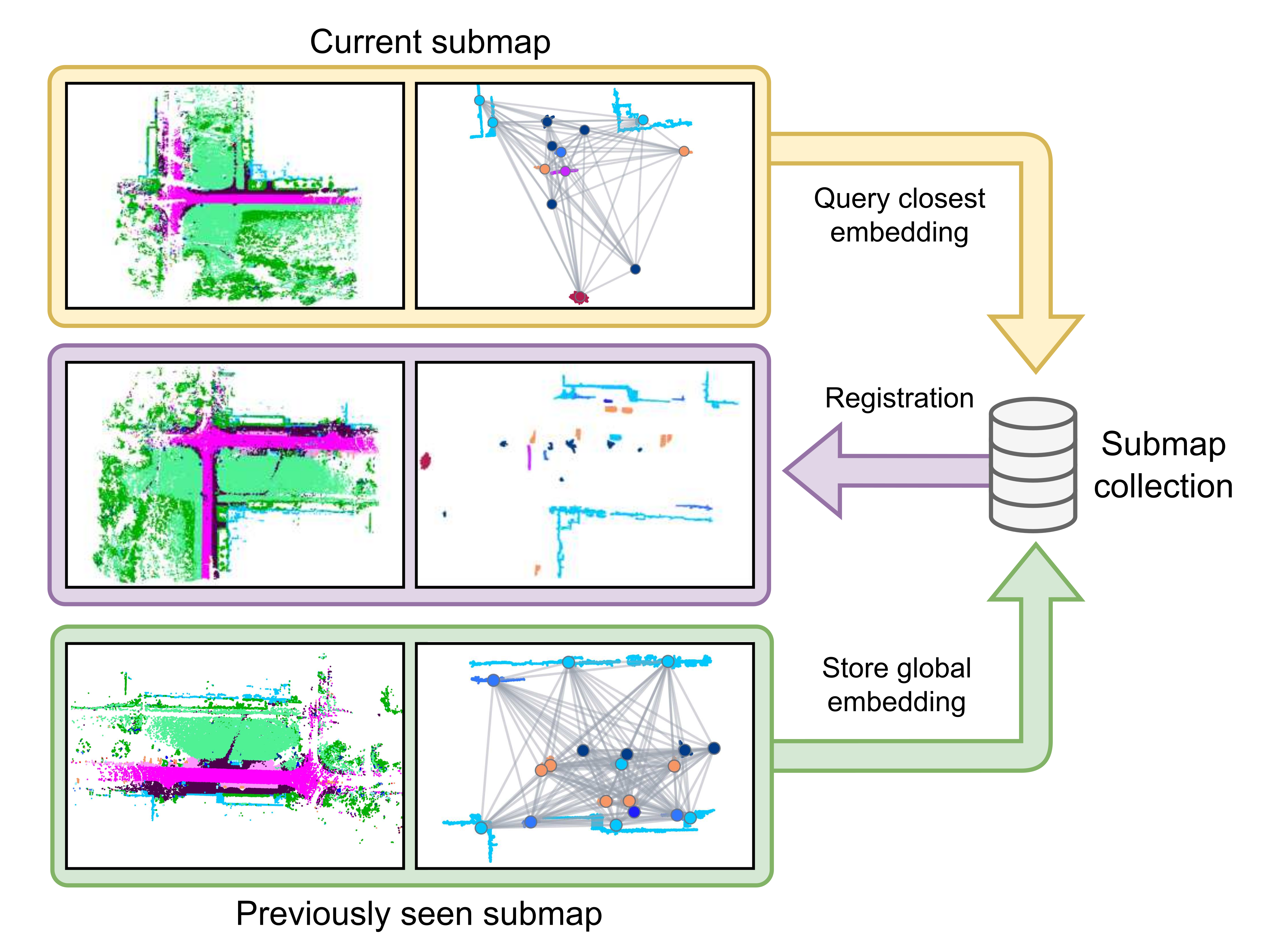
REGRACE aggregates LiDAR scans into semantic submaps, encodes object instances with rotation-invariant features, and adds spatial context through a graph network. One global descriptor retrieves candidate revisits; geometric consistency then selects and validates a candidate before object-based registration.
On KITTI, the method is competitive at short range and particularly strong for 20 m revisit thresholds. Its small set of object keypoints reduces measured registration and re-ranking time. Performance is not uniformly best: EgoNN remains stronger on several short-range metrics and has slightly higher registration success on sequence 08. The paper’s timing measures selected pipeline stages rather than a complete sensor-to-map latency budget.
I INTRODUCTION
Re-localization asks whether the robot has returned to a mapped region and, if so, estimates the rigid six-degree-of-freedom transform. Single-scan descriptors are sensitive to occlusion and viewpoint. Combining nearby scans exposes more of the same objects, while representing each object by one descriptor reduces the number of matching keypoints.
REGRACE couples compact global retrieval with explicit geometric verification. This addresses different questions: which stored submaps look promising, and whether their matched objects support a consistent alignment. The contribution is evaluated on automotive KITTI sequences; long-range refers to revisit separation within the tested 20 m setting, not arbitrary distant or cross-domain localization.
II RELATED WORK
The relevant literature covers point-cloud and object-based retrieval, geometric verification, and robust registration.
II-A Point cloud-based Place Recognition
Global descriptors support efficient database queries, while pairwise graph-similarity networks require more expensive comparisons. Dense point-cloud encoders preserve rich geometry but may produce many keypoints. REGRACE pools object descriptors into one queryable submap embedding, retaining local features for later matching.
Object-centric methods such as SemSegMap and graph-based methods such as SGPR motivate this representation. The added graph context distinguishes scenes containing similar object types in different spatial arrangements.
II-B Metric Evaluation
A descriptor-distance threshold need not correspond consistently to physical revisit distance. Re-ranking can change which candidate is first without making its embedding closer to the query. REGRACE therefore uses a geometric score both to choose among retrieved candidates and to classify a revisit. This criterion remains conditional on retrieving a suitable candidate and finding reliable correspondences.
II-C Registration
Robust registration typically first matches sparse descriptors, then estimates a transform despite outliers. RANSAC supplies a coarse alignment and ICP refines it. REGRACE reduces the coarse matching problem to object centers and later applies dense refinement only to selected inlier objects.
III METHODOLOGY
The pipeline builds semantic object graphs, learns local and global features, retrieves nearby embeddings, evaluates geometric consistency, and refines the selected transform.
III-A Problem Formulation
Each submap is a point cloud in its own frame with a pose in a common world frame. Given a new submap, the method searches previous submaps for the same physical region and estimates the rigid transform aligning a selected pair. Existing SLAM poses are used during submap construction.
III-B Overview
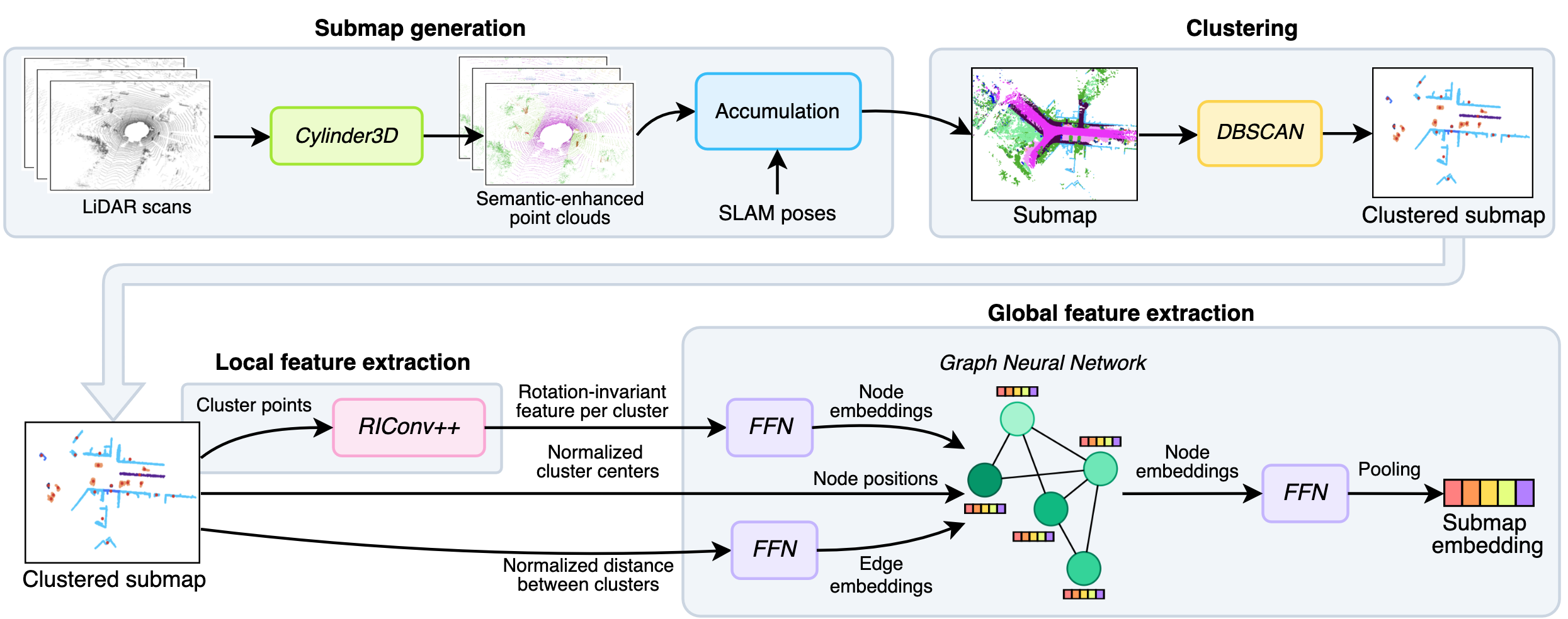
Cylinder3D labels scans; SLAM poses merge them into submaps; DBSCAN separates same-class points into instances. RIConv++ encodes each object, an equivariant graph network adds neighborhood context, and pooling produces a global descriptor.
At query time, retrieve the closest global descriptors, select the most geometrically consistent candidate, and register it using the local object features. The complete architecture diagram preserves the feed-forward connections between these stages.
III-C Submap Generation
Scans are accumulated until their displacement from the first scan reaches the 20 m submap limit. The middle scan defines the submap frame. Points are discretized into 10 cm voxels, and semantic probabilities are averaged within each voxel to reduce classification noise. This expands coverage but also inherits pose-estimation and semantic-label errors.
III-D Local Features
DBSCAN clusters same-label points into object instances. Road, sidewalk, ground, terrain, unlabeled, outlier, and other-object categories are excluded. Each object center becomes a keypoint, and RIConv++ maps its geometry to a 128-dimensional feature.
Each cluster supplies 1024 farthest-sampled points; smaller clusters are padded with additional sampled points from that cluster. Rotation-invariant object features reduce orientation sensitivity, but do not guarantee robustness to segmentation changes or partial observations. The reported clustering parameters are preserved in the implementation section.
III-E Global descriptor
Before pooling, object descriptors exchange information through a graph so the global descriptor reflects spatial arrangement as well as individual object appearance.
III-E 1 Graph Construction
Every object is connected to every other object. Edge features encode center-to-center distance normalized by a training-set 95th-percentile object-distance scale. Full connectivity allows large peripheral objects, such as buildings, to inform central nodes, such as cars and poles.
The compact node set makes this practical in the reported data, averaging about 20 objects per submap. The complete graph still has quadratic edge growth, so efficiency should not be extrapolated to unlimited object counts.
Equation 1
III-E 2 Network Architecture
The EGNN updates node coordinates and 512-dimensional node features. Generalized-mean pooling with a learned exponent forms a global descriptor; the text specifies 256 global dimensions and the diagram includes intervening feed-forward networks. Pooling alone does not change dimensionality, so the written equation omits that projection detail.
A tensor-network head predicts pair similarity during training only. It combines bilinear and linear interactions, then nonlinearities, with 16 tensor slices. Query-time matching uses the global embedding and geometric checks rather than this pairwise head.
Equations 2–3
III-F Training Loss
Training combines a triplet margin loss on global descriptors with a binary similarity loss for the tensor head. Positive triplets are within 3 m, negatives at least 20 m away, and hard positives/negatives are mined within each batch. The stated binary label is one for pairs closer than 3 m and zero otherwise.
Equation 5 is preserved exactly but reverses the usual binary-cross-entropy roles: it prints the predicted score multiplying log(label), rather than label multiplying log(prediction). With hard 0/1 labels this is not a usable standard BCE expression. The prose describes the intended binary supervision; the paper does not resolve the printed formula.
Equations 4–6
III-G Loop Closure Detection
For each query, retrieve the 20 closest global embeddings. Match object descriptors, obtain a RANSAC alignment for each candidate, and score pairwise geometric consistency among its inliers. The retained score sums clipped agreement terms based on corresponding inter-object distances; its geometric-error scale is set to 1.
Choose the candidate with the highest consistency and accept it when the score exceeds a threshold. Dense ICP is omitted during this re-ranking stage. Selecting the maximum ensures the best score within the shortlist, not that the candidate is a true revisit; false matches or a missing correct candidate can still occur. The unnormalized sum also depends on how many inlier pairs are available.
Equation 7
III-H Registration
Mutually nearest object features define tentative correspondences. RANSAC aligns object centers first. ICP then uses the dense points only from objects accepted as RANSAC inliers, reducing refinement cost. Registration is a distinct stage from classifying whether a revisit exists.
IV EXPERIMENTS
Experiments evaluate retrieval and registration separately, compare semantic/object and dense-descriptor baselines, and ablate graph connectivity, losses, and pooling.
IV-A Datasets
The dataset is SemanticKITTI/KITTI Odometry, with SuMa++-refined vehicle poses. Training follows a leave-one-sequence-out protocol over sequences 00–10; evaluation uses 00,02,05,06,08, including reverse-direction revisits in 08. Sequence 07 is excluded because the chosen submap origins leave no valid short-range revisit under the reported construction. This is not a cross-dataset generalization test.
IV-B Implementation Details
Training uses an A40 GPU and Xeon Gold 6254 CPU. DBSCAN parameters are reported as 0.05 m radius and 800 minimum points, relaxed to 0.1 m and 300 for vegetation-heavy sequence 02. The main text also states 10 cm voxelization; it does not explain how a 5 cm clustering radius is applied relative to those voxel centers.
Adam trains for 100 epochs at 10⁻⁴ learning rate, decayed tenfold at epochs 50 and 75, with triplet margin one. A further 50 epochs freeze RIConv++ and refine the EGNN at 10⁻⁵. These settings and the sequence-specific clustering choice should be considered when reproducing the comparison.
IV-C Metrics and Evaluation
Database queries exclude entries from the preceding 30 seconds. Recall@1, Recall@5, and maximum F1 are evaluated under 3 m,5 m, or 20 m true-positive distance definitions, following the compared protocols. These settings change which queries/candidates count as revisits; cross-threshold values should not be treated as a single nested recall curve.
Registration is tested separately on all submap pairs within 20 m, even if retrieval did not declare a revisit. A successful registration has rotation error at most 5° and translation error at most 2 m. Mean RRE/RTE are reported only over successful registrations, alongside success accuracy. Threshold-swept maximum F1 describes best benchmark operating points, not a fixed deployed threshold.
V RESULTS
The original figures and all seven numbered tables retain retrieval scores, registration errors, timing, and the controlled ablation results.
V-A Performance
At the 3 m criterion, REGRACE averages 93.7 maximum F1, versus 94.1 for EgoNN and 92.7 for LoGG3D. Applying re-ranking plus consistency to EgoNN raises its average to 96.6. REGRACE’s own re-ranking-only ablation scores 77.1 versus 93.7 with consistency, a 16.6-point gain. The mechanism is useful across these aggregate comparisons but does not improve every individual sequence.
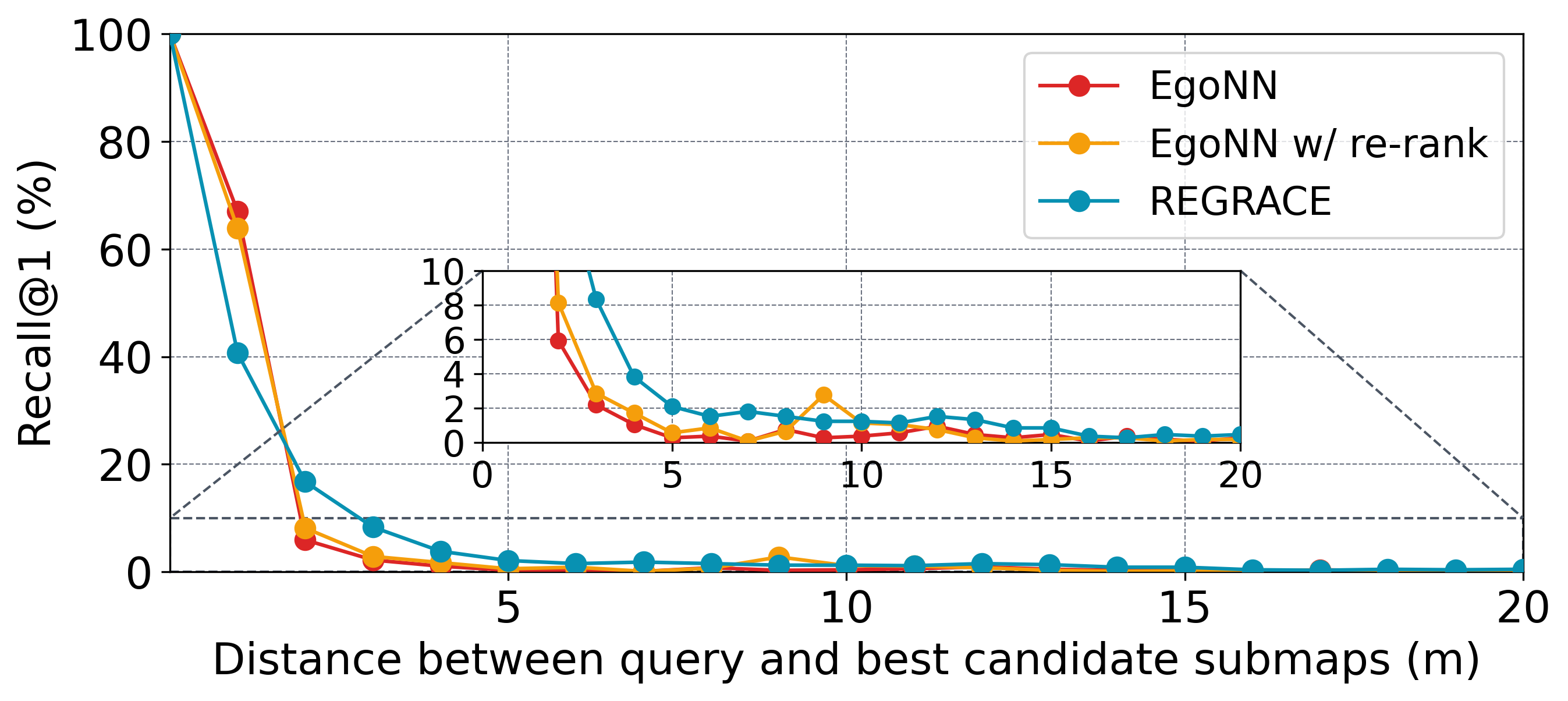
At 20 m, REGRACE’s sequence 00/08 Recall@1 values are 87.2/89.6 and maximum F1 values 90.8/85.2. These exceed the original EgoNN rows and also its consistency-enhanced maximum F1 values 87.7/80.7. EgoNN remains stronger on several 5 m retrieval metrics, particularly reverse-loop sequence 08. The original SGPR paper’s restricted candidate-pair results are separately marked and are not comparable to exhaustive database querying.
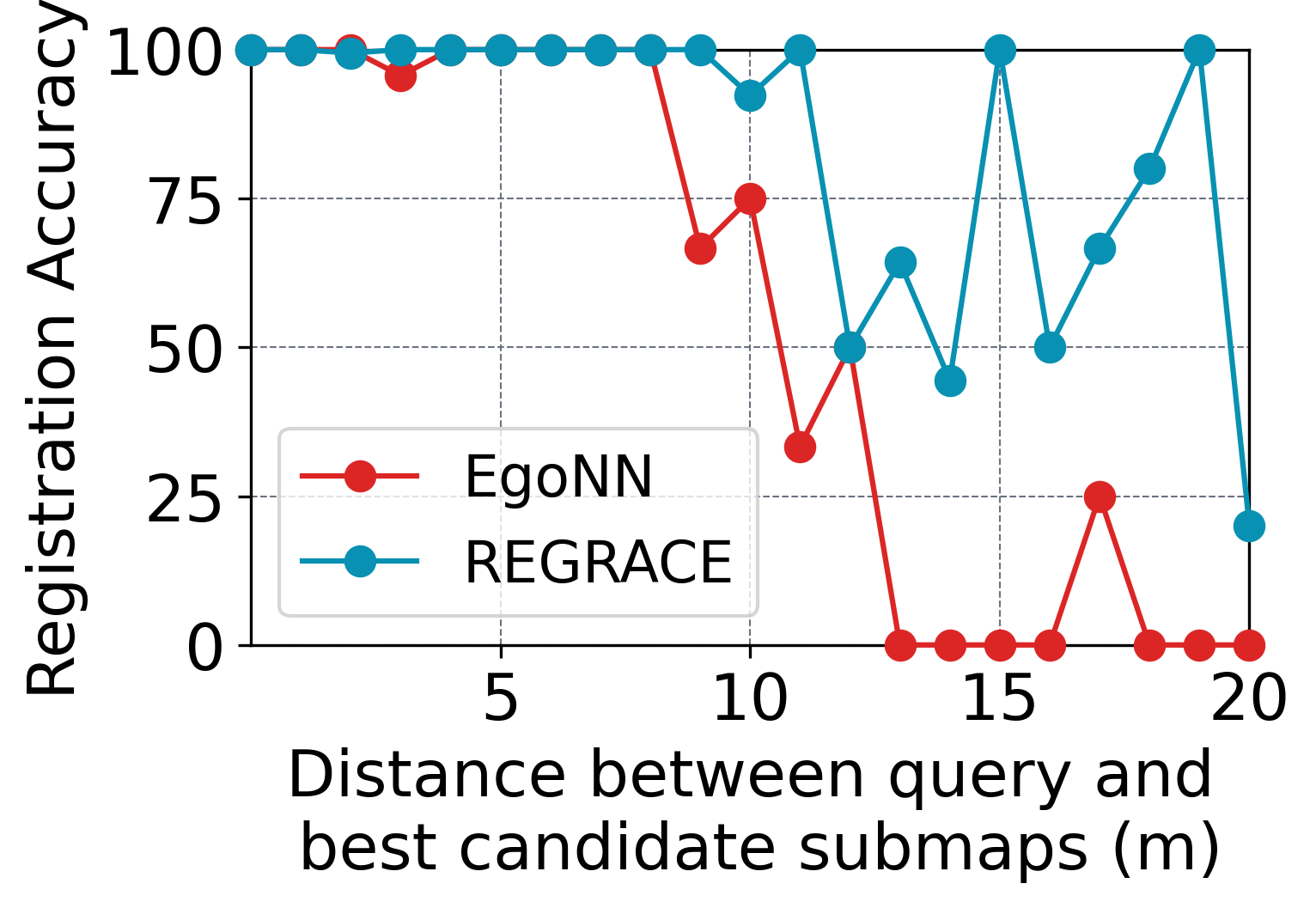
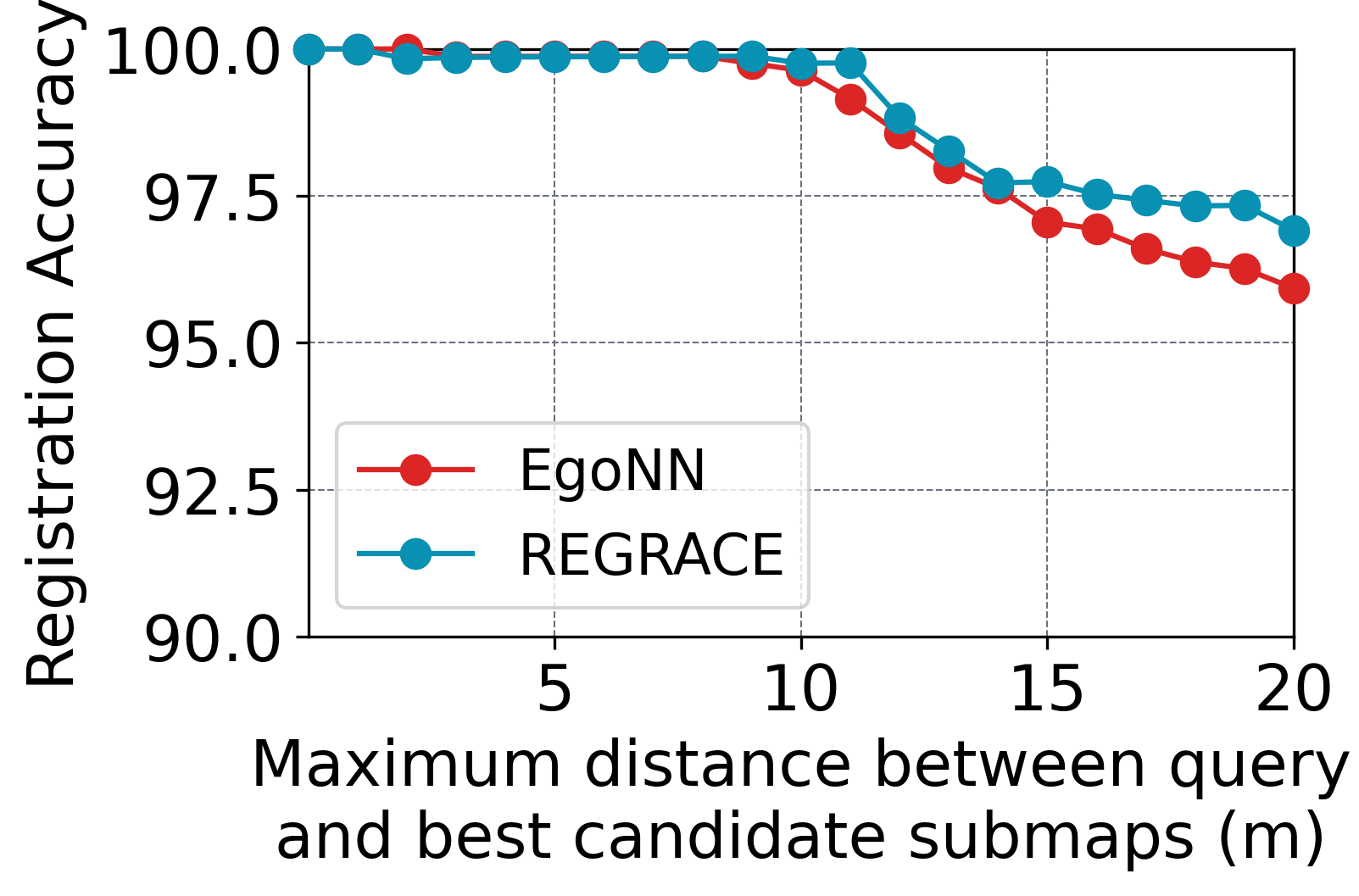
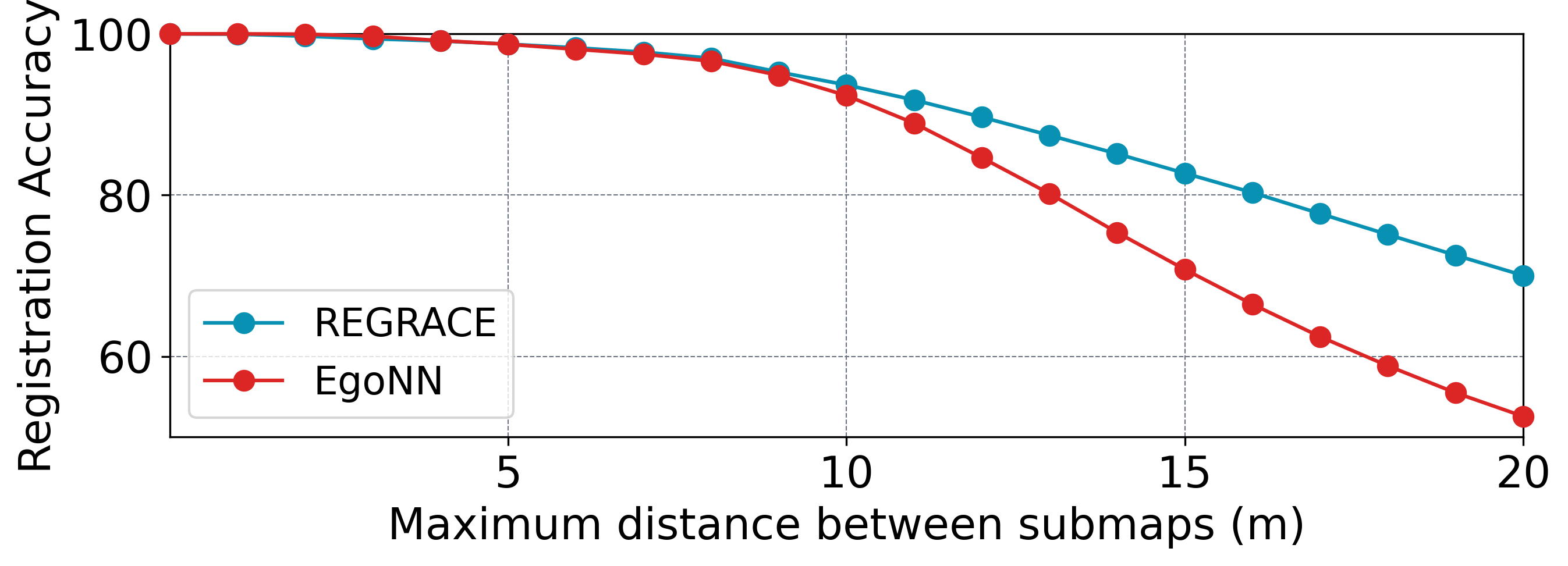
Registration succeeds 70.1% versus EgoNN52.3% on sequence 00, a 17.8-point increase; on 08 it succeeds 69.7% versus 72.4%. Among successes, REGRACE has lower mean translation/rotation errors in both sequences: 5.33 cm/0.21° and 9.04 cm/0.48°. These conditional errors do not imply uniformly higher registration success.
The timing table reports 24.3 ms inference, 56.2 ms re-ranking, and 56.1 ms registration, totaling 136.6 ms, versus 329.6 ms for EgoNN—about 2.4× faster for those stages. The stated 7.5 Hz is approximate; the listed sum implies about 7.3 Hz. Semantic segmentation, scan accumulation, and clustering are not separately timed, so the table does not establish that complete online preprocessing fits within that budget.
| Method | 00 | 02 | 05 | 06 | 08 | Avg. |
|---|---|---|---|---|---|---|
| SGPR[6] | 8.8 | 23.3 | 58.6 | 63.7 | 0.1 | 30.9 |
| SGPR[6] + RR | 18.6 | 51.9 | 74.4 | 93.2 | 2.9 | 48.2 |
| SGPR[6] + RR/CE | 61.1 | 49.7 | 79.6 | 94.4 | 0.2 | 57.0 |
| EgoNN[12] | 98.1 | 89.8 | 97.8 | 99.8 | 85.1 | 94.1 |
| EgoNN[12] + RR | 97.5 | 87.7 | 95.8 | 99.8 | 82.1 | 92.6 |
| EgoNN[12] + RR/CE | 100.0 | 94.3 | 99.5 | 100.0 | 89.2 | 96.6 |
| REGRACE† | 84.6 | 82.3 | 83.8 | 100.0 | 34.7 | 77.1 |
| REGRACE (ours) | 99.2 | 88.9 | 97.8 | 100.0 | 82.6 | 93.7 |
REGRACE with re-ranking but without consistency evaluation
| Method | 00 | 08 | ||||||||||
|---|---|---|---|---|---|---|---|---|---|---|---|---|
| 5m | 20m | 5m | 20m | |||||||||
| R@1 | R@5 | R@1 | R@5 | R@1 | R@5 | R@1 | R@5 | |||||
| SGPR[6] | 53.9 | 77.6 | 11.1 | 50.3 | 73.6 | 19.0 | 3.3 | 13.9 | 1.9 | 39.1 | 69.7 | 22.2 |
| EgoNN[12] | 98.0 | 98.5 | 96.5 | 82.2 | 86.3 | 85.1 | 90.5 | 97.4 | 83.6 | 69.0 | 78.9 | 69.9 |
| REGRACE (ours) | 92.0 | 93.5 | 99.4 | 87.2 | 88.4 | 90.8 | 73.5 | 84.7 | 86.7 | 89.6 | 91.9 | 85.2 |
| Method | 00 | 08 | ||||||||||
|---|---|---|---|---|---|---|---|---|---|---|---|---|
| 5m | 20m | 5m | 20m | |||||||||
| R@1 | R@5 | R@1 | R@5 | R@1 | R@5 | R@1 | R@5 | |||||
| SGPR[6] | 53.9 | 77.6 | 11.1 | 50.3 | 73.6 | 19.0 | 3.3 | 13.9 | 1.9 | 39.1 | 69.7 | 22.2 |
| SGPR[6] + RR | 65.7 | 77.7 | 24.5 | 63.5 | 74.6 | 36.2 | 6.1 | 20.6 | 1.5 | 38.4 | 72.3 | 36.7 |
| SGPR[6] + RR/CE | 60.8 | 78.3 | 65.7 | 63.4 | 75.3 | 43.8 | 5.8 | 19.5 | 2.1 | 38.5 | 72.4 | 39.8 |
| EgoNN[12] | 98.0 | 98.5 | 96.5 | 82.2 | 86.3 | 85.1 | 90.5 | 97.4 | 83.6 | 69.0 | 78.9 | 69.9 |
| EgoNN[12] + RR | 98.8 | 99.3 | 96.1 | 86.5 | 88.3 | 84.4 | 96.6 | 99.1 | 81.5 | 83.2 | 85.0 | 69.1 |
| EgoNN[12] + RR/CE | 98.9 | 99.4 | 99.7 | 86.3 | 88.3 | 87.7 | 96.9 | 99.2 | 89.9 | 82.9 | 84.6 | 80.7 |
| REGRACE† | 91.9 | 93.4 | 83.2 | 87.2 | 88.2 | 73.2 | 71.6 | 84.4 | 42.1 | 89.1 | 91.7 | 44.1 |
| REGRACE (ours) | 92.0 | 93.5 | 99.4 | 87.2 | 88.4 | 90.8 | 73.5 | 84.7 | 86.7 | 89.6 | 91.9 | 85.2 |
REGRACE with re-ranking and without consistency evaluation
V-B Ablation Studies
Ablations use the 100-epoch network without final refinement and classify revisits by embedding distance, isolating changes from consistency evaluation. Full connectivity raises F1 from 66.7 to 71.4 relative to ten-neighbor graphs; adding the similarity loss raises it to 77.0.
The table identifies [D] as VLAD, [E] as global mean, and [F] as GeM, with F1 values 57.1,59.2, and 71.4 respectively. The surrounding prose swaps the D/E labels; the table is preserved and used here. These settings do not directly reproduce the final consistency-based scores in the main comparison.
VI CONCLUSIONS
Compact object descriptors and geometric verification give strong long-range submap matching at the measured computation cost. Results remain dependent on semantic segmentation, submap construction, overlap, and the evaluated urban dataset.
Attention pooling, local-instance consistency losses, and integration into scene-graph SLAM are proposed future work. The experiments do not yet demonstrate full-map drift correction, arbitrary environment transfer, or a complete real-time SLAM system.