At a glance
Finite object symmetries identify physically equivalent configurations without reducing configuration-space dimension. This paper adapts distance queries, sampling, local planning, and path reconstruction to the resulting quotient space. Under regularity and clearance assumptions, standard RRT/PRM bounds improve with symmetry-group order. Experiments show shorter paths and substantial runtime benefits for selected planners and resource settings, while RRT* and fixed-budget roadmaps can be slower because symmetry-aware distance computation and extra connections have a cost.
I Introduction
A cube can reach the same physical goal through several equivalent orientations; planning to one arbitrary representative can add unnecessary rotation. Unlike continuous symmetry, finite symmetry cannot simply remove a coordinate. The quotient retains dimension but changes global topology. The authors implement planning primitives directly through representatives, avoiding an explicit Euclidean embedding of that quotient. The setting includes symmetric rigid objects in two or three dimensions, antipodal quaternion equivalence, and products of independent object symmetries. The experiments concern collision-free geometric paths, not dynamic execution or contact-force planning.
II Related Work
Trajectory optimization handles many constraints directly but faces nonconvex initialization problems. RRT [20] and PRM [21] instead explore sampled collision-free configurations. Earlier symmetry methods exploit search graphs, dynamics, or goal costs; treating goal representatives as discrete decisions is another alternative. Explicit quotient embeddings exist in some cases but can complicate inversion and collision checks. This work follows the IMACS abstraction [12] so familiar sampling planners can operate through geometric primitives. Equivariant learning motivates possible sample-efficiency gains, but the presented method neither trains a model nor requires robot demonstrations.
III Background
Group actions describe which configurations are equivalent; Riemannian geometry supplies distance, geodesics, volume, and the scale at which local neighborhoods remain ordinary. These notions determine both implementation and the assumptions of the complexity analysis.
III-A Group Theory
A group has an associative composition law, identity, and inverses. Acting on configurations produces an orbit: all configurations related by the symmetry. In two dimensions, a regular n-gon has the cyclic rotation group Cₙ. Table I retains the three-dimensional finite rotation groups: cyclic, dihedral, tetrahedral, octahedral/cubic, and icosahedral/dodecahedral, with orders n, 2n, 12, 24, and 60. Reflections are not being added to SO(3).
Quaternion q and −q represent the same orientation. Multiple independently symmetric objects use a product group; two groups of sizes a and b give ab joint representatives. A cylinder also has continuous axial symmetry, which must be handled separately from its residual flip symmetry. These equivalences are valid only for the properties relevant to the task; visual marks, grasp restrictions, or unequal dynamics could distinguish otherwise identical geometric shapes.
| Group Name | Order | Examples of Corresponding Objects |
|---|---|---|
| Cyclic Group of Order | Pyramid with a regular -gon base (abbreviated as -Pyramid) | |
| Dihedral Group of Order | Prism with a regular -gon base (abbreviated as -Prism) | |
| Alternating Group on 4 Elements | Tetrahedron | |
| Symmetric Group on 4 Elements | Cube, Octahedron | |
| Alternating Group on 5 Elements | Dodecahedron, Icosahedron |
III-B Symmetry Groups Acting on Manifolds
The Riemannian metric measures curve length through Equation 1. Within the injectivity radius, sufficiently short geodesics are unique shortest paths. For the regular isometric group actions considered here, the quotient identifies each orbit while preserving local geometry and dimension. Equation 2 computes quotient distance by fixing one representative and minimizing over the other orbit. With a separable product metric, object-wise distance calculations avoid enumerating every joint representative, so cost grows linearly in object count for fixed per-object groups.
The smooth-manifold argument depends on free, proper finite isometric actions, rather than arbitrary symmetries with fixed-point singularities. Uniform sampling upstairs projects to a uniform normalized distribution downstairs, although the unnormalized total volume decreases by the group order. The local one-to-one argument used later applies below the quotient injectivity radius; one should not infer uniform local-ball sampling at arbitrary large radii merely from projection.
Equations 1–2
| (1) |
| (2) |
IV Methodology
The method first replaces the planner’s geometric operations with symmetry-aware versions, then analyzes how quotient volume and local neighborhoods change the familiar completeness and optimality bounds.
IV-A Sampling-Based Planning
Equations 3–4 distinguish a path between chosen configurations from a path between their equivalence classes. Collision freedom must be invariant under every symmetry: transforming a configuration cannot change whether it collides. For dynamic tasks, inertia, friction, and other relevant properties would also have to agree, but those extensions are not established here.
Four primitives suffice. Distance selects the closest equivalent endpoint. Global sampling draws in the original configuration space and projects to the quotient. Local sampling projects samples around a chosen representative, with the small-neighborhood conditions needed for the analysis. The local planner connects the closest representatives by a geodesic—linear interpolation for Euclidean factors and spherical interpolation for rotations [44]—then collision-checks that path. Failure of this local attempt does not prove that no longer path exists.
Implementation stores a canonical representative at each graph vertex and an edge-specific equivalent endpoint for each directed edge. Opposite directions generally need different endpoint representatives. A returned graph path cannot be concatenated naively: successive symmetry transformations must be propagated so each lifted segment starts where the previous one ends. This produces a continuous physical trajectory with the quotient path’s length, ending at a goal-equivalent configuration rather than necessarily the original numerical goal representative.
Equations 3–4
| (3) |
| (4) |
IV-B Analysis of Sampling-Based Planning Algorithms
The core volume identities divide total and collision-free volume by |G|. Small balls retain their local geometry, so a projected uniform sample has |G| times the chance of hitting an equivalent target ball. The stated injectivity-radius lower bound is the original radius divided by |G|, tight for cyclic examples. A reference path of length ℓ must have positive clearance δ smaller than the quotient injectivity radius; the projected path then retains that clearance and length.
These results improve bounds under the inherited sampling, metric, and planner assumptions. They do not guarantee fewer samples or shorter wall-clock time in every run. The original bounds return when |G| = 1. The exact lemmas, corollaries, and theorem are retained below; appendix notes give the proof structure.
Lemma 1.
.
Corollary 1.
.
Lemma 2.
(Cheeger and Ebin) Fix and . Then is a diffeomorphism onto its image [45].
Corollary 2.
Fix , . If is uniformly sampled from , then the probability .
Theorem 1.
.
Corollary 3.
If is -clear with , then is -clear in .
IV-B 1 RRT Sample Complexity
Following Kleinbort et al. [46], cover a δ-clear path using step scale ν = min(δ, η), where η is the RRT extension size. The single-ball hit probability p becomes |G|p in the quotient, while path length and the covering construction stay fixed. Equation 5 therefore strengthens the exponential term in the failure-probability bound from exp(−pk) to exp(−|G|pk). This is a probabilistic-completeness bound, not an exact runtime distribution or a prescribed fixed sample-budget reduction for RRT.
Equation 5
| (5) |
IV-B 2 PRM Sampling Complexity
The Ladd–Kavraki argument [47] bounds the expected samples until a PRM connects the endpoints using a harmonic-number covering term and the ratio of free-space volume to a small-ball volume. Only the total free-space volume changes, yielding the factor 1/|G| in Equation 6. The source’s discrete covering counts are written compactly as real-valued length/clearance ratios; reproducing the underlying proof requires the associated integer-cover conventions.
Equation 6
| (6) |
IV-B 3 PRM* Connection Radius
For Radius-PRM*, the covering balls remain within the locally unchanged geometry. Substituting the smaller free-space volume into the Karaman–Frazzoli condition [48] reduces the sufficient connection-radius scaling constant by |G|⁻¹/ᵈ, as shown in Equation 7. The dimension d itself does not shrink. This is an asymptotic sufficient condition, not proof that every finite roadmap with the smaller radius remains connected.
Equation 7
| (7) |
IV-B 4 RRT* Connection Radius
For RRT*, the paper uses the corrected optimality analysis of Solovey et al. [49]. Equation 8 retains its dependence on optimal path length c*, dimension, approximation tolerance, and auxiliary parameters. Symmetry reduces the sufficient radius coefficient by |G|⁻¹/⁽ᵈ⁺¹⁾. The guarantee is convergence toward a near-optimal solution as samples grow, subject to the stated conditions; a smaller coefficient alone need not reduce practical runtime.
Equation 8
| (8) |
V Experiments
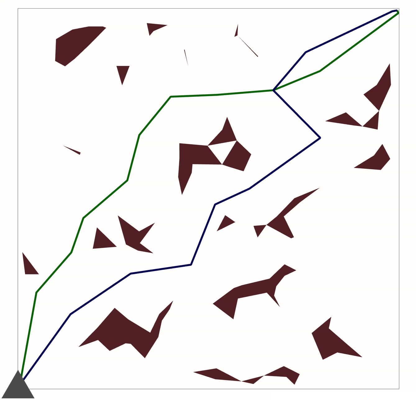
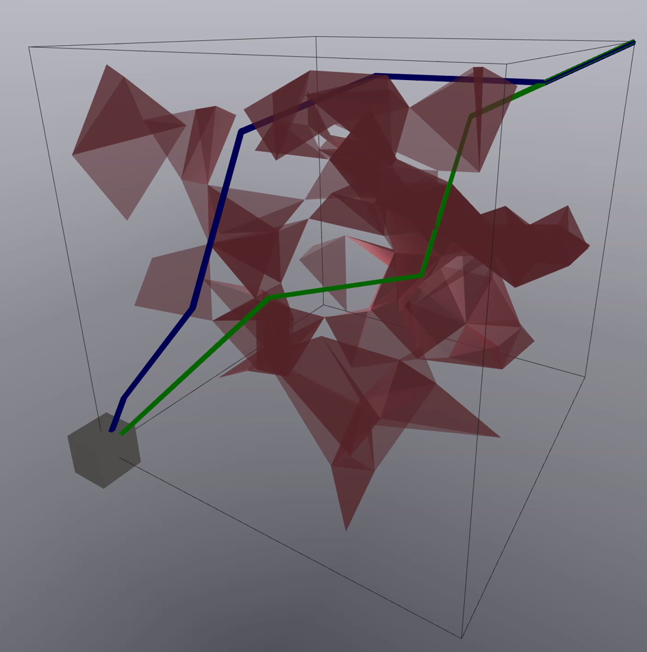
Random alpha-shape obstacle worlds [50] are tested with Drake collision checking. Each comparison uses ten worlds and 100 random start/goal pairs, evaluating RRT, RRT*, KNN-PRM*, and Radius-PRM*. Baselines plan between arbitrary fixed representatives. That comparison measures the benefit of exploiting all equivalent goals, not performance against a separate baseline that already searches every goal representative. Figures 1–2 retain the planar triangle and spatial cube examples.
For equal sampling budgets, RRT/RRT* are capped at 1,000 samples in 2D and 250 in 3D; roadmaps use 3,000|G| and 500|G| samples. Equal budgets do not mean equal wall-clock work. Table II reports baseline time or length divided by symmetry-aware time or length: values above one are improvements. RRT is roughly 2.02–2.95 times faster in the listed cases. For the cube, the path-length ratio 1.364 means about 26.7% shorter, not 36.4% shorter. RRT* is slower despite shorter paths, and cube KNN-PRM* has a 0.100 runtime ratio, meaning roughly ten times the offline construction time.
Table III applies the theoretical resource reductions: roadmap sample counts shrink by |G|, and Radius-PRM*/RRT* connection radii shrink by their derived factors. KNN neighborhood size cannot shrink because its condition depends only on dimension. Cube roadmap speedups reach 16.216 for KNN-PRM* and 32.496 for Radius-PRM*, while RRT* remains slower at 0.749. Some reduced-resource paths are longer, such as the 8-pyramid Radius-PRM* ratio 0.903. RRT is omitted because the paper does not derive a corresponding budgeting rule.
Failures are excluded from the reported averages; the authors attribute many to disconnected free space and say failure rates are similar. The PDF tables do not provide those rates or uncertainty values, instead linking complete results on the project page. The authors also estimate the unknown optimal path length in the RRT* radius using a found RRT path, so that implementation is a practical bound choice rather than access to the true optimum.
For multiple rectangles, BiRRT is capped at 40,000 samples. Table IV covers one through five objects, dimensions 3 through 15, and group orders 2 through 32. Runtime improvement rises from 1.121 to 2.747, with modest path reductions. Product symmetry improves constants while the sample requirement still grows exponentially with dimension; the experiment does not remove the curse of dimensionality.
| Workspace Dimension | Object | Symmetry Group Order | RRT Online Runtime Improvement | RRT Path Length Improvement | RRT* Online Runtime Improvement | RRT* Path Length Improvement | KNN-PRM* Offline Runtime Improvement | KNN-PRM* Path Length Improvement |
| 2 | Triangle | 3 | 2.766x | 1.216x | 0.828x | 1.133x | 0.832x | 1.069x |
| 2 | Pentagon | 5 | 2.432x | 1.187x | 0.718x | 1.141x | 0.614x | 1.107x |
| 2 | Octagon | 8 | 2.192x | 1.227x | 0.611x | 1.157x | 0.367x | 1.116x |
| 3 | 8-Pyramid | 8 | 2.016x | 1.179x | 0.844x | 1.091x | 0.347x | 1.157x |
| 3 | 6-Prism | 12 | 2.951x | 1.279x | 0.779x | 1.146x | 0.233x | 1.190x |
| 3 | Tetrahedron | 12 | 2.360x | 1.310x | 0.751x | 1.163x | 0.227x | 1.193x |
| 3 | Cube | 24 | 2.759x | 1.364x | 0.749x | 1.198x | 0.100x | 1.196x |
| Workspace Dimension | Object | Symmetry Group Order | RRT* Online Runtime Improvement | RRT* Path Length Improvement | KNN-PRM* Offline Runtime Improvement | KNN-PRM* Path Length Improvement | Radius-PRM* Offline Runtime Improvement | Radius-PRM* Path Length Improvement |
| 2 | Triangle | 3 | 0.845x | 1.133x | 3.005x | 0.992x | 2.519x | 1.003x |
| 2 | Pentagon | 5 | 0.744x | 1.141x | 5.103x | 1.002x | 7.414x | 1.090x |
| 2 | Octagon | 8 | 0.640x | 1.157x | 6.570x | 1.031x | 15.225x | 1.086x |
| 3 | 8-Pyramid | 8 | 0.845x | 1.091x | 7.057x | 1.058x | 15.776x | 0.903x |
| 3 | 6-Prism | 12 | 0.777x | 1.146x | 9.849x | 1.092x | 20.577x | 0.989x |
| 3 | Tetrahedron | 12 | 0.751x | 1.163x | 10.276x | 1.138x | 20.501x | 1.032x |
| 3 | Cube | 24 | 0.749x | 1.198x | 16.216x | 1.125x | 32.496x | 1.029x |
VI Discussion
Finite symmetry can be incorporated through representative-aware geometric primitives without explicitly embedding the quotient. The strongest practical evidence is faster RRT and reduced-resource roadmap construction, with shorter paths in many settings. Runtime gains are planner-dependent, and bounds require regular symmetry actions and sufficiently clear paths. Other planners, kinodynamic planning, trajectory optimization, hybrid methods, and Graphs of Convex Sets are suggested extensions rather than demonstrated outcomes.
| Number of Objects | Configuration Space Dimension | Symmetry Group Order | BiRRT Online Runtime Improvement | BiRRT Path Length Improvement |
| 1 | 3 | 2 | 1.121x | 1.064x |
| 2 | 6 | 4 | 1.350x | 1.099x |
| 3 | 9 | 8 | 1.824x | 1.131x |
| 4 | 12 | 16 | 2.573x | 1.137x |
| 5 | 15 | 32 | 2.747x | 1.101x |
VII Acknowledgements
The authors acknowledge colleagues, MIT SuperCloud and Lincoln Laboratory computing resources, Amazon support, and an NSF Graduate Research Fellowship, with the usual statement that findings need not represent NSF views.
Appendix: volume and local geometry
For Lemma 1, choose neighborhoods with disjoint symmetry translates, project them to cover the quotient, and partition that cover into disjoint measurable pieces Vᵢ. Each piece has |G| isometric lifts, so summing their volumes proves the factor 1/|G|. Intersecting the pieces with collision-free classes proves Corollary 1. The written proof uses a finite subcover via compactness; bounded planning regions and the relevant measure assumptions must be respected when applying it. The two displayed partition/volume identities remain intact.
The note on Lemma 2 invokes the normal-coordinate construction of Cheeger and Ebin [45]: below the injectivity radius the projection is locally invertible. This is the local geometric fact used in the ball-probability and clearance arguments.
Equations
Proof of Theorem 1
Lemma 3 uses isometries to show successive points in a symmetry orbit have equal neighbor distances: translating a shortest geodesic preserves its length, and a shorter translated path would contradict minimality. Lemma 4 then argues by contradiction along the relevant one-parameter subgroup. If distinct representatives were closer than twice the original injectivity radius divided by |G|, repeating the segment through the finite group order would create a geodesic loop shorter than the allowed minimum. Lagrange’s theorem closes that loop.
For Theorem 1, suppose two distinct short quotient geodesics violate the proposed radius bound. Lift them from the same representative. Their endpoints cannot coincide without contradicting the original injectivity radius; if distinct, Lemma 4 forces them apart. The triangle inequality in Equation 9 instead puts them closer than that separation, producing a contradiction. This proof relies on the isometric group/one-parameter-geodesic structure used by the paper; it is not a blanket claim for every quotient with singularities or every arbitrary metric.
Lemma 3.
.
Lemma 4.
, distinct, .
Equations 9
| (9) |