Literature
Display
← All papers

RAMEN: Real-time Asynchronous Multi-agent Neural Implicit Mapping

Hongrui Zhao · Boris Ivanovic · Negar Mehr

· Robotics: Science and Systems 2025 ↗

Robotics6 min text · CondensedOriginal paper ↗
Contents

Overview

The opening figure shows the two-robot hardware arrangement and complete original map comparisons, restored from the PDF.
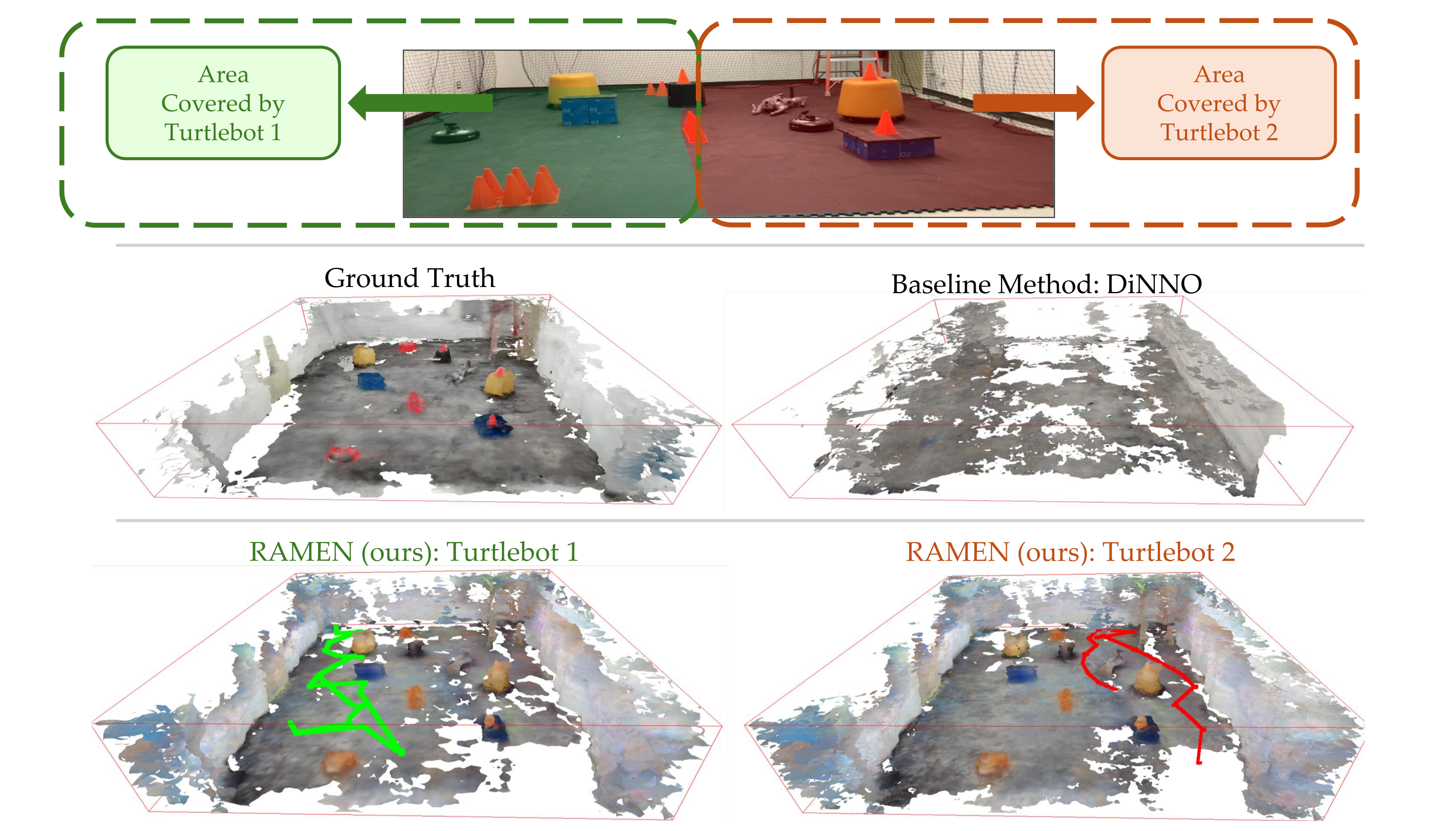
Complete original Figure 1 hardware experiment and map comparison, restored from PDF page 1.
Fig. 1: In a challenging real-world experiment with limited communication (agents can only exchange information every 30 seconds), our method RAMEN enables each turtlebot to successfully map the full scene while only physically visiting half of the scene (explored areas and trajectories are colored accordingly). Our method achieves accuracy comparable to the ground truth while the baseline method (DiNNO) fails to converge.

At a glance

RAMEN learns decentralized neural scene maps when neighboring agents exchange updates intermittently. A weighted consensus optimizer favors feature-grid parameters with more reconstruction updates, reducing the influence of poorly observed regions in stale neighbor models. Dataset experiments show better reconstruction than the tested distributed baselines under message loss, and two physical robots share maps every thirty seconds. The implementation assumes known camera poses and uses external computers; it is a mapping study rather than a complete autonomous localization-and-exploration system.

I Introduction

Sharing neural map parameters can spread observations without transmitting all raw images between mapping agents, but stale parameters can damage consensus optimization. RAMEN assigns reliability weights per feature-grid parameter instead of pausing every agent until fresh messages arrive. The goal is to retain useful older information while reducing influence from poorly learned regions. The experiments test finite delays and disruptions, not guaranteed agreement under permanent disconnection.

II Related Works

The scene representation builds on Co-SLAM [24] and multiresolution neural grids. Existing distributed neural-mapping methods, including DiNNO [13], motivate consensus optimization and provide baselines. Parameter-frequency weighting offers a low-cost alternative to ensembles or Bayesian uncertainty models, with less expressive uncertainty estimates.

The paper primarily studies message drops, with heterogeneous computation also present in the hardware demonstration. Its advantages are established against the selected optimizer implementations, not every asynchronous distributed-learning algorithm.

III Preliminaries

The preliminaries introduce the neural map and the synchronous decentralized optimization problem before deriving the weighted variant.

III-A Single-agent Neural Implicit Mapping

A multiresolution hash grid [38] encodes spatial features. Geometry and color decoders predict signed distance and color, from which RGB and depth images are rendered along known camera rays. Reconstruction losses supervise observed color, depth, signed distance, free space, and geometric smoothness.

RAMEN later fixes the decoders and optimizes the feature grid only. Thus these equations describe the underlying representation, while the actual distributed parameters differ from a fully trainable Co-SLAM model.

Equations 1–5
Fτ​(γ⁡(𝐱),Vα​(𝐱))→(𝐡,s).F_{\tau}\left(\gamma(\mathbf{x}),V_{\alpha}(\mathbf{x})\right)\to(\mathbf{h},s). (1)
OPENFϕ​(γ⁡(𝐱),𝐡))→𝐜.F_{\phi}\left(\gamma(\mathbf{x}),\mathbf{h})\right)\to\mathbf{c}. (2)
𝐜^=1∑i=1Mwi​∑i=1Mwi​𝐜i,\displaystyle\hat{\mathbf{c}}=\frac{1}{\sum^{M}_{i=1}w_{i}}\sum_{i=1}^{M}w_{i}\mathbf{c}_{i}, (3a)
d^=1∑i=1Mwi​∑i=1Mwi​𝐝i,\displaystyle\hat{d}=\frac{1}{\sum^{M}_{i=1}w_{i}}\sum_{i=1}^{M}w_{i}\mathbf{d}_{i}, (3b)
wi=σ⁡(sit​r)​σ​(−sit​r).w_{i}=\sigma\left(\frac{s_{i}}{tr}\right)\sigma\left(-\frac{s_{i}}{tr}\right). (4)
Lo​b​j​(𝚯,R)=Lr​g​b+Ld+Ls​d​f+Lf​s+Ls​m​o​o​t​h,L^{obj}(\mathbf{\Theta},R)=L_{rgb}+L_{d}+L_{sdf}+L_{fs}+L_{smooth}, (5)

III-B Synchronous Multi-agent Mapping

Each robot minimizes reconstruction loss on its posed RGBD images while matching neighboring parameter vectors. Auxiliary edge variables and dual variables express local consensus without a central fusion variable. Alternating-direction optimization [42] yields primal map updates and dual disagreement updates; in practice, a few stochastic-gradient steps approximate each primal minimization.

The synchronous formulation assumes current neighbor states are available. An old copy can conflict with newly observed geometry, motivating per-parameter weighting rather than indiscriminate agreement.

Equations 6–9b
Lio​b​j​(𝚯i,Ri)=Lr​g​bi+Ldi+Ls​d​fi+Lf​si+Ls​m​o​o​t​hi,L^{obj}_{i}(\mathbf{\Theta}_{i},R_{i})={L_{rgb}}_{i}+{L_{d}}_{i}+{L_{sdf}}_{i}+{L_{fs}}_{i}+{L_{smooth}}_{i}, (6)
min⁡∑i∈𝒱{𝚯1,⋯}​{𝐳i​j,⋯}⁡Lio​b​j​(𝚯i,Ri),\displaystyle\min_{\{\mathbf{\Theta}_{1},\cdots\}\{\mathbf{z}_{ij},\cdots\}}\;\sum_{i\in\mathcal{V}}L^{obj}_{i}(\mathbf{\Theta}_{i},R_{i}), (7a)
s.t.​𝚯i=𝐳i​j,𝚯j=𝐳i​j,∀(i,j)∈ℰ,\displaystyle\text{s.t.}\;\mathbf{\Theta}_{i}=\mathbf{z}_{ij},\mathbf{\Theta}_{j}=\mathbf{z}_{ij},\;\forall(i,j)\in\mathcal{E}, (7b)
ℒa=∑i∈𝒱(Lio​b​j​(𝚯i,Ri)+∑j∈Ni𝝀i​j⊤​(𝚯i−𝐳i​j)CLOSE\displaystyle\mathcal{L}^{a}=\sum_{i\in\mathcal{V}}\Bigg(L^{obj}_{i}(\mathbf{\Theta}_{i},R_{i})+\sum_{j\in N_{i}}\boldsymbol{\lambda}_{ij}^{\top}(\mathbf{\Theta}_{i}-\mathbf{z}_{ij})
OPEN+𝐯i​j⊤​(𝚯j−𝐳i​j)+ρ2​‖𝚯i−𝐳i​j‖22+ρ2​‖𝚯j−𝐳i​j‖22),\displaystyle+\mathbf{v}_{ij}^{\top}(\mathbf{\Theta}_{j}-\mathbf{z}_{ij})+\frac{\rho}{2}\|\mathbf{\Theta}_{i}-\mathbf{z}_{ij}\|_{2}^{2}+\frac{\rho}{2}\|\mathbf{\Theta}_{j}-\mathbf{z}_{ij}\|_{2}^{2}\Bigg), (8)
𝚯it+1=\displaystyle\mathbf{\Theta}_{i}^{t+1}= argmin𝚯iLio​b​j​(𝚯i,Ri)+𝚯i⊤​𝐩it\displaystyle\operatornamewithlimits{argmin}_{\mathbf{\Theta}_{i}}\;L^{obj}_{i}(\mathbf{\Theta}_{i},R_{i})+\mathbf{\Theta}_{i}^{\top}\mathbf{p}_{i}^{t}
+ρ∑j∈Ni‖𝚯i−𝚯it+𝚯jt2‖22,\displaystyle+\rho\sum_{j\in N_{i}}\left\|\mathbf{\Theta}_{i}-\frac{\mathbf{\Theta}_{i}^{t}+\mathbf{\Theta}_{j}^{t}}{2}\right\|_{2}^{2}, (9a)
𝐩it+1=\displaystyle\mathbf{p}_{i}^{t+1}= 𝐩it+ρ​∑j∈Ni(𝚯it+1−𝚯jt+1).\displaystyle\mathbf{p}_{i}^{t}+\rho\sum_{j\in N_{i}}(\mathbf{\Theta}_{i}^{t+1}-\mathbf{\Theta}_{j}^{t+1}). (9b)

IV Asynchronous Multi-agent Neural Implicit Mapping

The proposed method combines a weighted decentralized optimizer with an update-frequency reliability heuristic. It permits local mapping to continue when neighbor updates are missing.

IV-A Uncertainty-Weighted Decentralized C-ADMM

Each edge assigns diagonal weights to the two agents’ parameter vectors. The auxiliary consensus target becomes their reliability-weighted average; primal and dual updates penalize departure from that target. This allows a robot to retain information from a neighbor about regions it has not itself visited, while reducing influence from weakly updated neighbor parameters.

The retained derivation gives the weighted update rules. It is not a convergence proof for arbitrary nonconvex neural maps, stochastic approximate solves, time-varying weights, or unbounded message loss. Those behaviors are evaluated empirically in the reported settings.

Equations 10–14
ℒw​a=∑i∈𝒱(Lio​b​j​(𝚯i,Ri)+∑j∈Ni𝝀i​j⊤​(𝚯i−𝐳i​j)CLOSE\displaystyle\mathcal{L}^{wa}=\sum_{i\in\mathcal{V}}\Bigg(L^{obj}_{i}(\mathbf{\Theta}_{i},R_{i})+\sum_{j\in N_{i}}\boldsymbol{\lambda}_{ij}^{\top}(\mathbf{\Theta}_{i}-\mathbf{z}_{ij})
OPEN+𝐯i​j⊤​(𝚯j−𝐳i​j)+ρ2​‖𝚯i−𝐳i​j‖𝐖i​j2+ρ2​‖𝚯j−𝐳i​j‖𝐖j​i2),\displaystyle+\mathbf{v}_{ij}^{\top}(\mathbf{\Theta}_{j}-\mathbf{z}_{ij})+\frac{\rho}{2}\|\mathbf{\Theta}_{i}-\mathbf{z}_{ij}\|_{\mathbf{W}_{ij}}^{2}+\frac{\rho}{2}\|\mathbf{\Theta}_{j}-\mathbf{z}_{ij}\|_{\mathbf{W}_{ji}}^{2}\Bigg), (10)
𝐳i​jt+1=(𝐖i​jt+𝐖j​it)−1​(𝐖i​jt​𝚯it+𝐖j​it​𝚯jt)\displaystyle\mathbf{z}_{ij}^{t+1}=(\mathbf{W}_{ij}^{t}+\mathbf{W}_{ji}^{t})^{-1}(\mathbf{W}_{ij}^{t}\mathbf{\Theta}_{i}^{t}+\mathbf{W}_{ji}^{t}\mathbf{\Theta}_{j}^{t})
+1ρ​(𝐖i​jt+𝐖j​it)−1​(𝝀i​jt+𝐯i​jt).\displaystyle\hskip 42.67912pt+\frac{1}{\rho}(\mathbf{W}_{ij}^{t}+\mathbf{W}_{ji}^{t})^{-1}(\boldsymbol{\lambda}_{ij}^{t}+\mathbf{v}_{ij}^{t}). (11)
𝝀i​jt+1=𝝀i​jt+ρ​𝐖i​jt​∇𝝀i​jℒw​a,\displaystyle\boldsymbol{\lambda}_{ij}^{t+1}=\boldsymbol{\lambda}_{ij}^{t}+\rho\mathbf{W}_{ij}^{t}\nabla_{\boldsymbol{\lambda}_{ij}}\mathcal{L}^{wa}, (12a)
𝐯i​jt+1=𝐯i​jt+ρ​𝐖j​it​∇𝐯i​jℒw​a,\displaystyle\mathbf{v}_{ij}^{t+1}=\mathbf{v}_{ij}^{t}+\rho\mathbf{W}_{ji}^{t}\nabla_{\mathbf{v}_{ij}}\mathcal{L}^{wa}, (12b)
∇𝝀i​jℒw​a=𝚯it+1−𝐳i​jt+1,\displaystyle\nabla_{\boldsymbol{\lambda}_{ij}}\mathcal{L}^{wa}=\mathbf{\Theta}_{i}^{t+1}-\mathbf{z}_{ij}^{t+1}, (13a)
∇𝐯i​jℒw​a=𝚯jt+1−𝐳i​jt+1,\displaystyle\nabla_{\mathbf{v}_{ij}}\mathcal{L}^{wa}=\mathbf{\Theta}_{j}^{t+1}-\mathbf{z}_{ij}^{t+1}, (13b)
𝐳i​jt+1=(𝐖i​jt+𝐖j​it)−1​(𝐖i​jt​𝚯it+𝐖j​it​𝚯jt),\mathbf{z}_{ij}^{t+1}=(\mathbf{W}_{ij}^{t}+\mathbf{W}_{ji}^{t})^{-1}(\mathbf{W}_{ij}^{t}\mathbf{\Theta}_{i}^{t}+\mathbf{W}_{ji}^{t}\mathbf{\Theta}_{j}^{t}), (14)

Refer to caption

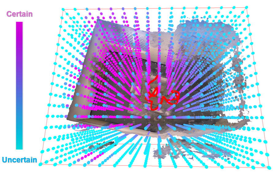
Fig. 2: This visualization shows the uncertainty associated with the parameters in the coarsest feature grid Vαl=1V_{\alpha}^{l=1} of the neural implicit map. We represent this uncertainty by overlaying color-coded vertices on the reconstructed 3D mesh. The robot’s trajectory is shown in red. The robot’s trajectory and field-of-view are limited to the left half of the room. As expected, high uncertainty (blue vertices) corresponds to the right half of the map not explored by the robot where the reconstructed geometry is inaccurate.
Equations 15–17
𝚯it+1=argmin𝚯iLio​b​j​(𝚯i,Ri)+∑j∈Ni2​𝚯i⊤​𝝀i​jt\displaystyle\mathbf{\Theta}_{i}^{t+1}=\operatornamewithlimits{argmin}_{\mathbf{\Theta}_{i}}\;L^{obj}_{i}(\mathbf{\Theta}_{i},R_{i})+\sum_{j\in N_{i}}2\mathbf{\Theta}_{i}^{\top}\boldsymbol{\lambda}_{ij}^{t}
+ρ​‖𝚯i−(𝐖i​jt+𝐖j​it)−1​(𝐖i​jt​𝚯it+𝐖j​it​𝚯jt)‖𝐖i​jt2,\displaystyle+\rho\|\mathbf{\Theta}_{i}-(\mathbf{W}_{ij}^{t}+\mathbf{W}_{ji}^{t})^{-1}(\mathbf{W}_{ij}^{t}\mathbf{\Theta}_{i}^{t}+\mathbf{W}_{ji}^{t}\mathbf{\Theta}_{j}^{t})\|_{\mathbf{W}_{ij}^{t}}^{2}, (15)
𝚯it+1=argmin𝚯iLio​b​j​(𝚯i,Ri)+𝚯i⊤​𝐩it\displaystyle\mathbf{\Theta}_{i}^{t+1}=\operatornamewithlimits{argmin}_{\mathbf{\Theta}_{i}}\;L^{obj}_{i}(\mathbf{\Theta}_{i},R_{i})+\mathbf{\Theta}_{i}^{\top}\mathbf{p}_{i}^{t}
+ρ∑j∈Ni∥𝚯i−(𝐖i​jt+𝐖j​it)−1(𝐖i​jt𝚯it+𝐖j​it𝚯jt)∥𝐖i​jt2,\displaystyle+\rho\sum_{j\in N_{i}}\|\mathbf{\Theta}_{i}-(\mathbf{W}_{ij}^{t}+\mathbf{W}_{ji}^{t})^{-1}(\mathbf{W}_{ij}^{t}\mathbf{\Theta}_{i}^{t}+\mathbf{W}_{ji}^{t}\mathbf{\Theta}_{j}^{t})\|_{\mathbf{W}_{ij}^{t}}^{2}, (16)
𝐩it+1=𝐩it+\displaystyle\mathbf{p}_{i}^{t+1}=\mathbf{p}_{i}^{t}+
2​ρ​𝐖i​jt​∑j∈Ni(𝐖i​jt+𝐖j​it)−1​(𝐖j​it​𝚯it+1−𝐖j​it​𝚯jt+1),\displaystyle 2\rho\mathbf{W}_{ij}^{t}\sum_{j\in N_{i}}(\mathbf{W}_{ij}^{t}+\mathbf{W}_{ji}^{t})^{-1}(\mathbf{W}_{ji}^{t}\mathbf{\Theta}_{i}^{t+1}-\mathbf{W}_{ji}^{t}\mathbf{\Theta}_{j}^{t+1}), (17)

Refer to caption

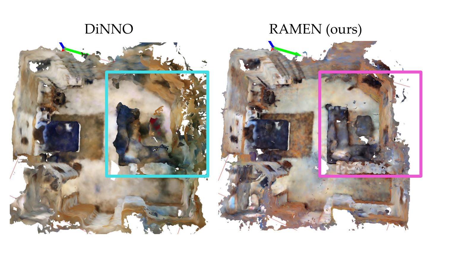
Fig. 3: Comparison of scene reconstructions from DiNNO and RAMEN (ours) on ScanNet “scene0000” with only 50% communication success rate. RAMEN produces more accurate and detailed geometry in the highlighted region.

IV-B Frequency-based Epistemic Uncertainty

The reliability statistic counts nonzero reconstruction-gradient updates for each grid parameter. More updates are interpreted as better observation coverage and lower uncertainty. The geometry and color decoders are pretrained on the NICE-SLAM apartment data and frozen, avoiding the harder problem of assigning spatial reliability to shared decoder weights. Agents also share the same map initialization.

Neighbor count vectors are jointly scaled into user-selected lower and upper weight bounds, preserving their relative magnitudes. This is a frequency heuristic, not a calibrated posterior variance. Old neighbor counts lag behind continued local learning; the stated equation does not separately estimate uncertainty from elapsed wall-clock age. Replayed observations can add updates without supplying independent new viewpoints.

Algorithm 1 retains the complete capture, communication, local-gradient, dual-update, and reliability-update loop. Only feature-grid parameters and their statistics enter the consensus exchange.

Equation 18
𝐮it=∑k=0tsgn​(abs​(∂Li,ko​b​j∂𝚯ik)),\mathbf{u}_{i}^{t}=\sum_{k=0}^{t}\text{sgn}\left(\text{abs}\left(\frac{\partial L^{obj}_{i,k}}{\partial\mathbf{\Theta}_{i}^{k}}\right)\right), (18)
Algorithm 1 RAMEN: Real-time Asynchronous Multi-agent Neural Implicit Mapping
1: for i∈𝒱i\in\mathcal{V} do
2:   𝐩i0=0\mathbf{p}_{i}^{0}=0
3:   𝚯i0=𝚯initial\mathbf{\Theta}_{i}^{0}=\mathbf{\Theta}_{\text{initial}}
4: end for
5: while true do
6:   for i∈𝒱i\in\mathcal{V} do
7:    Capture images and add to database RiR_{i}
8:    Send 𝚯it\mathbf{\Theta}_{i}^{t} and 𝐮it\mathbf{u}_{i}^{t} to neighbors NiN_{i}
9:   end for
10:   for i∈𝒱i\in\mathcal{V} do
11:    Compute (19) to get 𝐖i​jt,𝐖j​it\mathbf{W}_{ij}^{t},\mathbf{W}_{ji}^{t}
12:    for b←0​to​Bb\leftarrow 0\;\text{to}\;B do
13:      Sample from RiR_{i}
14:      Gradient descent on (16) to approximate 𝚯it+1\mathbf{\Theta}_{i}^{t+1}
15:    end for
16:    Perform dual variable update (17) to obtain 𝐩it+1\mathbf{p}_{i}^{t+1}
17:    Compute (18) to get 𝐮it+1\mathbf{u}_{i}^{t+1}
18:   end for
19: end while
Equations 19a–19d
𝐮s​u​m:=𝐮iti+𝐮jtj,\displaystyle\mathbf{u}_{sum}:=\mathbf{u}_{i}^{t_{i}}+\mathbf{u}_{j}^{t_{j}}, (19a)
ϵ=βu−βlmax​(𝐮s​u​m)−min​(𝐮s​u​m),\displaystyle\epsilon=\frac{\beta_{u}-\beta_{l}}{\text{max}(\mathbf{u}_{sum})-\text{min}(\mathbf{u}_{sum})}, (19b)
ζ=βl−ϵ⋅min​(𝐮s​u​m),\displaystyle\zeta=\beta_{l}-\epsilon\cdot\text{min}(\mathbf{u}_{sum}), (19c)
𝐖i​j=diag​(ϵ⋅𝐮iti+ζ),𝐖j​i=diag​(ϵ⋅𝐮jtj+ζ),\displaystyle\mathbf{W}_{ij}=\text{diag}(\epsilon\cdot\mathbf{u}_{i}^{t_{i}}+\zeta),\mathbf{W}_{ji}=\text{diag}(\epsilon\cdot\mathbf{u}_{j}^{t_{j}}+\zeta), (19d)

V Results

Evaluation uses posed RGBD streams from synthetic Replica and real ScanNet scenes, simulated communication disruption, and a two-robot experiment. Meshes are extracted from the learned fields. “Artifacts” measures reconstructed-to-reference distance, while “holes” measures reference-to-reconstructed distance. Completion uses a five-centimetre proximity threshold; the paper’s wording about which point set defines its percentage is imprecise, so the original metric label and reported numbers are retained rather than silently redefining it.

TABLE I: RAMEN significantly outperforms prior state-of-the-art approaches for multi-agent neural implicit mapping in challenging communication conditions.
Method Metric office1 room1 scene0000 scene0106 Avg.
DSGD Artifacts (cm) ↓\downarrow 6.38±\pm1.76 16.39±\pm0.45 14.59±\pm0.57 100.40±\pm5.02 34.34±\pm1.95
Holes (cm) ↓\downarrow 2.70±\pm0.20 2.55±\pm0.02 5.03±\pm0.16 6.35±\pm0.44 4.20±\pm0.21
Completion Ratio (%) ↑\uparrow 87.21±\pm0.96 90.56±\pm0.22 74.34±\pm0.82 65.01±\pm1.61 79.03±\pm0.90
DSGT Artifacts (cm) ↓\downarrow 20.76±\pm8.31 17.66±\pm1.92 N/A N/A N/A
Holes (cm) ↓\downarrow 9.09±\pm6.28 2.58±\pm0.05 N/A N/A N/A
Completion Ratio (%) ↑\uparrow 56.47±\pm1.30 90.69±\pm0.41 N/A N/A N/A
DiNNO Artifacts (cm) ↓\downarrow 2.78±\pm0.34 5.78±\pm1.50 7.56±\pm2.62 61.29±\pm7.41 19.35±\pm2.97
Holes (cm) ↓\downarrow 2.79±\pm0.22 2.33±\pm0.22 4.10±\pm0.39 5.73±\pm0.82 3.74±\pm0.41
Completion Ratio (%) ↑\uparrow 85.90±\pm2.55 91.45±\pm1.99 79.75±\pm3.71 64.73±\pm5.94 80.46±\pm3.55
RAMEN (ours) Artifacts (cm) ↓\downarrow 3.25±\pm0.35 5.47±\pm0.97 5.55±\pm0.35 37.67±\pm1.64 12.98±\pm0.83
Holes (cm) ↓\downarrow 1.78±\pm0.04 2.01±\pm0.03 3.23±\pm0.08 3.28±\pm0.11 2.57±\pm0.07
Completion Ratio (%) ↑\uparrow 94.37±\pm0.27 94.20±\pm0.32 90.72±\pm0.84 86.48±\pm0.64 91.44±\pm0.52

Refer to caption

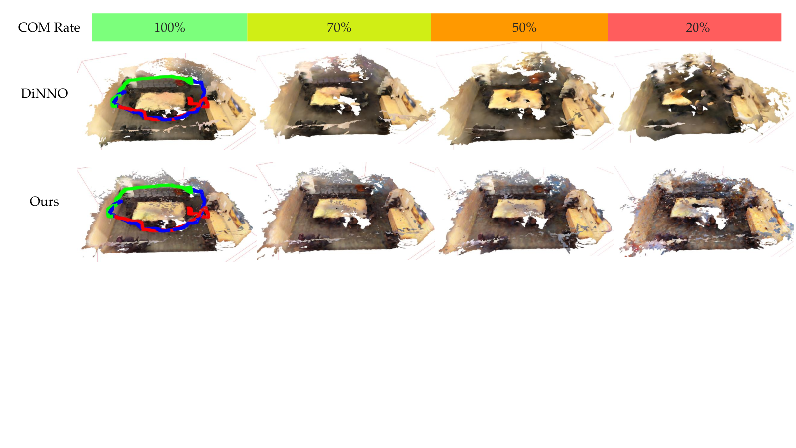
Fig. 4: Reconstruction quality of DiNNO and RAMEN (ours) on ScanNet “scene0169” under varying communication success rates (three-agent trajectories shown in different colors). Even at a 20% success rate, RAMEN preserves scene details, while DiNNO exhibits incomplete or blurry reconstructions.

Refer to caption

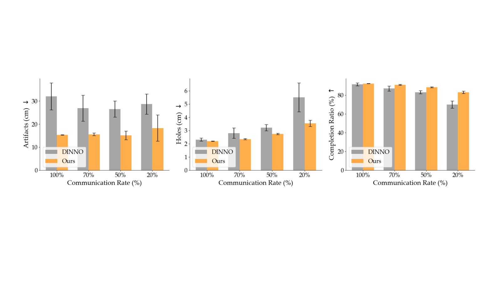
Fig. 5: Evaluation metric scores for DiNNO and RAMEN (ours) on ScanNet “scene0169” under varying communication success rates. While both methods exhibit worse scores with lower communication rate, RAMEN demonstrates greater robustness, maintaining higher accuracy and lower variance than DiNNO, especially in lower communication rates.

Refer to caption

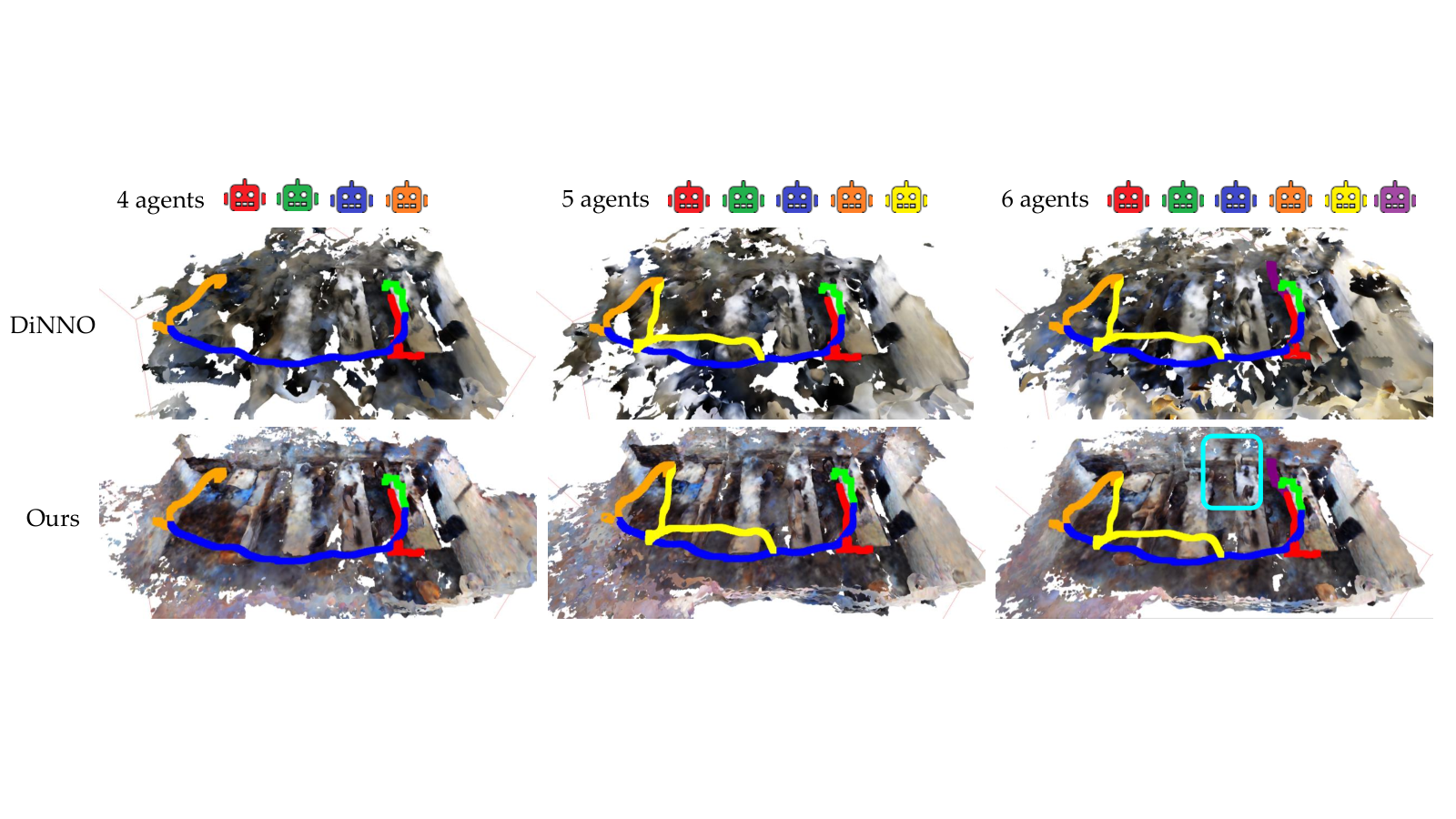
Fig. 6: Reconstruction quality of DiNNO and RAMEN (ours) on ScanNet “scene0106” with varying numbers of agents (trajectories shown in different colors). RAMEN effectively utilizes observations from additional agents to achieve a more complete scene reconstruction, particularly in the highlighted region (cyan box). In contrast, DiNNO exhibits numerous artifacts and incomplete reconstructions.

Refer to caption

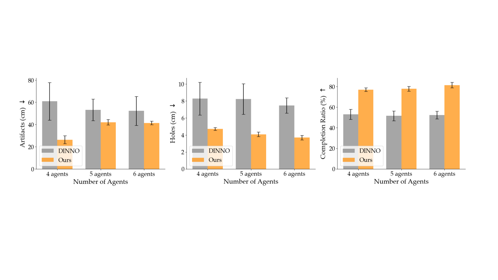
Fig. 7: Evaluation metric scores for DiNNO and RAMEN (ours) on ScanNet “scene0106” with varying numbers of agents. DiNNO exhibits worse artifact scores due to noisy reconstructions. While both methods benefit from additional agents, RAMEN more effectively leverages the increased information to achieve greater improvements in scene completion.

V-A Simulated Experiments

With three agents, a fully connected graph, and 50% message success, the four-scene average completion ratio is 91.44% for RAMEN versus 80.46% for DiNNO. Average artifact distance is 12.98 versus 19.35 cm, and hole distance 2.57 versus 3.74 cm. The reported runs generally show smaller variability, though DiNNO has fewer artifacts in the office1 scene. The results are means over the stated repeated agent/trial evaluations.

On a separate scene, decreasing message success from 100% to 20% degrades both methods, with RAMEN retaining more scene structure and better metrics. A chain-connected experiment with four, five, and six agents shows improved completion as more observations become available. It tests a small range of agents and one scene, not large-team or arbitrary-network scaling.

In a representative three-agent RTX 4090 experiment, RAMEN runs at 8.58 frames per second versus 9.38 for DiNNO. Reliability handling has a measurable overhead despite its reconstruction benefit; these timings differ from the physical system’s mapping rate.
Refer to caption

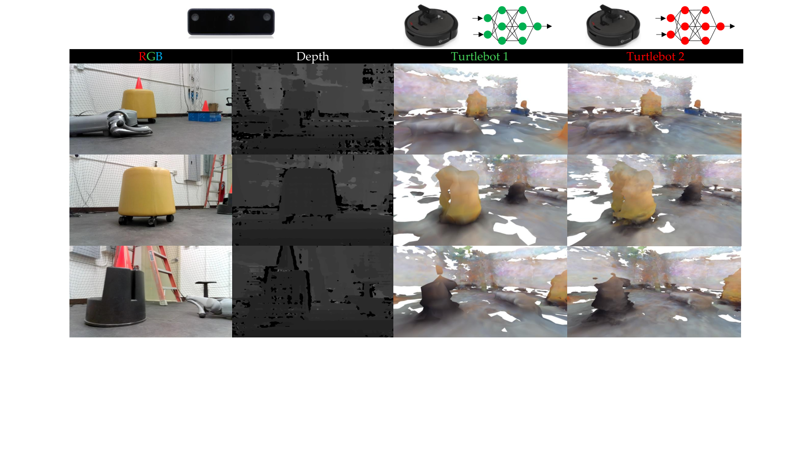
Fig. 8: Comparison of RAMEN reconstructed scene details with corresponding captured images. Each robot only physically visited half of the scene. The complete and similar reconstruction results from both robots indicate successful convergence to consensus. Despite limitations in capturing fine details due to the low quality of depth images, both robots accurately learn the overall scene structure.

V-B Real-World Hardware Experiments

Two manually driven Turtlebots each observe roughly half a scene. Vicon supplies poses, and each robot streams images and poses over WiFi to its own external computer. Mapping runs around one update per second, while the computers exchange neural maps every thirty seconds, reported as a 3.33% communication rate relative to mapping updates. This sparse periodic exchange is different from directly measuring a 3.33% packet-delivery probability.

RAMEN completion scores are 78.47% and 69.66% for the two robots, compared with 63.07% and 39.83% for DiNNO. Artifact distances are 6.50 and 5.87 cm versus 26.43 and 10.76 cm. The reference called ground truth is itself a reconstruction made with one robot and four times as many images, rather than an independent metrology-grade scene mesh. No repeated hardware-trial uncertainty is reported.

The demonstration shows useful map sharing under slow communication and unequal processing speeds. It relies on known poses and human-controlled viewpoints, so it does not establish autonomous exploration, onboard mapping performance, or pose-error robustness.

TABLE II: Hardware experiment results
Robot Method Artifacts (cm) ↓\downarrow Holes (cm) ↓\downarrow Completion Ratio (%) ↑\uparrow
Turtlebot 1 DiNNO 26.43 4.70 63.07
RAMEN 6.50 4.43 78.47
Turtlebot 2 DiNNO 10.76 12.77 39.83
RAMEN 5.87 5.15 69.66

VI Limitations

Counting updates does not distinguish an easy planar region from fine geometry needing many more observations. Keeping and replaying a large keyframe database limits long-duration mapping and can cause storage pressure. Sensor depth noise limits reconstructed detail. Manual robot control introduces selection bias and reproducibility concerns; autonomous active perception is proposed as future work.

VII Conclusion

Reliability-weighted parameter consensus improves the tested neural maps when communication is intermittent, with evidence from dataset replay and a physical two-robot setup. The results support this implementation under the measured conditions, while calibrated uncertainty, broader scaling, pose estimation, and autonomous data collection remain unresolved.

Acknowledgments

The work acknowledges support from three National Science Foundation awards.

Concept demonstration

Open image ↗