At a glance
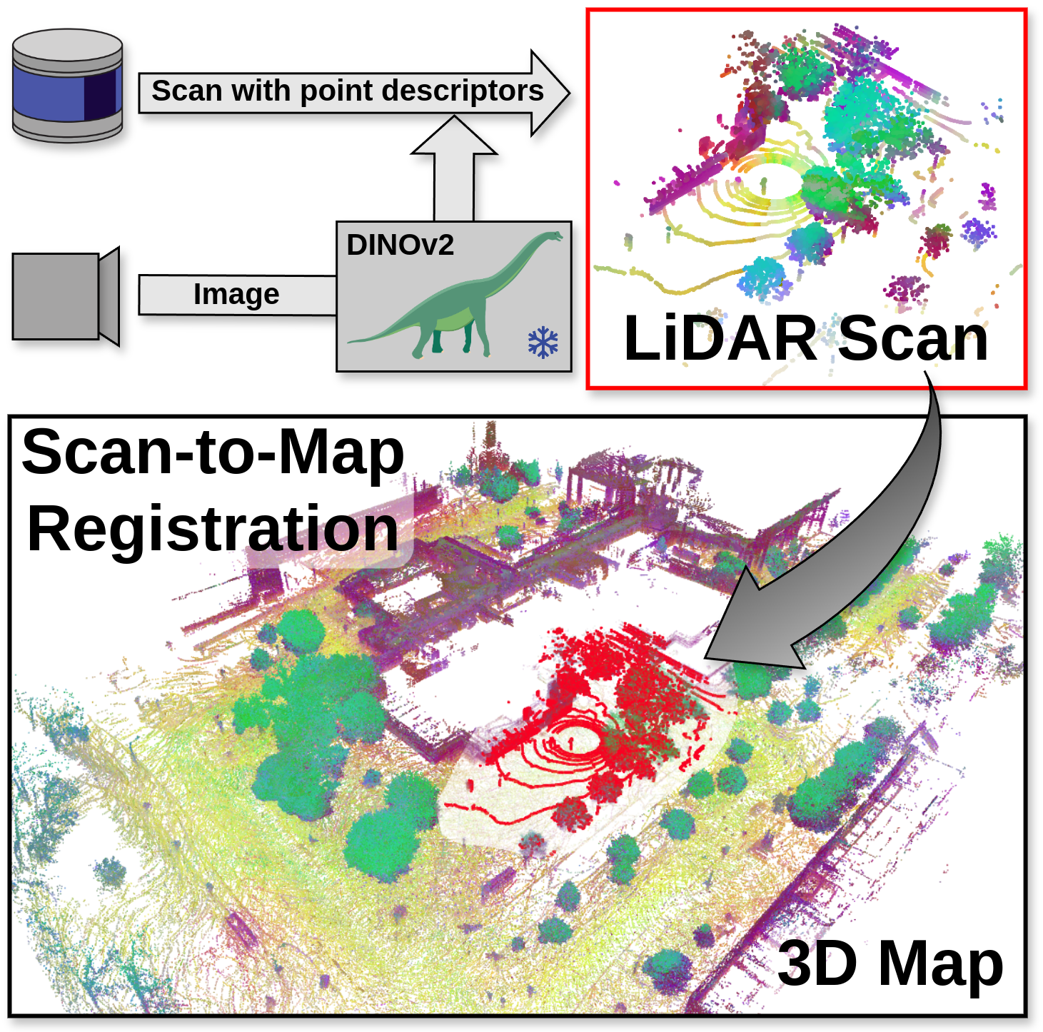
Frozen DINOv2 image features become LiDAR point descriptors through calibrated camera projection. Descriptor matching supplies coarse correspondences for RANSAC, and geometric ICP refines the alignment. On 125 NCLT and 75 Oxford Radar RobotCar scan-to-map pairs, final registration recall reaches 100% and 94.67%, respectively, exceeding the strongest tested LiDAR-only baseline by 24.8 and 17.34 percentage points. The gain uses an additional visual modality and a nearby map region; it does not demonstrate camera-free or unrestricted global localization.
I Introduction
Long-term localization must match a current sparse LiDAR scan to a dense map despite foliage, snow, construction, and changes in point density. Purely geometric descriptors can become ambiguous or fail under domain shifts. This work attaches pretrained DINOv2 features [25] to points, exploiting transferable appearance and implicit semantic information without training a new descriptor on the target dataset. The contribution is a simple multimodal descriptor interface for conventional registration, together with a long-term benchmark. Surround-view images must be available both when mapping and when localizing.
II Related Work
Handcrafted FPFH [29] summarizes local geometry; learned descriptors include patch-based 3DMatch, DIP, and GeDi, and pointwise FCGF, D3Feat, and GCL. Their density and domain sensitivity motivates using visual representations. Earlier semantic approaches reject matches between discrete classes or learn panoptic correspondence, whereas DINOv2 supports continuous feature similarity without assigning explicit classes.
Local ICP and NDT require a useful initial alignment. Global methods instead reject incorrect descriptor matches through RANSAC [16], robust optimization, TEASER, or learned schemes such as PointDSC. This paper changes the descriptors and combines coarse global alignment with geometric ICP. It does not introduce a new rigid-registration solver or establish a formal robustness guarantee.
III Technical Approach
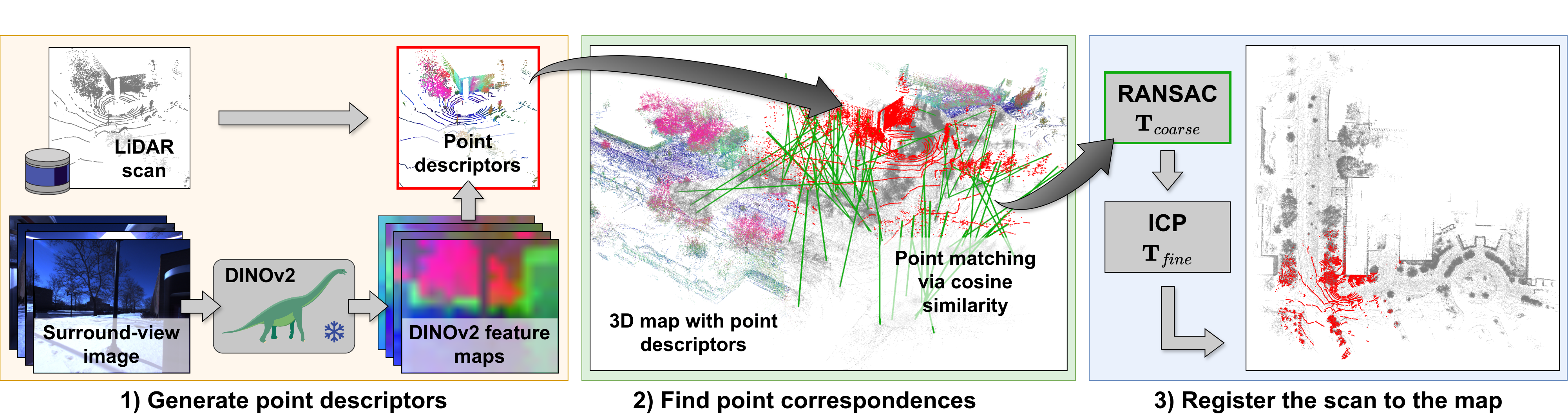
The pipeline extracts image features, associates them with scan/map points, searches for similar descriptors, estimates a coarse rigid transform, and refines it geometrically. Map descriptors are computed offline; current-scan descriptors are computed at test time.
III-A Problem Definition
The inputs are a voxelized 3D map, a current LiDAR scan, and corresponding surround-view RGB observations. The desired output is a six-degree-of-freedom rigid transform in SE(3). A rough position within approximately 100 m selects the relevant map region, potentially using GNSS or place recognition. “Initialization-free” therefore means no accurate initial rigid alignment within that region, rather than no location prior at all. The source’s inequalities relating the subset size k to scan/map sizes m and n are reversed relative to its preceding definitions; they should not be used as a consistent complexity specification.
III-B Point Descriptor Extraction
A frozen DINOv2 encoder converts an image to a dense feature map. The paper gives ViT-S/14 with 384-dimensional features as an example. Known camera–LiDAR calibration projects each 3D point to a pixel, whose feature becomes its descriptor, as retained in Equations 1–3. The same procedure applies to mapping keyframes and incoming scans; voxelization then produces the descriptor-bearing map. Image features transfer across sparse and dense point sets because feature extraction occurs in the image domain.
This association depends on calibration, timing, visibility, and the relationship between camera and LiDAR viewpoints. A point can receive the feature of an occluding foreground object. The paper does not fully specify patch-feature upsampling, multi-view conflict resolution, or descriptor aggregation for multiple observations in a voxel, details that matter for reproduction.
Equations 1–3
| (1) | ||||
| (2) |
| (3) |
III-C Scan-to-Map Registration
The scan is downsampled to roughly one point in eighty before feature matching. For each retained scan point, a similarity search [15] finds the map point with maximum cosine similarity; matches below 0.8 are rejected. Three-point RANSAC estimates the coarse transformation from the surviving pairs. Point-to-point ICP [30] then refines it using the original scan geometry, without DINOv2 descriptors in that final step. The reported performance therefore combines visual correspondence selection with geometric refinement.
Equations 4–5
| (4) | ||||
| (5) |
IV Experiments
Experiments separate easier scan-to-scan matching, long-term scan-to-map registration, and robustness to artificial map changes. They compare descriptors and outlier-rejection schemes under explicit translation/rotation success thresholds.
IV-A Experimental Setup
NCLT [11] contains 27 campus sessions spanning fifteen months, while Oxford Radar RobotCar [6] covers seven recording days over roughly a week and a half. The benchmark uses one mapping session and five registration sessions for NCLT, and one mapping plus three registration sessions for RobotCar. Twenty-five locations per dataset produce 125 and 75 registration pairs. Table I retains the exact dates, times, foliage, snow, and sky conditions; the more-than-one-year separation applies to NCLT, not RobotCar.
Each map accumulates scans at two-meter intervals within 150 m of the sampled position, giving a maximum 300 × 300 m region. KISS-ICP refines mapping poses before 0.25 m voxelization, and dynamic objects are not explicitly removed. Ground-truth transforms are generated by ICP initialized from dataset poses and manually checked. This supplies a practical benchmark, though the reference itself is derived from geometric alignment. The authors state that neither evaluation dataset appears in DINOv2’s LVD-142M training set. These 25 scenes are selected to support all required sessions rather than sampled as an unrestricted deployment distribution.
| Recording date | Map. | Reg. | Time | Sky | Foliage | Snow |
| NCLT | ||||||
| 2012-01-08 | ✓ | Midday | Partly cloudy | – | – | |
| 2012-02-12 | ✓ | Midday | Sunny | – | ✓ | |
| 2012-03-17 | ✓ | Morning | Sunny | – | – | |
| 2012-05-26 | ✓ | Evening | Sunny | ✓ | – | |
| 2012-10-28 | ✓ | Midday | Cloudy | – | – | |
| 2013-04-05 | ✓ | Afternoon | Sunny | – | ✓ | |
| Oxford Radar RobotCar | ||||||
| 2019-01-10 | ✓ | 11:46 | Cloudy | – | – | |
| 2019-01-15 | ✓ | 13:06 | Sunny | – | – | |
| 2019-01-17 | ✓ | 14:03 | Partly cloudy | – | – | |
| 2019-01-18 | ✓ | 15:20 | Cloudy | – | – | |
| Method | NCLT | Oxford Radar RobotCar | |||||||
| Registration | Descriptor | RTE [m] | RRE [] | RR [%] | ICP-RR [%] | RTE [m] | RRE [] | RR [%] | ICP-RR [%] |
| RANSAC | FPFH [29] | 47.5146.54 | 59.9562.21 | 0.00 | 37.60 | 32.5640.18 | 36.8757.25 | 0.00 | 40.00 |
| TEASER++ [31] | FPFH [29] | 60.1534.94 | 121.6748.95 | 0.00 | 0.00 | 69.5141.98 | 129.0149.91 | 0.00 | 0.00 |
| PointDSC [4] | FPFH [29] | 103.1648.70 | 129.7547.90 | 0.00 | 0.00 | 65.2845.19 | 128.0152.22 | 1.33 | 2.67 |
| RANSAC | DIP [27] | 42.9445.26 | 49.8656.08 | 0.00 | 40.00 | 24.5232.96 | 45.0863.06 | 0.00 | 40.00 |
| RANSAC | GeDi [28] | 48.9345.12 | 66.7565.59 | 0.00 | 32.00 | 23.5031.15 | 41.2662.85 | 0.00 | 44.00 |
| RANSAC | FCGF [12] | 22.7433.53 | 31.2048.44 | 0.80 | 64.00 | 20.3432.29 | 37.9262.81 | 1.33 | 49.33 |
| PointDSC [4] | FCGF [12] | 69.5048.40 | 96.8651.55 | 0.00 | 12.00 | 73.5845.43 | 93.5164.32 | 0.00 | 0.00 |
| RANSAC | SpinNet [1] | 33.7042.47 | 41.0055.14 | 0.00 | 54.40 | 23.3935.86 | 30.5756.48 | 0.00 | 56.00 |
| RANSAC | GCL [23] | 15.3526.84 | 23.6745.83 | 13.60 | 75.20 | 11.8125.09 | 21.8448.07 | 30.67 | 77.33 |
| Our method: | |||||||||
| TEASER++ [31] | DINOv2 [25] | 5.2910.02 | 27.9857.09 | 18.40 | 83.20 | 13.4534.93 | 22.1853.69 | 49.33 | 81.33 |
| RANSAC | DINOv2 [25] | 0.400.31 | 1.010.84 | 77.60 | 100.00 | 3.3613.65 | 5.2026.25 | 82.67 | 94.67 |
| RANSAC + ICP | DINOv2 [25] | 0.010.02 | 0.030.06 | 100.00 | 100.00 | 3.1213.63 | 4.5226.21 | 94.67 | 94.67 |
We report the mean and standard deviation of the relative translation error (RTE) and the relative rotation error (RRE) as defined in Sec. IV-B. The registration recall (RR) denotes the success rate, where success is defined as and . The recall after refinement with ICP is listed as ICP-RR. DIP and GeDi are trained on the 3DMatch dataset [32] (RGB-D data). FCGF, SpinNet, GCL, and PointDSC are trained on the KITTI dataset [17] (LiDAR scans).
IV-B Evaluation Metrics
Relative translation error is the Euclidean displacement between estimated and reference translations; relative rotation error is the trace-based angular difference in Equations 6–7. Registration recall counts cases with both translation error below 0.6 m and rotation error below 1.5°. ICP-RR applies that same criterion after refinement. Mean and standard deviation of errors summarize the tested pairs; recall thresholds and the distinction between coarse and refined results are essential to interpreting Table II.
IV-C Scan-to-Map Registration
Baselines include FPFH with RANSAC, TEASER++, or PointDSC; RGB-D-trained DIP/GeDi; and KITTI-trained FCGF, SpinNet, and GCL [23]. RANSAC runs 50,000 iterations without early stopping; baseline matching retains 5,000 correspondences. SpinNet features are limited to 7,500 sampled points by 16 GB GPU memory. The comparison tests existing descriptors under transfer, rather than retraining all methods on the evaluation data or matching the additional visual modality.
Table III examines scan-to-scan registration using 125 KITTI sequence-08 pairs and corresponding NCLT scans, with perturbed reference initialization. KITTI-trained descriptors generally degrade on NCLT. DINOv2 is not evaluated on KITTI because surround-view images are unavailable, and its NCLT errors of 0.56 m/1.44° do not beat the best geometric descriptors in this easier setting. Equation 8 repeats the y translation coordinate with different noise distributions where a third axis would be expected; the original equation is preserved and that ambiguity remains unresolved.
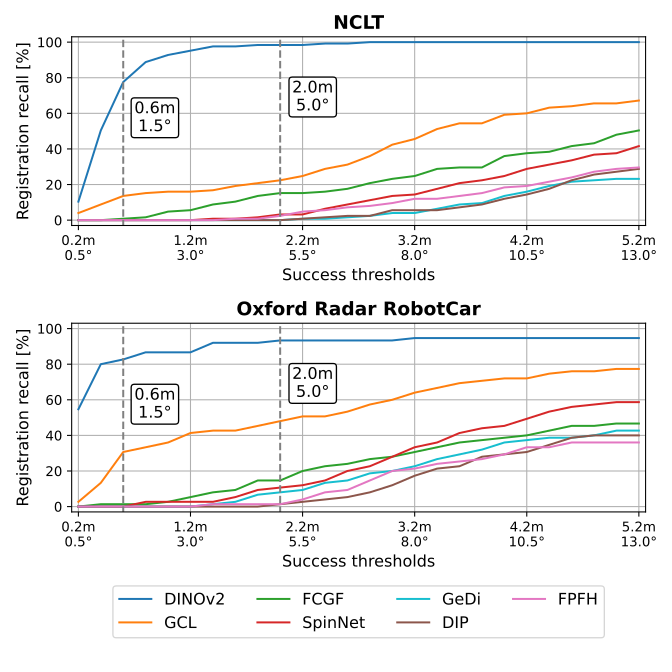
For the main scan-to-map task, DINOv2 plus RANSAC reaches 77.60% coarse recall on NCLT and 82.67% on RobotCar. ICP raises these to 100% and 94.67%, compared with GCL’s 75.20% and 77.33% refined recall. On NCLT, final average error is 0.01 m/0.03°. RobotCar retains a small set of severe failures: its final means are 3.12 m/4.52° with standard deviations 13.63 m/26.21°, so high recall does not imply uniformly tiny errors. DINOv2 plus TEASER++ is weaker, reaching 83.20%/81.33% refined recall.
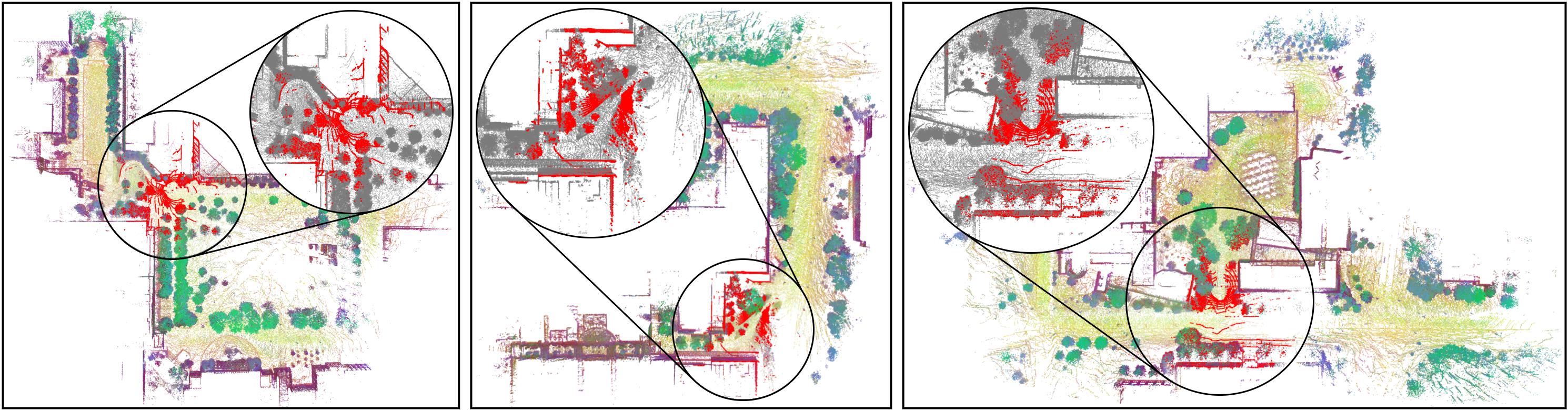
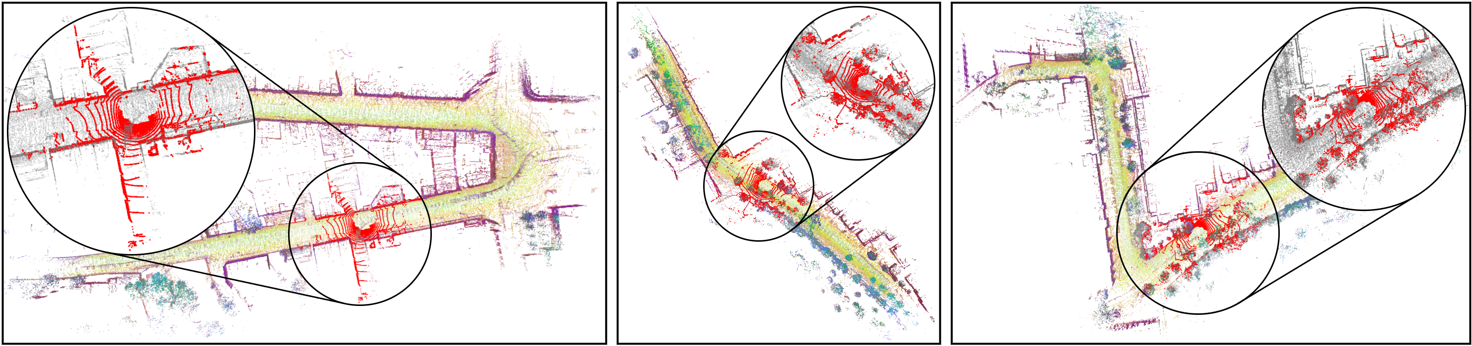
Figure 3 shows that the DINOv2/RANSAC advantage persists across coupled translation/rotation thresholds. The source prose’s broad statement that baselines have zero coarse recall is not universal: GCL has 13.60%/30.67%, and a few others have nonzero values. Figures 6–7 retain three qualitative scenes from each dataset. Colors visualize the first three PCA components of the descriptors, while red indicates the registered scan; these colors are not ground-truth semantic labels.
| Method | KITTI | NCLT | |||
| Registration | Descriptor | RTE [m] | RRE [°] | RTE [m] | RRE [°] |
| Handcrafted descriptor: | |||||
| ICP | n/a | 11.00 | 5.86 | 10.91 | 6.32 |
| RANSAC | FPFH [29] | 0.87 | 1.13 | 1.35 | 3.55 |
| TEASER++ [31] | FPFH [29] | 0.04 | 0.10 | 0.54 | 3.24 |
| PointDSC [4] | FPFH [29] | 0.06 | 0.15 | 2.91 | 9.70 |
| Descriptors trained on 3DMatch [32]: | |||||
| RANSAC | DIP [27] | 0.16 | 0.22 | 0.80 | 2.25 |
| RANSAC | GeDi [28] | 0.50 | 0.73 | 1.71 | 4.25 |
| Descriptors trained on KITTI [17]: | |||||
| RANSAC | FCGF [12] | 0.10 | 0.15 | 0.45 | 1.36 |
| PointDSC [4] | FCGF [12] | 0.07 | 0.14 | 0.51 | 1.64 |
| RANSAC | SpinNet [1] | 0.09 | 0.15 | 0.46 | 1.28 |
| RANSAC | GCL [23] | 0.09 | 0.14 | 0.46 | 1.26 |
| Our method: | |||||
| RANSAC | DINOv2 [25] | – | – | 0.56 | 1.44 |
We underline the effect of a domain change on various point descriptors used as baselines in our experiments. While the descriptors trained on the KITTI dataset [17] perform well within the same domain, they suffer from degradation when tested on the NCLT dataset [11]. Note that PointDSC [4] is also trained on KITTI. Due to the lack of surround-view images, we do not employ our method on KITTI. In contrast to the primary use case of this work, previous studies mostly considered scan-to-scan registration.
Equation 8
| (8) | ||||
IV-D Robustness to Environmental Changes
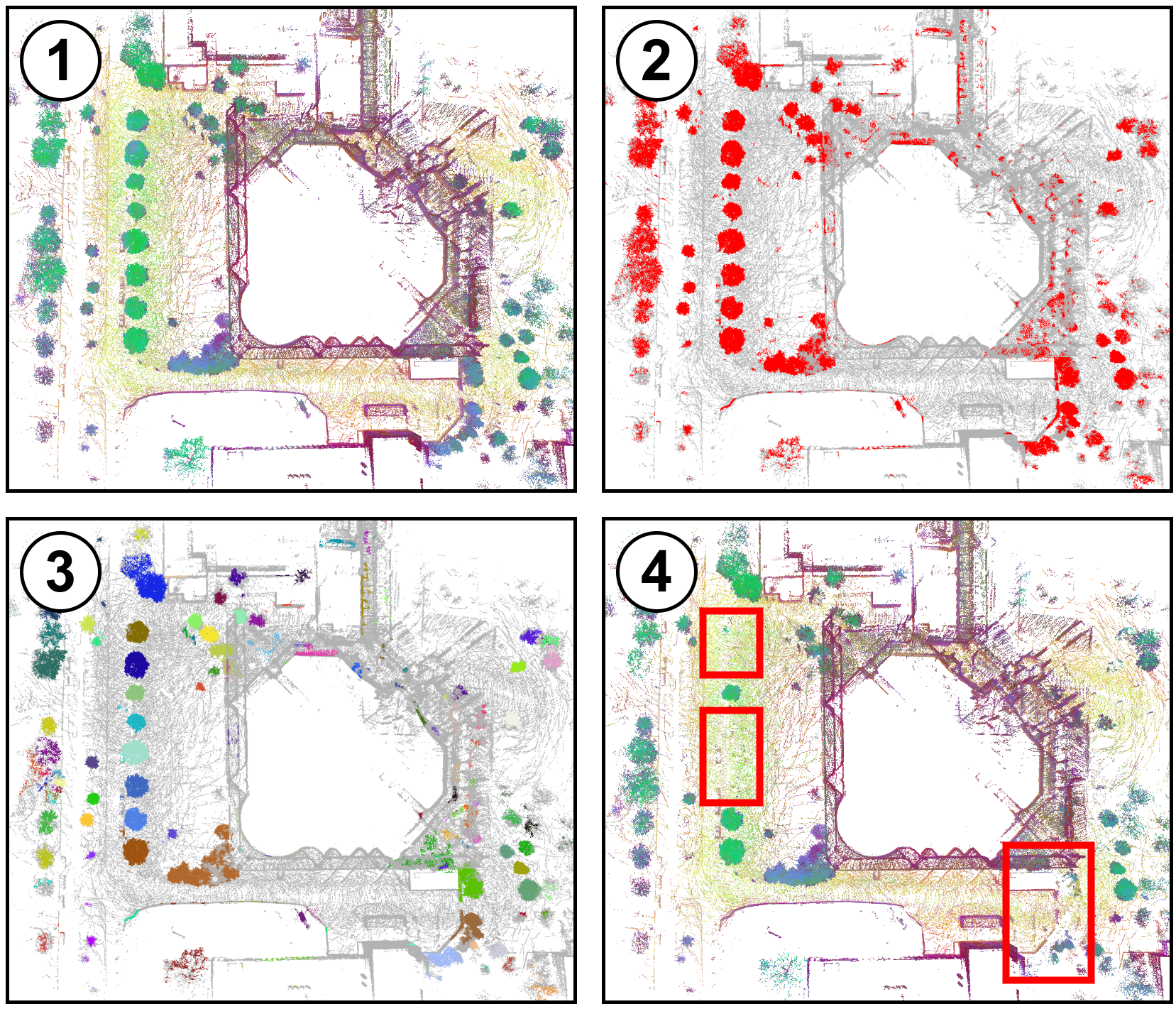
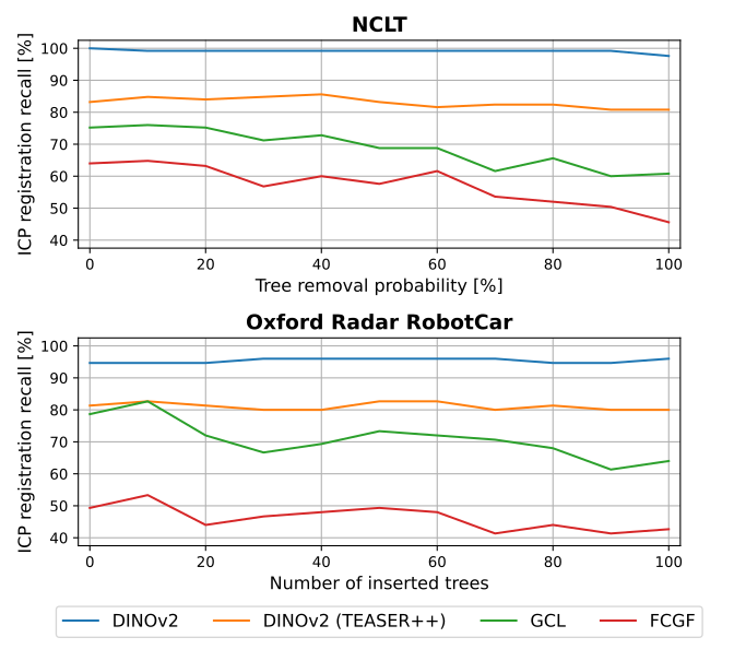
To amplify map mismatch, the authors identify tree-like NCLT points using a human-selected exemplar, a PCA-to-sRGB distance threshold of 50, and HDBSCAN clustering [24]. Each cluster is removed with a chosen probability. In RobotCar, up to 100 extracted NCLT trees are inserted instead. Figures 4–5 preserve the full construction and recall curves. DINOv2 remains comparatively stable while GCL and FCGF degrade; RANSAC is consistently stronger than the DINOv2/TEASER++ variant.
These controlled edits supplement naturally occurring seasonal changes. They test removal/addition of one semantic category, not arbitrary reconstruction, relocation of all landmarks, or severe lighting failure. No repeated-randomization confidence bands are reported, so fine differences between curve points should not be interpreted as established statistical effects.
V Discussion of the Limitations
Camera–LiDAR calibration, time synchronization, ego-motion, occlusion, moving objects, and different fields of view can assign image features to the wrong 3D points. The authors suggest such projection errors explain RobotCar failures, but do not isolate their causal contribution experimentally. Adequate illumination is another dependency. Generalization to very different visual domains is untested. In addition to these stated limits, the paper does not report end-to-end latency, memory use, or ablations separating descriptor quality from camera coverage and feature-extraction choices. Its results support this offline-evaluated multimodal pipeline, not a measured real-time deployment budget.
VI Conclusion
Pretrained image descriptors can make long-term scan-to-map matching substantially more reliable when combined with conventional RANSAC and ICP. The main evidence is the two-dataset recall improvement and resilience to seasonal/tree edits, conditioned on surround-view imagery and a selected map region. Applying visual models to point-cloud projections without cameras and combining visual features with geometric descriptors are proposed future directions, not evaluated capabilities.
Acknowledgment
The authors acknowledge DAAD fellowship support and travel support through the European ELISE and ELSA programs.