Muon is Scalable for LLM Training
Intuition. A matrix update can strongly favor a few directions. In a two-dimensional illustration, its singular values might be 10 and 1: one direction gets ten times the amplification. Muon approximately levels these strengths before choosing the final update scale, rather than merely rescaling individual entries.
Reading the math. Write the momentum matrix as M=UΣVᵀ. U and V describe directions; Σ contains their strengths. The ideal polar update U Vᵀ replaces nonzero strengths by one. Newton–Schulz approximates this with matrix multiplications. It changes the update, not the requirement that the weights themselves be orthogonal; the paper also adds decay and shape-dependent scaling.
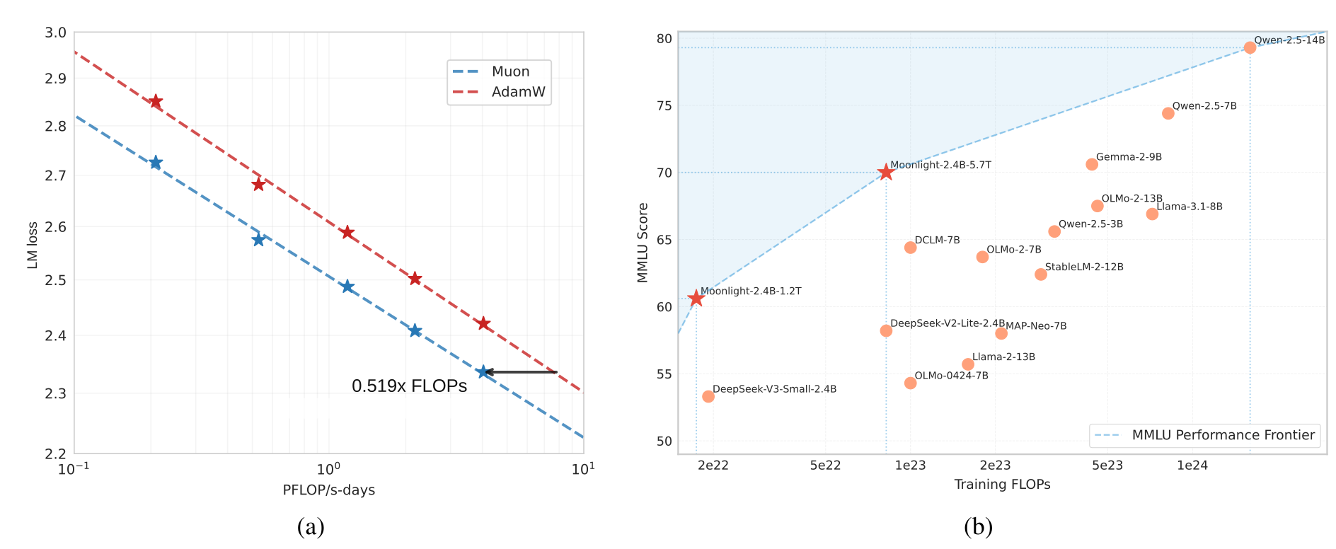
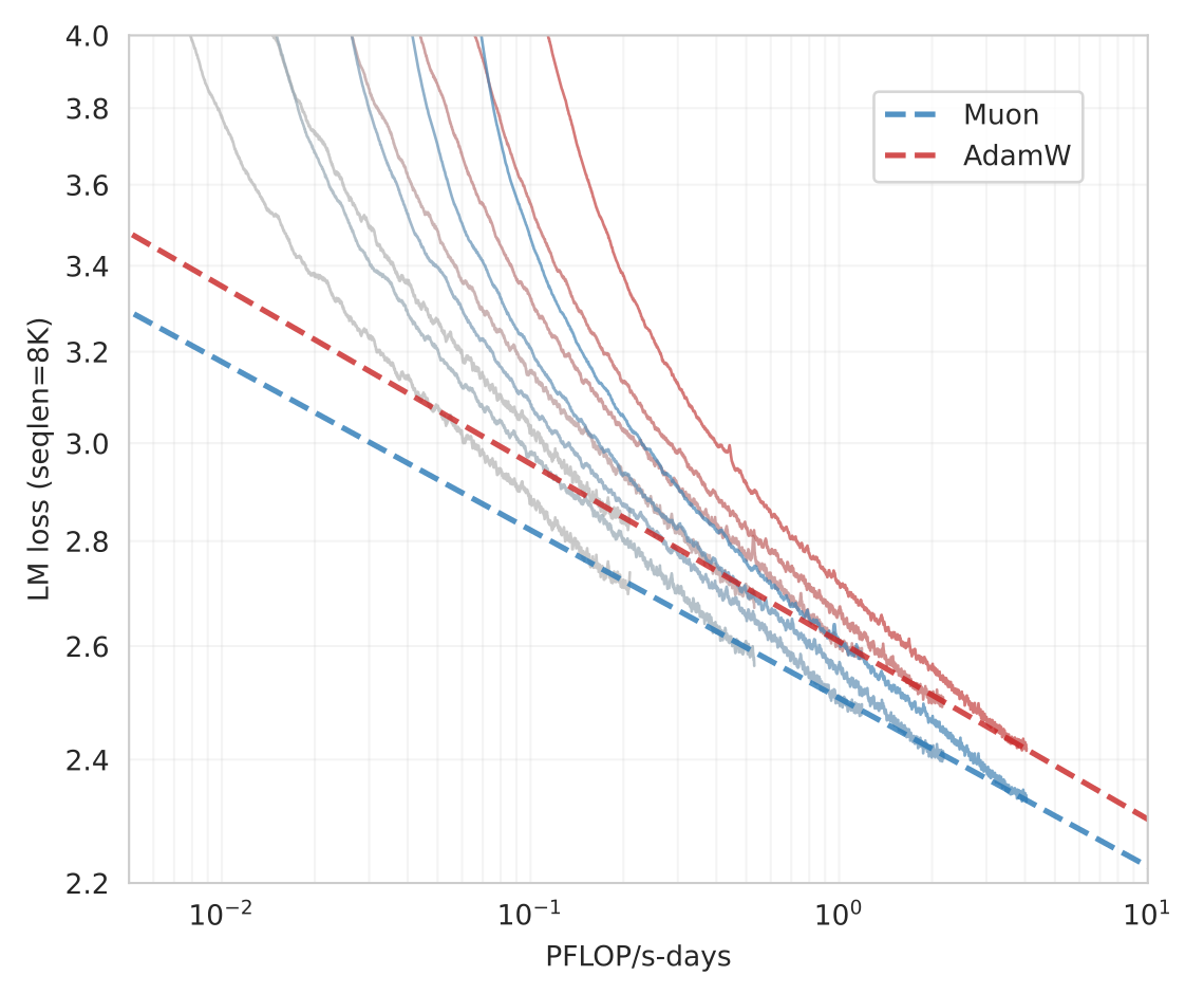
This technical report studies a scalable Muon implementation and releases Moonlight models and checkpoints. Figure 1 summarizes fitted compute/loss curves and comparisons with public models; cross-model frontiers also reflect differences in data and architecture.

At a glance
Adding decoupled weight decay and shape-dependent update scaling makes Muon effective in the authors’ language-model experiments. Compute-optimal fits on dense models suggest approximately half the training FLOPs needed by their AdamW baseline at comparable loss. The resulting Moonlight mixture-of-experts model has about 3 billion active and 16 billion total parameters including embeddings, and is trained on 5.7 trillion tokens. A distributed implementation, pretraining and fine-tuning comparisons, and spectral diagnostics support the case study. The results do not establish a universal twofold saving or superiority for every fine-tuning setting.
1 Introduction
Muon replaces the singular values of gradient momentum approximately, aiming to avoid updates dominated by a few directions. Earlier results were mostly small-scale. This report addresses longer and larger runs, distributed matrix computation, and the interaction between pretraining and supervised fine-tuning. Its key interventions are decay and update-scale matching, followed by a distributed implementation and comparisons against a tuned AdamW baseline. The reported efficiency is an empirical scaling fit over the studied model/data range, while Moonlight demonstrates feasibility at larger scale.
2 Methods
2.1 Background
The Muon Optimizer
Building on Jordan and collaborators [Jordan et al., 2024], Muon accumulates gradient momentum and applies approximate matrix orthogonalization before updating matrix parameters. The implementation uses Nesterov-style momentum, as specified in the footnote. For the ideal polar factor, an SVD M=UΣVᵀ gives U Vᵀ, flattening nonzero singular values. Rectangular and rank-deficient matrices require the corresponding partial-isometry or pseudoinverse interpretation; the inverse-square-root expression alone is not an ordinary inverse in every shape. Finite Newton–Schulz iterations produce an approximation, not exact orthogonality.
Equation 1
| (1) | ||||
Newton-Schulz Iterations for Matrix Orthogonalization
The momentum matrix is first divided by its Frobenius norm, then updated with a quintic matrix polynomial. The coefficients are a=3.4445, b=−4.7750, and c=2.0315, inherited from the original Muon implementation. They favor rapid growth of small singular values; their practical finite-step result should not be confused with an exact polar decomposition or exact convergence of every singular value to one.
Equation 2
| (2) |
Steepest Descent Under Norm Constraints
Following Bernstein and Newhouse [2024], the authors interpret optimizer choice as steepest descent under different norm constraints. Exact polar-factor updates correspond to a spectral-norm constraint; their approximate iteration is discussed in relation to Schatten norms. The argument that an operator norm suits Euclidean hidden representations is a modeling motivation. It does not prove that this geometry always improves generalization over Adam’s adaptive coordinate scaling.
2.2 Scaling Up Muon
Weight Decay
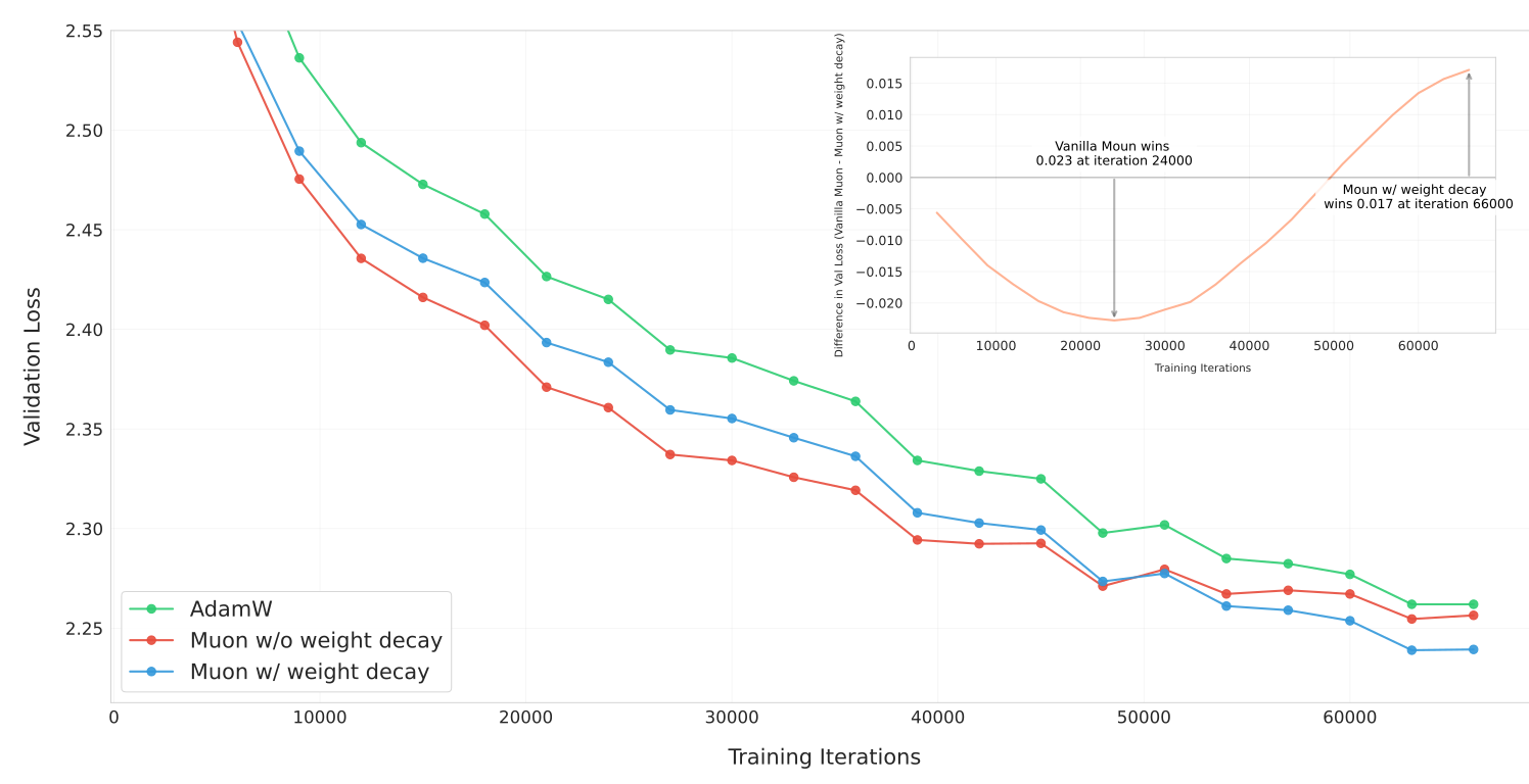
Longer runs without decay show growing weight and output RMS. The proposed update adds AdamW-style decoupled shrinkage, ηλW, outside the orthogonalized momentum. An 800-million-parameter model trained on 100 billion tokens, about five times the compute-optimal token budget used here, initially favors vanilla Muon but later favors Muon with decay. Large magnitudes are discussed as a low-precision training concern; the curves establish the observed benefit in this setup rather than isolating a universal numerical-failure mechanism.
Equation 3
| (3) |
Consistent update RMS
For an exact full-rank polar update of shape A×B, the entrywise RMS is 1/√max(A,B). Without compensation, differently shaped matrices receive different update scales. Multiplication by √max(A,B) cancels this dependence. The result assumes the ideal factor and full rank; finite iterations and rank deficiency can change its exact value. This matters for large feed-forward matrices and small separately parameterized attention heads.
Matching update RMS of AdamW
Some parameters, including normalization scales, embeddings, and the language-model head, continue to use AdamW even when the model is described as Muon-trained. The authors empirically observe AdamW update RMS around 0.2–0.4 and scale Muon’s ideal update by 0.2√max(A,B). This permits reuse of their AdamW learning rate and decay settings. The factor is an empirical calibration, not an optimizer-independent theoretical constant.
Equation 4
| (4) |
Other Hyper-parameters
Five Newton–Schulz steps are used because ten give more accurate orthogonalization without improving the tested performance. Momentum is fixed at 0.95 after no consistent benefit from tuning. These choices favor efficiency in the reported experiments.
2.3 Distributed Muon
ZeRO-1 and Megatron-LM
ZeRO-1 partitions optimizer states across data-parallel workers. Megatron-LM combines this with tensor, pipeline, and expert parallelism, so synchronization can often remain within the relevant data-parallel group.
Method
Elementwise AdamW can operate on a local shard, whereas Muon needs a complete matrix for its polynomial update. Distributed Muon reduce-scatters gradients, applies local momentum, gathers the matrix, computes the full update, keeps the local portion, and all-gathers the updated parameters. The blue lines in Algorithm 1 identify the added operations. Some full-matrix work is consequently repeated while optimizer state remains sharded.
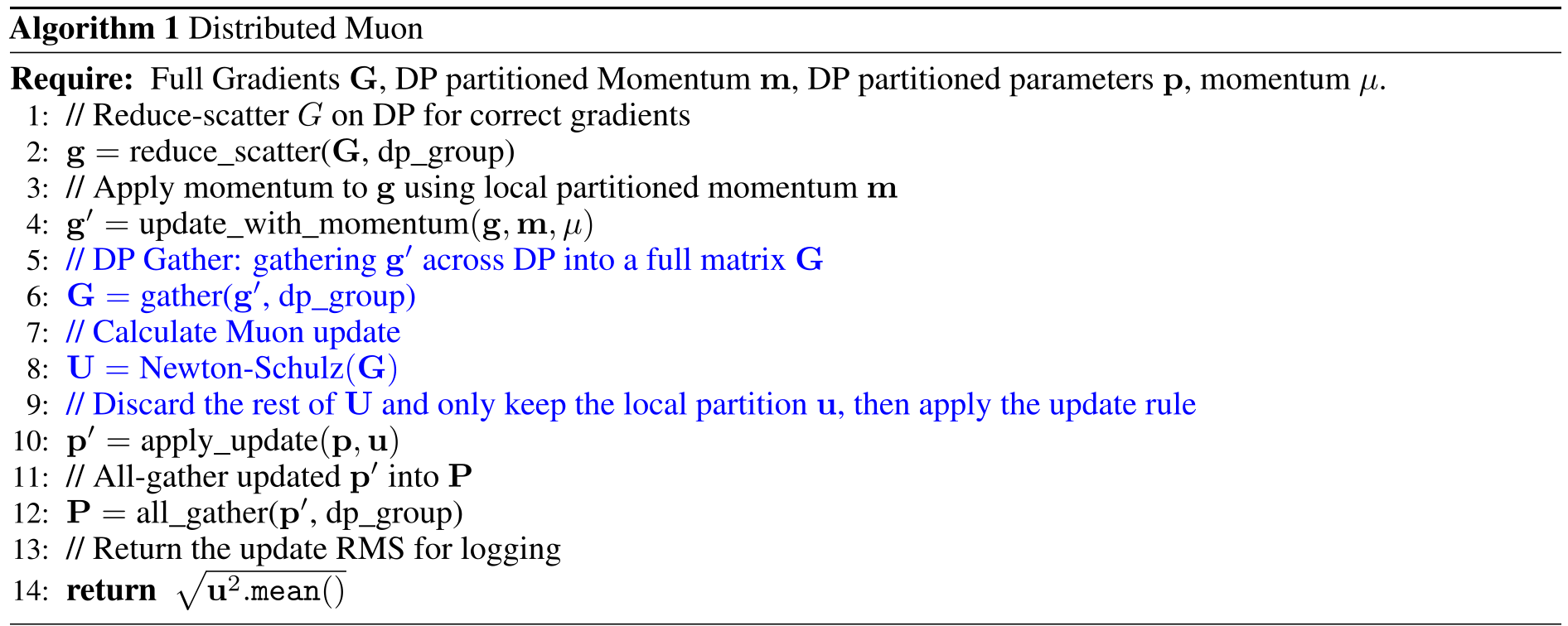
Accessible original algorithm or code markup
Analysis
Muon uses one momentum buffer rather than AdamW’s two, halving this component of optimizer-state memory rather than total training memory. Under the stated communication accounting, workload is between one and 1.25 times the AdamW version, using bfloat16 for the extra gather; tensor parallelism adds another gather. Optimizer work is reported to occupy roughly 1–3% of step time, with no noticeable overall overhead on the authors’ cluster. These latency and communication results depend on sharding, precision, overlap, and hardware.
3 Experiments
3.1 Consistent Update RMS
Three scaling strategies are compared: one global hidden-size factor, exact normalization of each update to RMS 0.2, and a cheaper shape-based learning-rate adjustment. Equations 5–7 retain their square-root factors and the same separate decay term.
Equations 5–7
| (5) |
| (6) |
| (7) |
Analysis
The diagnostic uses an 800-million-parameter model after 4 billion tokens of a 20-billion-token schedule. Replacing SwiGLU with a standard feed-forward block increases the dimension disparity to H×4H. Exact normalization and shape scaling both reduce validation loss from 2.812 to 2.789. Shape scaling approximately doubles the feed-forward weight RMS while leaving the square query matrix closer to the baseline; exact normalization affects both. The authors choose the shape rule because it is cheaper. This is an early-training ablation with a deliberately modified architecture.
3.2 Scaling Law of Muon
Dense Llama-style models range from 399 million to 1.5 billion non-embedding parameters. The AdamW baseline receives a multistage hyperparameter search, and Muon reuses the resulting settings. The fitted loss curves are 2.506 C⁻⁰·⁰⁵² and 2.608 C⁻⁰·⁰⁵⁴ in the paper’s compute units. The approximately 52% compute figure is derived from these fits over the investigated range; the slightly different exponents mean it is not a scale-independent constant, nor a direct measurement of wall-clock acceleration.
| # Params. w/o Embedding | Head | Layer | Hidden | Tokens | LR | Batch Size* |
|---|---|---|---|---|---|---|
| 399M | 12 | 12 | 1536 | 8.92B | 9.503e-4 | 96 |
| 545M | 14 | 14 | 1792 | 14.04B | 9.143e-4 | 128 |
| 822M | 16 | 16 | 2048 | 20.76B | 8.825e-4 | 160 |
| 1.1B | 18 | 18 | 2304 | 28.54B | 8.561e-4 | 192 |
| 1.5B | 20 | 20 | 2560 | 38.91B | 8.305e-4 | 256 |
*In terms of number of examples in 8K context length.
3.3 Pretraining with Muon
Model Architecture
Moonlight follows a modified DeepSeek-V3-Small architecture with 2.24 billion active and 15.29 billion total parameters excluding embeddings, approximately 3B/16B including them. Appendix C describes the changes, which matter in comparisons to public models.
Pretraining Data
Pretraining uses the authors’ data mixture referenced to their separate data report, with a maximum context length of 8K. The optimizer paper does not itself fully specify that proprietary mixture.
Pretraining
The first 33 billion tokens include a 2,000-step warmup to learning rate 4.2×10⁻⁴. Cosine decay then reaches 4.2×10⁻⁵ at 5.2 trillion tokens; batch size doubles from 2,048 to 4,096 examples after 200 billion tokens. A final 500-billion-token cooldown briefly raises the rate to 10⁻⁴, then decays it linearly to zero on higher-quality math, code, and reasoning data. Decay remains 0.1. The auxiliary-free routing-bias update rate is 10⁻³ in the first two stages and zero in the last.
Evaluation Benchmarks
Evaluation spans English knowledge/reasoning, code generation, mathematics, and Chinese knowledge/reasoning. The tables retain dataset names, shot counts, exact-match or pass@1 metrics, and missing entries; scores from different protocols should not be pooled as one common measure.
Performance
At 1.2 trillion tokens, the strongest optimizer comparison is Moonlight versus Moonlight-A with the same training setup and AdamW. Muon improves most reported tasks, especially code and math, but BBH is lower: 43.2 versus 45.3. These are intermediate checkpoints before cooldown. At 5.7 trillion tokens, Moonlight reaches MMLU 70.0 and HumanEval 48.1 and is competitive with similarly active-sized public models; Qwen2.5-3B remains higher on GSM8K, 79.1 versus 77.4. Public-model comparisons also change data, architecture, token count, and sometimes unknown optimizer settings, so they cannot attribute every difference to Muon. The claimed frontier is with respect to the selected models and reported compute estimates.
| Benchmark (Metric) | DSV3-Small | Moonlight-A@1.2T | Moonlight@1.2T | |
|---|---|---|---|---|
| Activated Params† | 2.24B | 2.24B | 2.24B | |
| Total Params† | 15.29B | 15.29B | 15.29B | |
| Training Tokens | 1.33T | 1.2T | 1.2T | |
| Optimizer | AdamW | AdamW | Muon | |
| English | MMLU | 53.3 | 60.2 | 60.4 |
| MMLU-pro | - | 26.8 | 28.1 | |
| BBH | 41.4 | 45.3 | 43.2 | |
| TriviaQA | - | 57.4 | 58.1 | |
| Code | HumanEval | 26.8 | 29.3 | 37.2 |
| MBPP | 36.8 | 49.2 | 52.9 | |
| Math | GSM8K | 31.4 | 43.8 | 45.0 |
| MATH | 10.7 | 16.1 | 19.8 | |
| CMath | - | 57.8 | 60.2 | |
| Chinese | C-Eval | - | 57.2 | 59.9 |
| CMMLU | - | 58.2 | 58.8 |
† The reported parameter counts exclude the embedding parameters.
| Benchmark (Metric) | Llama3.2-3B | Qwen2.5-3B | DSV2-Lite | Moonlight | |
|---|---|---|---|---|---|
| Activated Param† | 2.81B | 2.77B | 2.24B | 2.24B | |
| Total Params† | 2.81B | 2.77B | 15.29B | 15.29B | |
| Training Tokens | 9T | 18T | 5.7T | 5.7T | |
| Optimizer | AdamW | Unknown | AdamW | Muon | |
| English | MMLU | 54.7 | 65.6 | 58.3 | 70.0 |
| MMLU-pro | 25.0 | 34.6 | 25.5 | 42.4 | |
| BBH | 46.8 | 56.3 | 44.1 | 65.2 | |
| TriviaQA‡ | 59.6 | 51.1 | 65.1 | 66.3 | |
| Code | HumanEval | 28.0 | 42.1 | 29.9 | 48.1 |
| MBPP | 48.7 | 57.1 | 43.2 | 63.8 | |
| Math | GSM8K | 34.0 | 79.1 | 41.1 | 77.4 |
| MATH | 8.5 | 42.6 | 17.1 | 45.3 | |
| CMath | - | 80.0 | 58.4 | 81.1 | |
| Chinese | C-Eval | - | 75.0 | 60.3 | 77.2 |
| CMMLU | - | 75.0 | 64.3 | 78.2 |
† The reported parameter counts exclude the embedding parameters.‡ We tested all listed models with the full set of TriviaQA.
3.4 Dynamics of Singular Spectrum
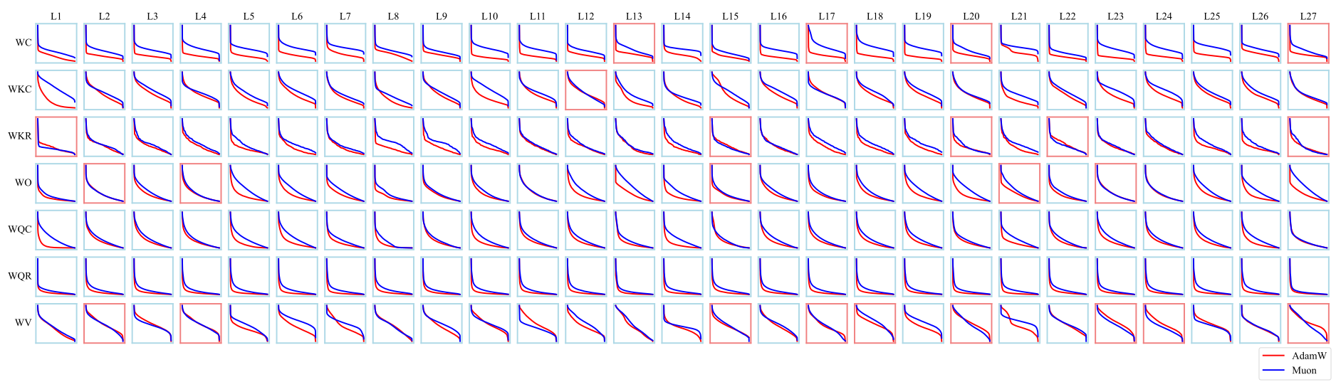
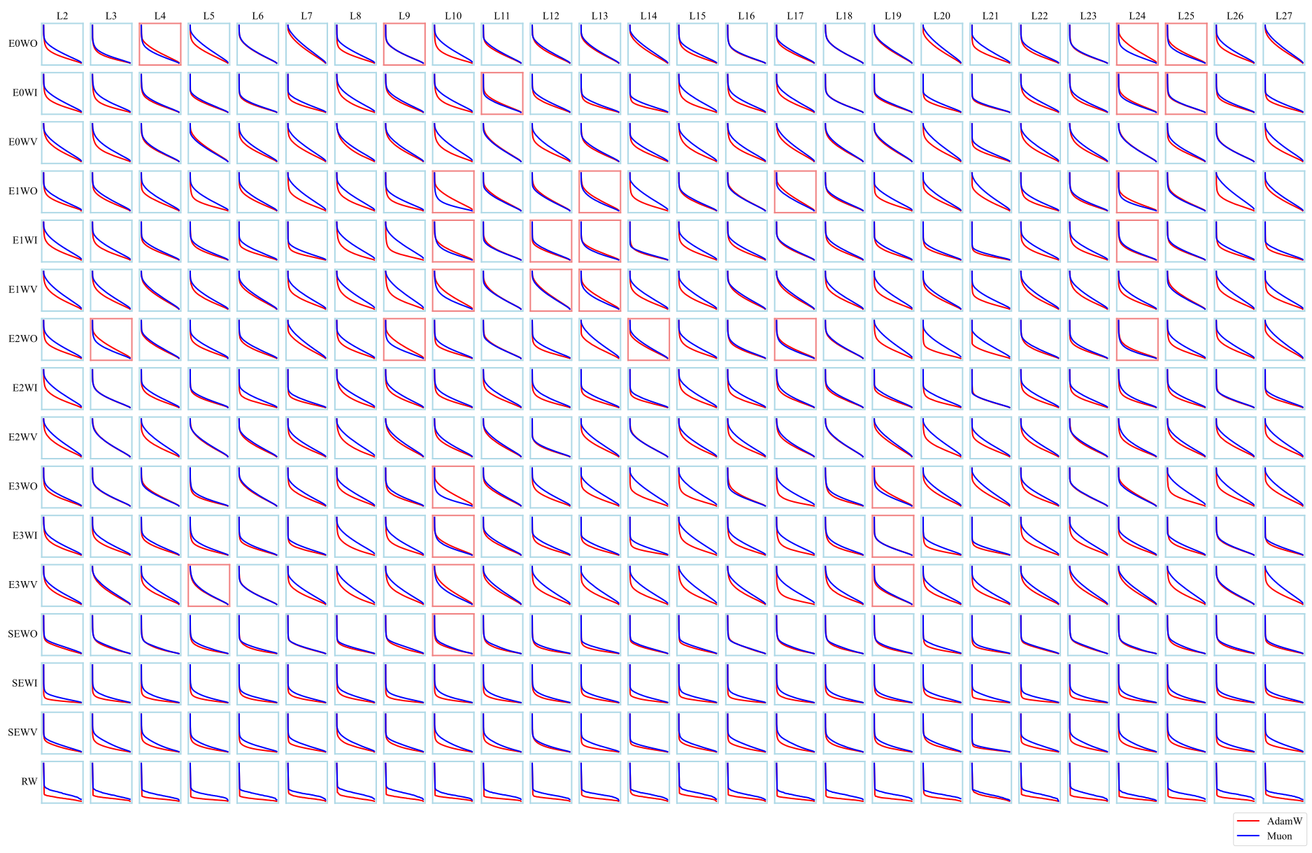
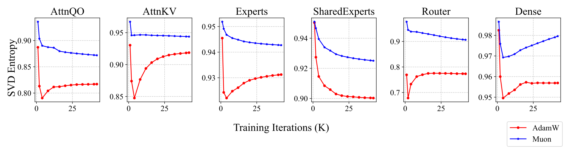
Normalized entropy of squared singular values measures how evenly a weight matrix distributes its spectral energy. Muon-trained weights have higher group-average entropy across the plotted checkpoints, especially router matrices, and more than 90% of inspected matrices have higher entropy at 1.2 trillion tokens. Only a small subset of experts is analyzed. These are weight-spectrum observations; they are consistent with the proposed explanation but do not directly measure all update directions or prove that increased entropy causes better task performance.
Equation
3.5 Supervised Finetuning (SFT) with Muon
The best tested combination uses Muon for both pretraining and supervised fine-tuning. Switching optimizers gives mixed results, and applying Muon only during fine-tuning does not show a general advantage.
3.5.1 Ablation Studies on the Interchangeability of Pretrain and SFT Optimizers
The 1.2-trillion-token Moonlight and Moonlight-A checkpoints are fine-tuned for two epochs on Tulu-3 SFT data at 4K context, with a linearly decaying learning rate starting at 5×10⁻⁵. The Muon/Muon combination is best on all four reported metrics. The complete four-way table is retained, so improvements from the pretrained checkpoint can be distinguished from the fine-tuning optimizer choice.
| Benchmark (Metric) | # Shots | Moonlight-1.2T | |||
|---|---|---|---|---|---|
| Pretraining Optimizer | - | Muon | AdamW | Muon | AdamW |
| SFT Optimzier | - | Muon | Muon | AdamW | AdamW |
| MMLU (EM) | 0-shot (CoT) | 55.7 | 55.3 | 50.2 | 52.0 |
| HumanEval (Pass@1) | 0-shot | 57.3 | 53.7 | 52.4 | 53.1 |
| MBPP (Pass@1) | 0-shot | 55.6 | 55.5 | 55.2 | 55.2 |
| GSM8K (EM) | 5-shot | 68.0 | 62.1 | 64.9 | 64.6 |
3.5.2 SFT with Muon on public pretrained models
Qwen2.5-7B is fine-tuned on packed 8K Tulu-3 data with cosine decay from 2×10⁻⁵ to 2×10⁻⁶. The report calls the results comparable, but Muon is numerically below Adam on all four listed metrics, including GSM8K 85.8 versus 89.8. This ablation supports caution about simply switching an existing pretrained model to Muon.
| Benchmark (Metric) | # Shots | Adam-SFT | Muon-SFT |
|---|---|---|---|
| Pretrained Model | - | Qwen2.5-7B | |
| MMLU (EM) | 0-shot (CoT) | 71.4 | 70.8 |
| HumanEval (Pass@1) | 0-shot | 79.3 | 77.4 |
| MBPP (Pass@1) | 0-shot | 71.9 | 71.6 |
| GSM8K (EM) | 5-shot | 89.8 | 85.8 |
4 Discussions
The discussion identifies three unresolved extensions.
Incorporating All Parameters into the Muon Framework
The current system is hybrid: some parameters still use AdamW. A method that applies the same Muon framework to every parameter is left for future research.
Extending Muon to Schatten Norms
General Schatten-norm geometries are proposed as a possible extension beyond the spectral-norm interpretation. Their benefits are not established in this report.
Understanding and Solving the Pretraining-Finetuning Mismatch
The reason for the pretraining/fine-tuning optimizer mismatch remains unresolved. Understanding it is important before reusing the large pool of AdamW-pretrained checkpoints with a different fine-tuning optimizer.
5 Conclusions
The report demonstrates a practical large-scale Muon-based training recipe, not a theorem that it should replace AdamW everywhere. Decay, matrix-shape scaling, distributed implementation, and a hybrid treatment of parameters collectively produce strong results in the studied setup. Data and architecture differences, fitted scaling extrapolations, and the fine-tuning mismatch limit broader conclusions.
Appendix A Update RMS
Proof of Lemma 1
For a rank-r partial isometry of size n×m, orthonormality gives squared Frobenius norm r and entrywise RMS √(r/(mn)). For full rank with n≥m, this becomes 1/√n. The proof explains the shape correction and why rank deficiency changes the exact scale. The displayed sums are retained; cancellation of cross terms is understood after summing over orthogonal rows or columns.
Equations
Consistent Update RMS Across Muon and AdamW
A small-model ablation compares target update RMS values 0.05, 0.1, 0.2, 0.4, and 0.8 after about 2 billion tokens. Values 0.2 and 0.4 perform similarly and better than the other tested values; 0.2 is selected. This short-run calibration supports that recipe but does not establish a universal optimum.
| Optimizer | AdamW | 0.05 RMS* | 0.1 RMS | 0.2 RMS | 0.4 RMS | 0.8 RMS |
|---|---|---|---|---|---|---|
| LM training loss | 3.512 | 3.355 | 3.239 | 3.198 | 3.199 | 3.386 |
| LM validation loss | 3.679 | 3.503 | 3.374 | 3.325 | 3.314 | 3.543 |
| AttnQ weight RMS | 1.01e-2 | 5.74e-3 | 8.44e-3 | 1.57e-2 | 2.95e-2 | 7.23e-2 |
| Mlp weight RMS | 1.25e-2 | 8.01e-3 | 1.27e-2 | 2.35e-2 | 4.51e-2 | 8.73e-2 |
*Except the first column, all other candidates are using Muon with controlled RMS.
Appendix B AdamW Baseline Scaling Law
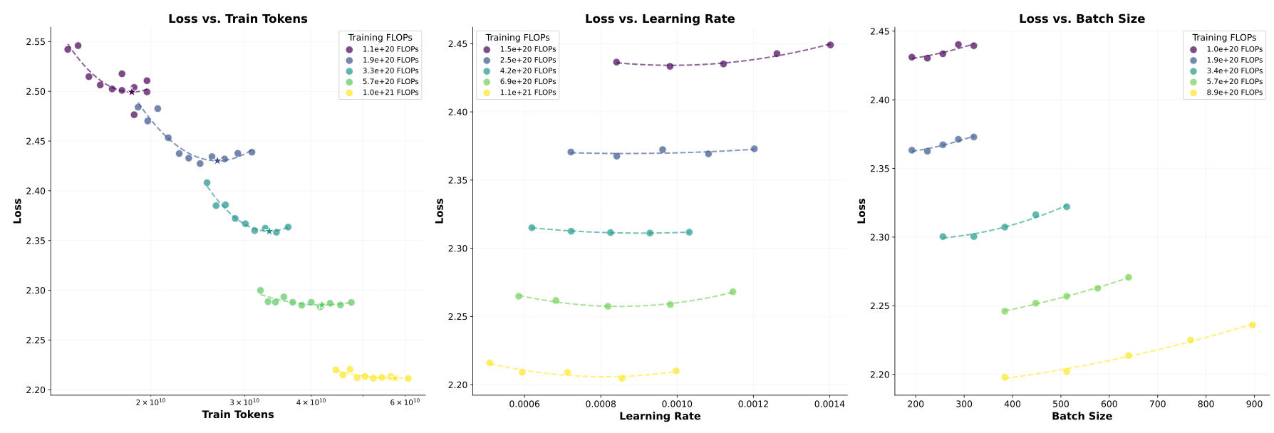
On the authors’ dataset, fitted compute-optimal model and token counts scale approximately as C⁰·⁵¹¹ and C⁰·⁴⁸⁹. The appendix also reports empirical learning-rate and batch-size formulas. Their coefficients depend on the compute and parameter conventions used in these experiments.
Hyper-Parameters Search
For each budget, model size and token count are varied under the approximation C=6ND. Learning rate and batch size are then refined with grid searches; this process is repeated two or three times with narrower ranges. The observed loss bowls motivate the fitted choices, but a finite grid does not certify a global optimum over every training recipe.
Appendix C Model Architecture
Moonlight starts from a DeepSeek-V3-Small-like mixture-of-experts architecture and makes the following specific changes.
Multi-token Prediction (MTP)
Multi-token-prediction layers are omitted because they did not give a significant pretraining benefit in the authors’ experiments.
Auxfree Bias Update
The expert-bias update subtracts the mean sign of expert load deviations from each signed increment. This controls the common bias drift while leaving top-k ranking unchanged for a common additive shift. The complete source update remains visible.
Gate Scaling Factor
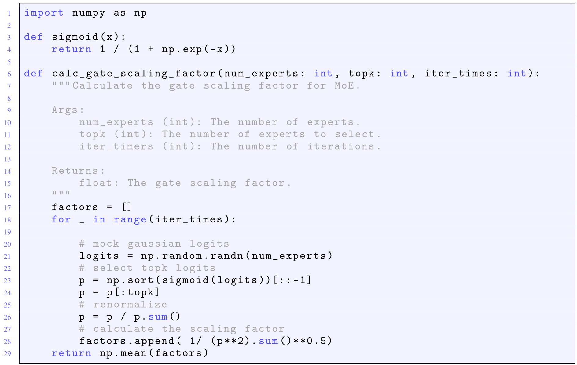
A routing-output scale of 2.446 is selected to approximately match dense-block output RMS. Figure 6 retains the exact Python code: sample Gaussian logits, apply sigmoid, choose and renormalize top-k weights, then average the inverse square root of their squared sum. This is a calibration under that synthetic-logit model.
Accessible original algorithm or code markup
Appendix D Training Stability
Figure 7 preserves all four training-dynamics panels, including attention-logit diagnostics that qualify the smooth-loss observation.

No Loss or Grad Norm Spike
The authors report no loss or gradient-norm spikes in the Moonlight run. This describes the observed traces rather than a stability guarantee across seeds and settings.
Max Attention Logit
Some layers’ maximum attention logits exceed 100 early in training, while AdamW controls this statistic better. The fraction above 100 remains small, around 10⁻⁴, and maximum values later decline. Stable loss and gradient norm therefore coexist with an extreme-logit concern; the separate panels should not be collapsed into an unqualified stability claim.
RMSNorm Gamma Weight Decay
Applying decay to the RMSNorm gamma parameter is reported crucial for preventing excessive layer-output RMS in this recipe.
Appendix E Comparison with More Expensive Models
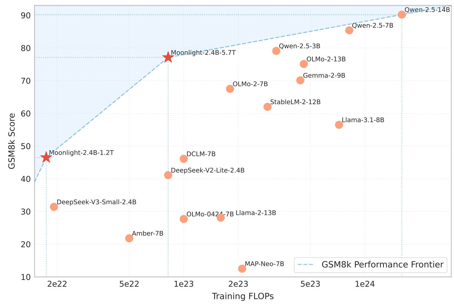
Moonlight is also compared with models trained using more compute, including Llama3.1-8B, Gemma2-9B, and Qwen2.5-7B. It beats some scores and trails others; for example Qwen2.5-7B is higher on MMLU, HumanEval, MBPP, GSM8K, and MATH. Figure 8 places selected GSM8K scores against reported FLOPs. These comparisons contextualize efficiency without isolating optimizer causality.
| Benchmark (Metric) | Moonlight | LLAMA3.1-8B | Gemma2-9B | Qwen2.5-7B | |
|---|---|---|---|---|---|
| Larger Training Compute Model | |||||
| Activated Param† | 2.24B | 7.38B | 8.32B | 6.83B | |
| Total Params† | 15.29B | 7.38B | 8.32B | 6.83B | |
| Training Tokens | 5.7T | 15T | 8T | 18T | |
| Optimizer | Muon | AdamW | Unknown | Unknown | |
| English | MMLU | 70.0 | 66.7 | 71.3 | 74.2 |
| MMLU-pro | 42.4 | 37.1 | 44.7 | 45.0 | |
| BBH | 65.2 | 57.7 | 68.2 | 70.4 | |
| TriviaQA‡ | 66.3 | 70.3 | - | 60.0 | |
| Code | HumanEval | 48.1 | 37.2 | 37.8 | 57.9 |
| MBPP | 63.8 | 47.6 | 62.2 | 74.9 | |
| Math | GSM8K | 77.4 | 57.2 | 70.7 | 85.4 |
| MATH | 45.3 | 20.3 | 37.7 | 49.8 | |
† The reported parameter counts exclude the embedding parameters.‡ We test all listed models with the full set of TriviaQA.
Appendix F Singular Value Distributions of Weight Matrices
The appendix preserves the complete attention and feed-forward spectral grids, normalizing each spectrum by its largest singular value and marking lower-entropy Muon cases with red spines. Projection labels distinguish compressed key/value representations, RoPE components, experts, shared experts, and router matrices. Most curves are flatter with Muon. The Figure 10 caption names three selected experts, whereas the displayed grid also includes an E1 group alongside E0, E2, and E3; both are retained as printed. The sampled matrices and descriptive entropy statistic do not establish a universal performance mechanism.