Literature
Display
← All papers

DDAT: Diffusion Policies Enforcing Dynamically Admissible Robot Trajectories

Jean-Baptiste Bouvier · Kanghyun Ryu · Qiayuan Liao · Koushil Sreenath · Negar Mehr

· Robotics: Science and Systems 2025 ↗

Robotics12 min text · CondensedOriginal paper ↗
Contents

Overview

This edition follows the eighteen-page April 2025 arXiv v2 paper. It retains the full method, experiments, limitations, and implementation appendices. The PDF skips Figure 2, while the HTML numbers the same nine figures consecutively; content matching, rather than label equality alone, verifies retention. Several displayed equation numbers also differ between the two versions.
Original compound figure with every panel and label in the source arrangement.
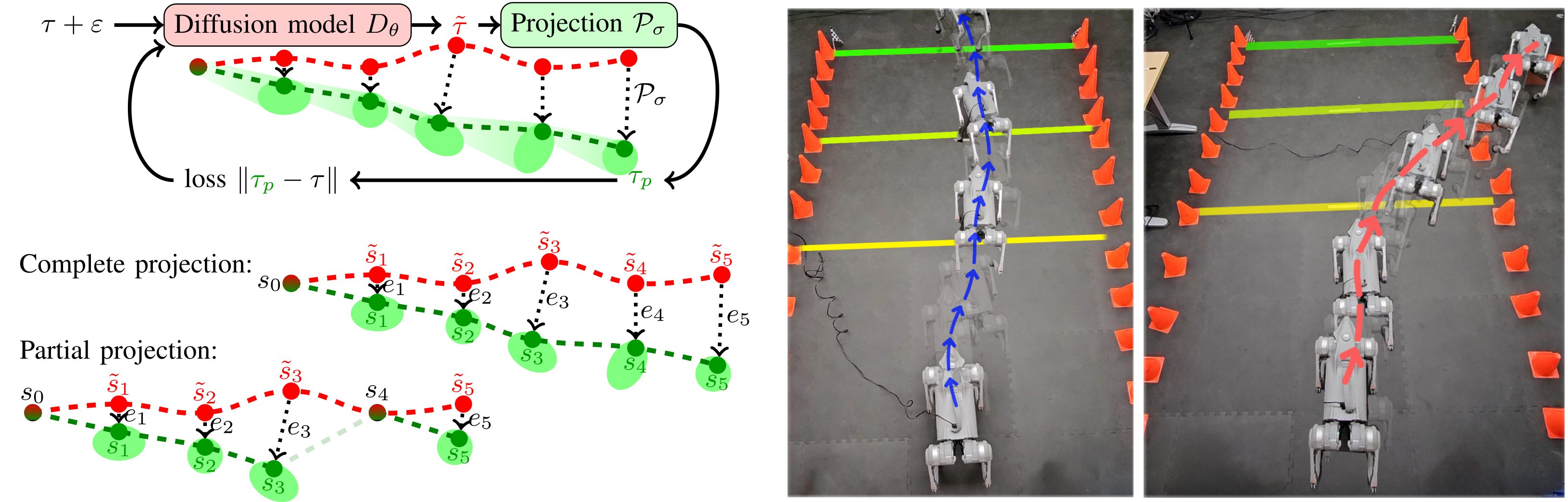
Fig. 1: (top left) Overview of Diffusion policies for Dynamically Admissible Trajectories (DDAT). Diffusion model DθD_{\theta} is trained to predict a trajectory τ~\tilde{\tau} given a trajectory τ\tau from the training dataset corrupted by noise ε\varepsilon. If the noise level σ\sigma of signal ε\varepsilon is sufficiently small, 𝒫σ\mathcal{P}_{\sigma} projects τ~\tilde{\tau} to the dynamically admissible trajectory τp\tau_{p}. The loss ‖τp−τ‖\|{\color[rgb]{0,0.5,0}\tau_{p}}-\tau\| is used to update DθD_{\theta}. (bottom left) To smoothly incorporate projections into the training and inference of our diffusion models we use partial projections of infeasible trajectories. The total projection error ∑et\sum e_{t} is significantly reduced by not projecting s~4\tilde{s}_{4} on the reachable set of s3s_{3}. (right) Demonstration of DDAT on the Unitree GO2. A vanilla diffusion policy fails at walking through the cones in open-loop. By accounting for the quadruped’s dynamics our open-loop diffusion policy succeeds in following the corridor.

At a glance

DDAT combines trajectory diffusion with chronological dynamics projections. A deterministic simulator supplies successor states even when its equations are unavailable. Convex reachable-set approximations improve state plans but can fail with contact-induced nonconvexity; directly rolling out predicted or corrected actions enforces simulator dynamics. Experiments include six simulated robots and open-loop quadruped hardware trials. Projection timing matters, while adding projections during training does not improve the reported results.

I Introduction

Denoised state sequences need not obey a robot’s dynamics, especially under limited actuation. Replanning can compensate but costs computation. DDAT instead inserts chronological corrections into generation, with variants that trade state-plan fidelity, exact simulator rollout, and cost. Its aim is longer open-loop plans; feasibility under a model does not guarantee task success, collision avoidance, or accurate physical execution.

II Related Works

The related work separates constraint enforcement from the choice to diffuse states, actions, or both. These choices offer different guarantees and computational costs. The comparison concerns the reviewed literature and does not imply that every form of diffusion planning lacks a dynamics-aware component.

II-A Enforcing constraints on diffusion models

Soft guidance encourages a property through scores or losses; hard projection attempts to enforce a specified constraint on each sample. Dynamical consistency is harder than an independent per-state bound because every corrected state changes the reachable set of its successor.

II-A 1 Soft constraints

Classifier guidance, classifier-free guidance, and additional loss terms can steer samples toward constraints without ensuring every sample satisfies them. Sampling and selecting many candidates can improve observed quality but does not convert such encouragement into an exact guarantee.

II-A 2 Hard constraints

Hard constraints have been enforced by clipping, reflection, manifold constructions, and projection. Interleaving correction with denoising can improve quality over a final correction alone, yet projection at high noise can distort samples. The paper extends these ideas to chronological robot dynamics, with guarantees depending on the particular projector.

II-B Diffusion planning

Diffusing actions, states, or joint state–action sequences changes where dynamical consistency comes from. The comparison distinguishes a generated plan from the physical trajectory obtained when its controls are executed.

II-B 1 Dynamic feasibility enforced by planning on actions

An admissible action sequence produces a dynamics-consistent simulator rollout by construction, as in action-based approaches such as Diffusion Policy. Predicting volatile action sequences may be harder than predicting smooth state sequences, although this is an empirical tendency rather than a universal limitation. Additional temporal or inverse models offer alternative tradeoffs.

II-B 2 Diffusion planning on states

State diffusion directly represents desired motion but supplies no automatic transition feasibility. Replanning, infeasibility guidance, constraint optimization, and control-barrier methods address parts of this problem. DDAT targets nonlinear black-box dynamics, while noting that some earlier dynamics-constrained studies evaluated linear systems.

II-B 3 Diffusion planning on states and actions

Joint state–action prediction, exemplified by Diffuser, can learn temporal coherence without enforcing the simulator equations. Learned inverse dynamics can also introduce error. Using diffusion to initialize a separate trajectory optimizer is another route; DDAT instead compares corrections integrated into the diffusion process.

III Framework

The assumed system is deterministic and discrete time, with known admissible action bounds and a simulator that returns the next state for any queried state–action pair. Black-box means unavailable equations, not unavailable dynamics queries. A dataset of representative admissible trajectories supplies the imitation target.

Equation 1
st+1=f⁡(st,at),at∈𝒜,s0∼𝒰⁡(𝒮0),s_{t+1}=f\big(s_{t},a_{t}\big),\quad a_{t}\in\mathcal{A},\quad s_{0}\sim\mathcal{U}(\mathcal{S}_{0}), (1)

III-A Diffusion planning

Training corrupts demonstrated trajectories with Gaussian noise and fits a denoiser to reconstruct them. Inference starts with a noisy trajectory, fixes its initial state, and repeatedly applies a deterministic denoising update. The implementation follows the design choices of Karras and colleagues. This learns the demonstrated trajectory distribution; admissibility requires the additional corrections.

Equations 2
min𝜃​𝔼ln⁡(σ)∼𝒩⁡(pm,ps2)​𝔼ε∼𝒩⁡(0,σ2​I)​𝔼τ∼𝒰⁡(𝒟)​‖Dθ​(τ+ε,σ)−τ‖2.\underset{\theta}{\min}\underset{\ln(\sigma)\sim\mathcal{N}(p_{m},p_{s}^{2})}{\mathbb{E}}\ \underset{\varepsilon\sim\mathcal{N}(0,\sigma^{2}I)}{\mathbb{E}}\ \underset{\tau\sim\mathcal{U}(\mathcal{D})}{\mathbb{E}}\big\|D_{\theta}(\tau+\varepsilon;\sigma)-\tau\big\|^{2}.
Sθ​(τi,σi,σi+1):=σi+1σi​τi+(1−σi+1σi)​Dθ​(τi,σi)S_{\theta}(\tau_{i};\sigma_{i},\sigma_{i+1}):=\frac{\sigma_{i+1}}{\sigma_{i}}\tau_{i}+\Big(1-\frac{\sigma_{i+1}}{\sigma_{i}}\Big)D_{\theta}(\tau_{i},\sigma_{i}) (2)

III-B Problem formulation

An admissible state trajectory has an action sequence inside the allowed set that realizes every transition. Each successor must therefore lie in the predecessor’s reachable set. Chronological correction is inherently sequential, and a black-box nonlinear simulator does not provide a closed-form reachable set. The method addresses those difficulties through approximation or direct action rollout.

Equation 3
ℛ⁡(st):={f⁡(st,a):for all​a∈𝒜}.\mathcal{R}(s_{t}):=\big\{f(s_{t},a):\ \emph{\text{for all}}\ a\in\mathcal{A}\big\}. (3)

IV Making Trajectories Admissible

The projector variants differ in whether they approximate a reachable set, use a reference state sequence, exploit predicted actions, or regenerate states by simulation. The distinction matters: the convex approximations do not carry the unconditional dynamics guarantee of a rollout using admissible actions.

IV-A Reachable sets underapproximation

The basic projector simulates the vertices of a polytopic action set, takes the convex hull of their successor states, and projects each predicted successor onto that hull in chronological order. This is an inner approximation only when the actual reachable set is convex. Contact discontinuities can violate that assumption, so a point in the hull may still be unreachable. Moreover, an action hyperrectangle has exponentially many vertices as its dimension grows.

Equations 4–5
𝒞⁡(st):=conv⁡(f⁡(st,v1),…,f⁡(st,vq)),\mathcal{C}(s_{t}):=\conv\big(f(s_{t},v_{1}),...,f(s_{t},v_{q})\big), (4)
𝒫⁡(s~t+1,𝒞⁡(st)):=arg⁡minc∈𝒞⁡(st)​‖s~t+1−c‖.\mathcal{P}\big(\tilde{s}_{t+1},\mathcal{C}(s_{t})\big):=\underset{c\,\in\,\mathcal{C}(s_{t})}{\arg\min}\|\tilde{s}_{t+1}-c\|. (5)
𝒜\mathcal{A}v1v_{1}v4v_{4}v2v_{2}v3v_{3}ℛ⁡(st)\mathcal{R}(s_{t})𝒞⁡(st)\mathcal{C}(s_{t})f⁡(st,v1)f\big(s_{t},v_{1}\big)f⁡(st,v2)f\big(s_{t},v_{2}\big)f⁡(st,v3)f\big(s_{t},v_{3}\big)f⁡(st,v4)f\big(s_{t},v_{4}\big)sts_{t}𝒫\mathcal{P}s~t+1\tilde{s}_{t+1}st+1s_{t+1}
Fig. 2: Illustration of trajectory projection (5). The extremal actions v1,v2,v3,v4v_{1},v_{2},v_{3},v_{4} of the admissible action set 𝒜\mathcal{A} are applied to sts_{t} with dynamics ff to get extremal next states f⁡(st,v1),f⁡(st,v2),f⁡(st,v3),f⁡(st,v4)f\big(s_{t},v_{1}\big),f\big(s_{t},v_{2}\big),f\big(s_{t},v_{3}\big),f\big(s_{t},v_{4}\big). Their convex hull generates a polytope 𝒞⁡(st)\mathcal{C}(s_{t}) underapproximating the actual reachable set ℛ⁡(st)\mathcal{R}(s_{t}). The predicted next state s~t+1\tilde{s}_{t+1} is then projected by 𝒫\mathcal{P} onto 𝒞⁡(st)\mathcal{C}(s_{t}) to obtain admissible next state st+1s_{t+1}.
Algorithm 1 State Trajectory Projection
1: predicted trajectory τ~={s0,s~1,…​s~H}∈𝒮H+1\tilde{\tau}=\big\{s_{0},\tilde{s}_{1},...\tilde{s}_{H}\big\}\in\mathcal{S}^{H+1}.
2: τ={s0}\tau=\big\{s_{0}\big\} ⊳\triangleright initialize the projected trajectory
3: for t=0t=0 to H−1H-1 do
4:   𝒞⁡(st)=conv⁡(f⁡(st,v1),…,f⁡(st,vm))\mathcal{C}(s_{t})=\conv\big(f(s_{t},v_{1}),...,f(s_{t},v_{m})\big)
5:   st+1=𝒫⁡(s~t+1,𝒞⁡(st))s_{t+1}=\mathcal{P}\big(\tilde{s}_{t+1},\mathcal{C}(s_{t})\big) ⊳\triangleright next state projection
6:   τ←τ∪{st+1}\tau\leftarrow\tau\cup\{s_{t+1}\} ⊳\triangleright append to τ\tau
7: return τ\tau

IV-B Reference projection of state trajectories

Greedy next-state projection can accumulate error and produce a poor long trajectory even when a much closer admissible trajectory exists. A reference-aware objective balances distance to the proposed successor against distance to a reference successor. This reduces observed drift but is not a global nearest-trajectory solver, and it retains the reachable-set approximation caveat.
Original figure
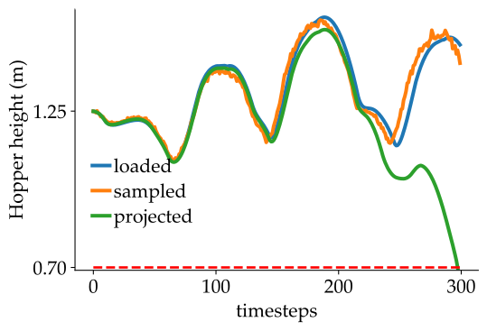
Fig. 3: Diverging projection of the Hopper height. Our diffusion model samples the orange trajectory given the initial state of the blue trajectory, which is loaded from our dataset. The projection of orange with Algorithm 1 yields the diverging but admissible green trajectory. However, green is not the admissible trajectory closest to orange since blue is admissible and much closer to orange than green.
Equation 6
𝒫ref​(s~t+1,𝒞⁡(st),st+1ref):=arg⁡minc∈𝒞⁡(st)​{‖s~t+1−c‖+λ​‖st+1ref−c‖},\mathcal{P}^{\text{ref}}\big(\tilde{s}_{t+1},\mathcal{C}(s_{t}),s_{t+1}^{\text{ref}}\big):=\underset{c\,\in\,\mathcal{C}(s_{t})}{\arg\min}\big\{\|\tilde{s}_{t+1}-c\|+\lambda\|s_{t+1}^{\text{ref}}-c\|\big\}, (6)
Algorithm 2 Reference Trajectory Projection
1: predicted trajectory τ~={s0,s~1,…​s~H}∈𝒮H+1\tilde{\tau}=\big\{s_{0},\tilde{s}_{1},...\tilde{s}_{H}\big\}\in\mathcal{S}^{H+1}, reference trajectory τref={s0,s1ref,…​sHref}∈𝒮H+1\tau^{\text{ref}}=\big\{s_{0},s_{1}^{\text{ref}},...s_{H}^{\text{ref}}\big\}\in\mathcal{S}^{H+1}.
2: τ={s0}\tau=\big\{s_{0}\big\} ⊳\triangleright initialize the projected trajectory
3: for t=0t=0 to H−1H-1 do
4:   𝒞⁡(st)=conv⁡(f⁡(st,v1),…,f⁡(st,vm))\mathcal{C}(s_{t})=\conv\big(f(s_{t},v_{1}),...,f(s_{t},v_{m})\big)
5:   st+1=𝒫ref​(s~t+1,𝒞⁡(st),st+1ref)s_{t+1}=\mathcal{P}^{\text{ref}}\big(\tilde{s}_{t+1},\mathcal{C}(s_{t}),s^{\text{ref}}_{t+1}\big) ⊳\triangleright next state projection
6:   τ←τ∪{st+1}\tau\leftarrow\tau\cup\{s_{t+1}\} ⊳\triangleright append to τ\tau
7: return τ\tau

IV-C Using action predictions for better state projections

Jointly predicted actions center a smaller action-search region before constructing the successor-state hull. Convex optimization then chooses weights for both an approximate next state and its associated action. Matching convex combinations of actions and successors is exact for control-affine dynamics; general nonlinear or contact dynamics can still produce a discrepancy. Restricting the search improves local precision but does not remove the exponential vertex cost.

Equations 7–8
v^i=a~t+δ⁡(vi−1m​∑i= 1mvi)\hat{v}_{i}=\tilde{a}_{t}+\delta\Big(v_{i}-\frac{1}{m}\sum_{i\,=\,1}^{m}v_{i}\Big) (7)
𝒞^​(st)=conv⁡(f⁡(st,v^1),…,f⁡(st,v^m))\hat{\mathcal{C}}(s_{t})=\conv\big(f(s_{t},\hat{v}_{1}),...,f(s_{t},\hat{v}_{m})\big) (8)
𝒜\mathcal{A}v1v_{1}v4v_{4}v2v_{2}v3v_{3}LLv^1\hat{v}_{1}v^4\hat{v}_{4}v^2\hat{v}_{2}v^3\hat{v}_{3}δ​L\delta La~t\tilde{a}_{t}𝒞⁡(st)\mathcal{C}(s_{t})f⁡(st,v1)f\!(\!s_{t},\!v_{1}\!)f⁡(st,v2)f\!(\!s_{t},\!v_{2}\!)f⁡(st,v3)f\!(\!s_{t},\!v_{3}\!)f⁡(st,v4)f\!(\!s_{t},\!v_{4}\!)𝒞^​(st)\hat{\mathcal{C}}(s_{t})f⁡(st,v^1)f\!(\!s_{t},\!\hat{v}_{1}\!)f⁡(st,v^2)f\!(\!s_{t},\!\hat{v}_{2}\!)f⁡(st,v^3)f\!(\!s_{t},\!\hat{v}_{3}\!)f⁡(st,v^4)f\!(\!s_{t},\!\hat{v}_{4}\!)
Fig. 4: Illustration of the reduced search space 𝒞^​(st)\hat{\mathcal{C}}(s_{t}) of (8) resulting from the reduced action space conv⁡(v^1,v^2,v^3,v^4)\conv(\hat{v}_{1},\hat{v}_{2},\hat{v}_{3},\hat{v}_{4}) of (7) by a factor δ\delta surrounding action prediction a~t\tilde{a}_{t}. Finding the best next state st+1s_{t+1} is much easier in the smaller set 𝒞^​(st)\hat{\mathcal{C}}(s_{t}) than in the larger 𝒞⁡(st)\mathcal{C}(s_{t}).
Equations 9–10
𝒫⁡(s~t+1,𝒞^​(st)):=arg⁡minc^∈𝒞^​(st)​‖s~t+1−c^‖=∑i= 1mλi∗​f​(st,v^i)\mathcal{P}\big(\tilde{s}_{t+1},\hat{\mathcal{C}}(s_{t})\big):=\underset{\hat{c}\,\in\,\hat{\mathcal{C}}(s_{t})}{\arg\min}\|\tilde{s}_{t+1}-\hat{c}\|=\sum_{i\,=\,1}^{m}\lambda_{i}^{*}f(s_{t},\hat{v}_{i}) (9)
λ∗=arg⁡minλi∈[0,1]{∥s~t+1−∑i= 1mλif(st,v^i)∥s.t.∑i= 1mλi=1}.\lambda^{*}=\underset{\lambda_{i}\,\in\,[0,1]}{\arg\min}\Bigg\{\Big\|\tilde{s}_{t+1}-\sum_{i\,=\,1}^{m}\lambda_{i}f(s_{t},\hat{v}_{i})\Big\|\ \text{s.t.}\ \sum_{i\,=\,1}^{m}\lambda_{i}=1\hskip-1.42262pt\Bigg\}. (10)
Algorithm 3 State Action Trajectory Projection
1: predicted trajectory τ~={s0,s~1,…​s~H}∈𝒮H+1\tilde{\tau}=\big\{s_{0},\tilde{s}_{1},...\tilde{s}_{H}\big\}\in\mathcal{S}^{H+1}, predicted actions α~={a~0,…,a~H−1}∈𝒜H\tilde{\alpha}=\big\{\tilde{a}_{0},...,\tilde{a}_{H-1}\big\}\in\mathcal{A}^{H}.
2: τ={s0}\tau=\big\{s_{0}\big\}, α={}\alpha=\{\} ⊳\triangleright initialize the projections
3: for t=0t=0 to H−1H-1 do
4:   for i=1i=1 to mm do
5:    v^i=a~t+δ⁡(vi−1m​∑vi)\hat{v}_{i}=\tilde{a}_{t}+\delta\big(v_{i}-\frac{1}{m}\sum v_{i}\big) ⊳\triangleright extremal actions   
6:   λ∗=\lambda^{*}= solve (10)
7:   st+1=∑λ∗​f​(st,v^)s_{t+1}=\sum\lambda^{*}f(s_{t},\hat{v}), at=∑λ∗​v^a_{t}=\sum\lambda^{*}\hat{v} ⊳\triangleright predictions
8:   τ←τ∪{st+1}\tau\leftarrow\tau\cup\{s_{t+1}\}, α←α∪{at}\alpha\leftarrow\alpha\cup\{a_{t}\} ⊳\triangleright append to τ\tau, α\alpha
9: return τ\tau, α\alpha

IV-D Using action predictions for admissible state prediction

The action projector replaces each state prediction with the simulator’s successor under the predicted action. A second variant adds a learned action correction based on the disagreement between the desired successor and the uncorrected rollout. Both construct dynamically consistent simulator trajectories when the applied actions respect their admissible set. This is a model-relative dynamics statement, not a guarantee of state safety, task completion, or simulation-to-real agreement; the displayed correction equation does not explicitly specify an action-clipping step.

Equations 11–12
𝒫A​(st,a~t):=f⁡(st,a~t).\mathcal{P}^{\text{A}}(s_{t},\tilde{a}_{t}):=f(s_{t},\tilde{a}_{t}). (11)
𝒫SA​(st,a~t,s~t+1):=f⁡(st,a~t+δ​at).\mathcal{P}^{\text{SA}}(s_{t},\tilde{a}_{t},\tilde{s}_{t+1}):=f(s_{t},\tilde{a}_{t}+\delta a_{t}). (12)
min𝜃​𝔼δ​at∼𝒩⁡(0,σ2​I)​𝔼(st,at,st+1)∼𝒟​‖πθ​(st+1δ−st+1)−δ​at‖2.\underset{\theta}{\min}\underset{\delta a_{t}\sim\mathcal{N}(0,\sigma^{2}I)}{\mathbb{E}}\ \underset{(s_{t},a_{t},s_{t+1})\sim\mathcal{D}}{\mathbb{E}}\big\|\pi_{\theta}\big(s^{\delta}_{t+1}-s_{t+1}\big)-\delta a_{t}\big\|^{2}.
sts_{t}s~t+1\tilde{s}_{t+1}𝒫A\mathcal{P}^{\text{A}}a~t\tilde{a}_{t}𝒫SA\mathcal{P}^{\text{SA}}a~t+δ​at\tilde{a}_{t}+\delta a_{t}−\boldsymbol{-}+\boldsymbol{+}πθ\pi_{\theta}
Fig. 5: Illustration of projectors 𝒫A=f⁡(st,a~t){\color[rgb]{0.3,0.3,1}\mathcal{P}^{\text{A}}}=f(s_{t},{\color[rgb]{0.3,0.3,1}\tilde{a}_{t}}) and 𝒫SA=f⁡(st,a~t+δ​at){\color[rgb]{0,0.7,0}\mathcal{P}^{\text{SA}}}=f(s_{t},{\color[rgb]{0,0.7,0}\tilde{a}_{t}+\delta a_{t}}) with its feedback correction policy πθ\pi_{\theta} leveraging the open-loop error to generate a corrective action δ​at\delta a_{t} instead of discarding prediction s~t+1\tilde{s}_{t+1} like 𝒫A{\color[rgb]{0.3,0.3,1}\mathcal{P}^{\text{A}}}.

V Incorporating Projections in Diffusion

DDAT applies the selected correction within denoising and optionally within training. A noise-dependent schedule postpones strong corrections until the proposed trajectory contains meaningful structure. The experiments separately test the value of timing, training-time correction, and output modality.

V-A Training with projections

The proposed training loss compares a projected denoised sample with its demonstrated target, while inference alternates denoising, initial-state conditioning, and projection. Reference projection uses demonstrations during training but the unprojected generated sequence during inference. Differentiable optimization layers provide part of the gradient path, although the black-box simulator interrupts exact backpropagation. The later ablation does not support the hoped-for benefit of training with projection.

Algorithm 4 DDAT

Training

1: dataset of trajectories 𝒟\mathcal{D}, projector 𝒫σ\mathcal{P}_{\sigma} of (5), (6), (11), or (12).
2: while not converged do
3:   σ∼exp⁡(𝒩⁡(pm,ps2))\sigma\sim\exp\big(\mathcal{N}(p_{m},p_{s}^{2})\big) ⊳\triangleright noise level, Appendix C.
4:   ε∼𝒩⁡(0,σ2​I)\varepsilon\sim\mathcal{N}(0,\sigma^{2}I) ⊳\triangleright noise sequence
5:   τ∼𝒰⁡(𝒟)\tau\sim\mathcal{U}(\mathcal{D}) ⊳\triangleright training trajectory
6:   τ~←Dθ​(τ+ε,σ)\tilde{\tau}\leftarrow D_{\theta}(\tau+\varepsilon;\ \sigma) ⊳\triangleright denoised prediction
7:   τ~←𝒫σ​(τ~)\tilde{\tau}\leftarrow\mathcal{P}_{\sigma}\big(\tilde{\tau}\big) ⊳\triangleright projection
8:   ℒ=‖τ~−τ‖2\mathcal{L}=\|\tilde{\tau}-\tau\|^{2} ⊳\triangleright loss
9:   θ←θ−∇θℒ\theta\leftarrow\theta-\nabla_{\theta}\mathcal{L} ⊳\triangleright gradient step

Inference

1: initial state s0s_{0}.
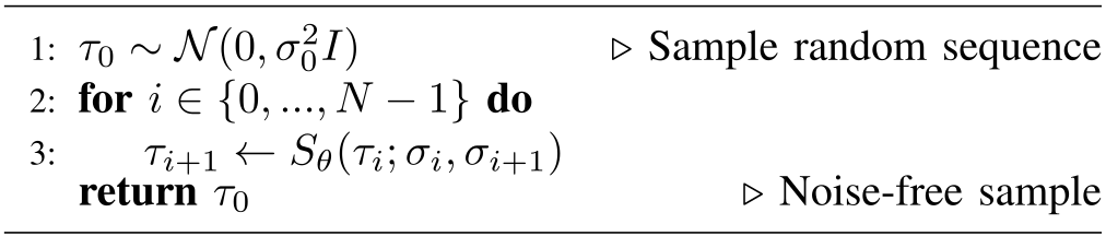
2: τ0∼𝒩⁡(0,σ02​I)\tau_{0}\sim\mathcal{N}\big(0,\sigma_{0}^{2}I\big) ⊳\triangleright initialize trajectory
3: τ0​[0]←s0\tau_{0}[0]\leftarrow s_{0} ⊳\triangleright known initial state
4: for i=0i=0 to N−1N-1 do
5:   τi+1←Sθ​(τi,σi,σi+1)\tau_{i+1}\leftarrow S_{\theta}(\tau_{i};\sigma_{i},\sigma_{i+1}) ⊳\triangleright denoised prediction (2)
6:   τi+1​[0]←s0\tau_{i+1}[0]\leftarrow s_{0} ⊳\triangleright known initial state
7:   τi+1←𝒫σi​(τi+1)\tau_{i+1}\leftarrow\mathcal{P}_{\sigma_{i}}\big(\tau_{i+1}\big) ⊳\triangleright projection
8: return τN\tau_{N} ⊳\triangleright noise-free sample

V-B Projection curriculum

The curriculum skips projection at high noise, gradually increases its probability in a transition band, and projects every transition at low noise. The Bernoulli variable in the displayed formula marks skipping, so the projection probability is one minus the displayed probability. Partial intermediate projection breaks some chains of accumulated error, while the final low-noise stage restores correction at every transition. This is a stabilization strategy whose empirical value is tested separately.

Equation
𝒫σ​(s~t+1,⋅):=(1−b)​𝒫​(s~t+1,⋅)+b​s~t+1​with​b∼ℬ⁡(p⁡(σ)),\displaystyle\mathcal{P}_{\sigma}(\tilde{s}_{t+1},\cdot):=(1-b)\mathcal{P}(\tilde{s}_{t+1},\cdot)+b\tilde{s}_{t+1}\hskip 5.69054pt\text{with}\hskip 5.69054ptb\sim\mathcal{B}\big(p(\sigma)\big),
where​p​(σ):={1if​σ>σmax,σ−σminσmax−σminif​σ∈[σmin,σmax],0if​σ<σmin,\displaystyle\text{where}\hskip 5.69054ptp(\sigma):=\left\{\begin{array}[]{ll}1&\text{if}\ \sigma>\sigma_{\text{max}},\\ \displaystyle\frac{\sigma-\sigma_{\text{min}}}{\sigma_{\text{max}}-\sigma_{\text{min}}}&\text{if}\ \sigma\in[\sigma_{\text{min}},\sigma_{\text{max}}],\\ 0&\text{if}\ \sigma<\sigma_{\text{min}},\end{array}\right.

VI Implementation

Experiments compare state-only, action-only, and joint models with several correction variants. Evaluation includes both model-relative admissibility and useful behavior, since a perfectly consistent rollout can still fall, miss a target, or receive poor reward.

VI-A Test environments

The environments are Hopper, Walker, HalfCheetah, a custom quadcopter, and Unitree GO1 and GO2 quadrupeds. State dimensions range from twelve to thirty-seven and action dimensions from three to twelve. Demonstrations come from simulated control policies; these datasets are constructed for reproducibility rather than taken unchanged from a standard offline benchmark.

VI-B Diffusion architecture

A diffusion transformer models sequences. Convex layers differentiate the optimization parts of projection, but simulator calls prevent complete gradients through the correction. Inference generates a batch and chooses a trajectory using a task criterion, often predicted time before falling. Reported behavior therefore includes candidate sampling and selection, despite the introduction’s motivation to reduce reliance on large batches.

VI-C Evaluation metrics

Statewise admissibility error measures each proposed transition’s distance from a simulator successor found by inverse dynamics. Cumulative error recursively rolls out such recovered actions and measures divergence from the proposed sequence. The numerical inverse solver limits their precision; its greedy recursion is not a proof of the globally nearest admissible trajectory. Model labels record state/action outputs, projector type, curriculum, inference-only use, and conditioning. Rewards and survival are separate outcome measures.

Equations 16–18
I​D​(st,st+1):=arg⁡mina∈𝒜​{‖st+1−f⁡(st,a)‖},I\!D(s_{t},s_{t+1}):=\underset{a\,\in\,\mathcal{A}}{\arg\min}\big\{\big\|s_{t+1}-f(s_{t},a)\big\|\big\}, (16)
S​A​E​(st,s~t+1):=‖s~t+1−f⁡(st,I​D​(st,s~t+1))‖.SAE(s_{t},\tilde{s}_{t+1}):=\big\|\tilde{s}_{t+1}-f\big(s_{t},I\!D(s_{t},\tilde{s}_{t+1})\big)\big\|. (17)
C​A​E​(τ~):=‖{s~1,…,s~H}−{s1,…,sH}‖,CAE(\tilde{\tau}):=\big\|\big\{\tilde{s}_{1},...,\tilde{s}_{H}\big\}-\big\{s_{1},...,s_{H}\big\}\big\|, (18)

VII Experiments

The experiments ask whether projections improve consistency, when they should occur, whether they should be included during training, and which prediction modality works best. The retained tables and plots preserve the different sample counts, uncertainty summaries, and evaluation domains.

VII-A Generating admissible trajectories

All tested projection schemes reduce measured statewise and cumulative error relative to unprojected state plans. Direct action-rollout projectors have zero simulator consistency error by construction, which does not imply zero tracking error on hardware. Other variants remain limited by convex approximations and the evaluation inverse solver. Particularly precise inverse dynamics are needed for HalfCheetah and the quadcopter; state-only quadruped evaluation is unavailable.

System Model SAE (↓\downarrow) CAE (↓\downarrow)
Hopper SS 1.1​e−11.1\text{e}{-1} 1.71.7
S​𝒫IS\mathcal{P}_{I} 8.5​e−38.5\text{e}{-3} 4.8​e−14.8\text{e}{-1}
S​A​𝒫ISA\mathcal{P}_{I} 4.2​e−44.2\text{e}{-4} 6.5​e−26.5\text{e}{-2}
S​𝒫σrefS\mathcal{P}_{\sigma}^{\text{ref}} 7.5​e−37.5\text{e}{-3} 6.4​e−16.4\text{e}{-1}
S​A​𝒫σA, SASA\mathcal{P}_{\sigma}^{\text{A, SA}} 𝟎\mathbf{0} 𝟎\mathbf{0}
I​DI\!D 6.9​e−56.9\text{e}{-5} 9.5​e−49.5\text{e}{-4}
Walker S​ASA 3.1​e−13.1\text{e}{-1} 3.93.9
S​A​𝒫ISA\mathcal{P}_{I} 5.4​e−45.4\text{e}{-4} 3.5​e−13.5\text{e}{-1}
S​A​𝒫σrefSA\mathcal{P}_{\sigma}^{\text{ref}} 7.1​e−47.1\text{e}{-4} 3.5​e−13.5\text{e}{-1}
S​A​𝒫σA, SASA\mathcal{P}_{\sigma}^{\text{A, SA}} 𝟎\mathbf{0} 𝟎\mathbf{0}
I​DI\!D 1.3​e−51.3\text{e}{-5} 6.2​e−26.2\text{e}{-2}
HalfCheetah S​ASA 2.8​e−12.8\text{e}{-1} 4.64.6
S​A​𝒫ISA\mathcal{P}_{I} 4.8​e−34.8\text{e}{-3} 1.991.99
S​A​𝒫σrefSA\mathcal{P}_{\sigma}^{\text{ref}} 4.4​e−44.4\text{e}{-4} 2.12.1
S​A​𝒫σA, SASA\mathcal{P}_{\sigma}^{\text{A, SA}} 𝟎\mathbf{0} 𝟎\mathbf{0}
I​DI\!D 5.5​e−125.5\text{e}{-12} 3.1​e−23.1\text{e}{-2}
Quadcopter SS 2.55​e−12.55\text{e}{-1} 9.57​e−19.57\text{e}{-1}
S​𝒫σrefS\mathcal{P}_{\sigma}^{\text{ref}} 4.77​e−44.77\text{e}{-4} 4.88​e−44.88\text{e}{-4}
S​ASA 3.24​e−13.24\text{e}{-1} 1.481.48
S​A​𝒫σrefSA\mathcal{P}_{\sigma}^{\text{ref}} 1.22​e−61.22\text{e}{-6} 1.68​e−51.68\text{e}{-5}
S​A​𝒫σA,S​ASA\mathcal{P}_{\sigma}^{A,SA} 𝟎\mathbf{0} 𝟎\mathbf{0}
I​DI\!D 1.14​e−171.14\text{e}{-17} 1.04​e−161.04\text{e}{-16}
TABLE I: Distance to admissibility of 100100 trajectories generated by diffusion models. The errors are calculated with the inverse dynamics models (I​DI\!D) whose precision limit that of the models. Applying any projection scheme decreases the admissibility errors by orders of magnitude on all robots.

VII-B Projection curriculum during inference

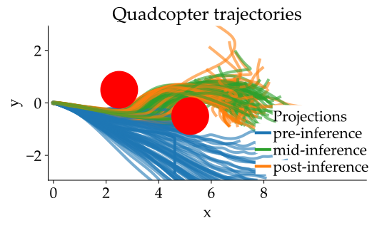
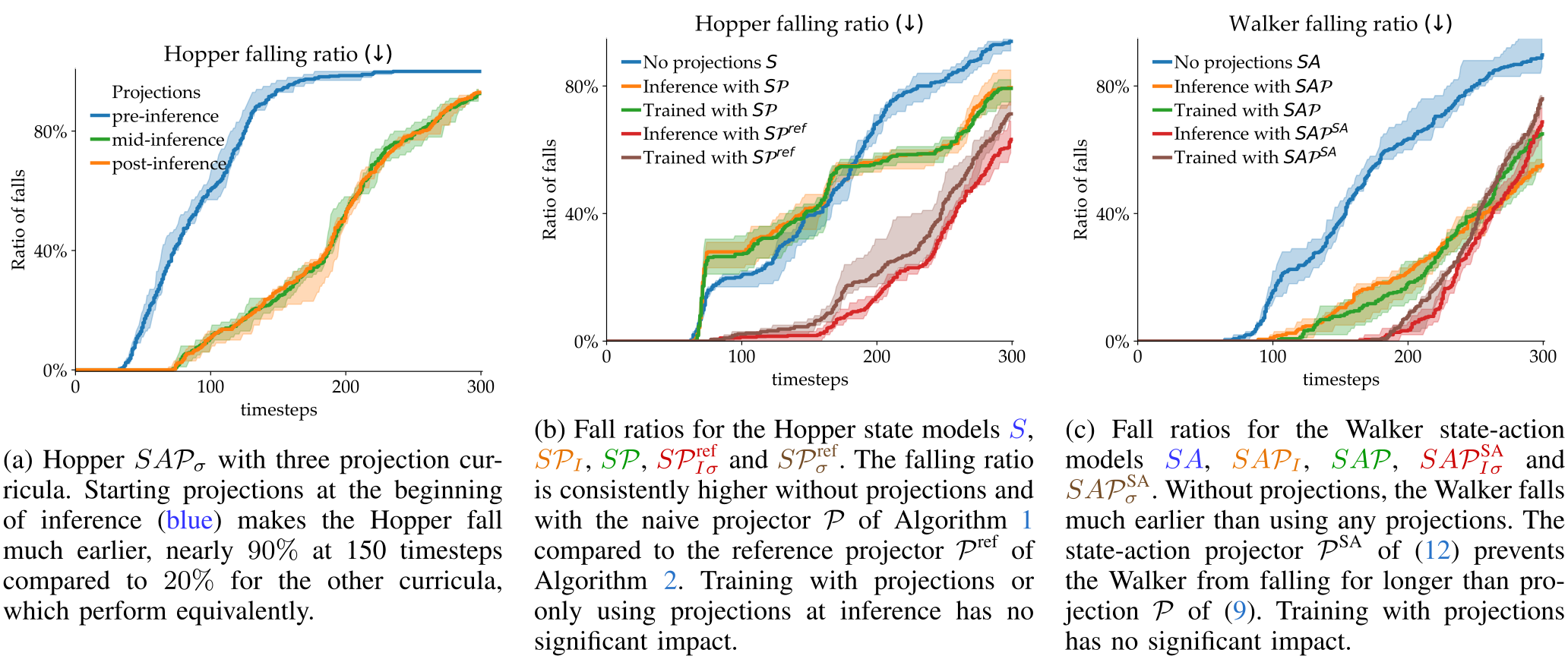
Projecting from the highest-noise step harms behavioral quality. In the quadcopter slalom illustration, no early-projection samples pass both obstacles, compared with 81% and 79% for middle and final projection. The corresponding table reports similar admissibility and no significant difference between middle and final schedules. Avoiding high-noise correction is supported more strongly than a claim that the gradual curriculum always beats a final projection.
Original compound figure with every panel and label in the source arrangement.
Fig. 6: Ratios of trajectories deployed open-loop having fallen at a given timestep for the Hopper and Walker. The shade is the maximum and minimum number of trajectories having fallen at each timestep over 5 runs of 100 trajectories each.
parameters Hopper S​A​𝒫σSA\mathcal{P}_{\sigma} Quadcopter S​A​𝒫σSASA\mathcal{P}_{\sigma}^{\text{SA}}
Model σm​i​n\sigma_{min} σm​a​x\sigma_{max} SAE (↓\downarrow) CAE (↓\downarrow) survival% (↑\uparrow) reward (↑\uparrow) survival% (↑\uparrow) reward (↑\uparrow)
pre 8080 8080 4.92​e−44.92\text{e}{-4} 5.57​e−25.57\text{e}{-2} 27±1027\pm 10 131±46131\pm 46 85±2085\pm 20 16±1416\pm 14
mid 0.00210.0021 0.20.2 1.41​e−𝟒\mathbf{1.41\text{e}{-4}} 6.13​e−26.13\text{e}{-2} 𝟔𝟓±𝟐𝟏\mathbf{65\pm 21} 𝟑𝟔𝟒±𝟏𝟑𝟎\mathbf{364\pm 130} 𝟗𝟎±𝟐𝟏\mathbf{90\pm 21} 𝟗𝟑±𝟑𝟒\mathbf{93\pm 34}
post 0.00210.0021 0.00210.0021 1.45​e−41.45\text{e}{-4} 4.82​e−𝟐\mathbf{4.82\text{e}{-2}} 63±2463\pm 24 345±152345\pm 152 𝟗𝟎±𝟐𝟏\mathbf{90\pm 21} 𝟗𝟑±𝟑𝟒\mathbf{93\pm 34}
TABLE II: Distance to admissibility of generated trajectories projected either at each step of inference (pre), gradually during inference (mid), or only after inference (post). The results are averaged over 500 trajectories and clearly demonstrate that projections at high noise level (pre) hurt significantly the quality of the trajectories in terms of survival and reward. The admissibility is only marginally affected by the projection curriculum. The difference between post-inference projections and mid-inference projections is not significant. The Quadcopter trajectories are projected with S​A​𝒫σSASA\mathcal{P}_{\sigma}^{\text{SA}} and hence are all admissible.
Original figure
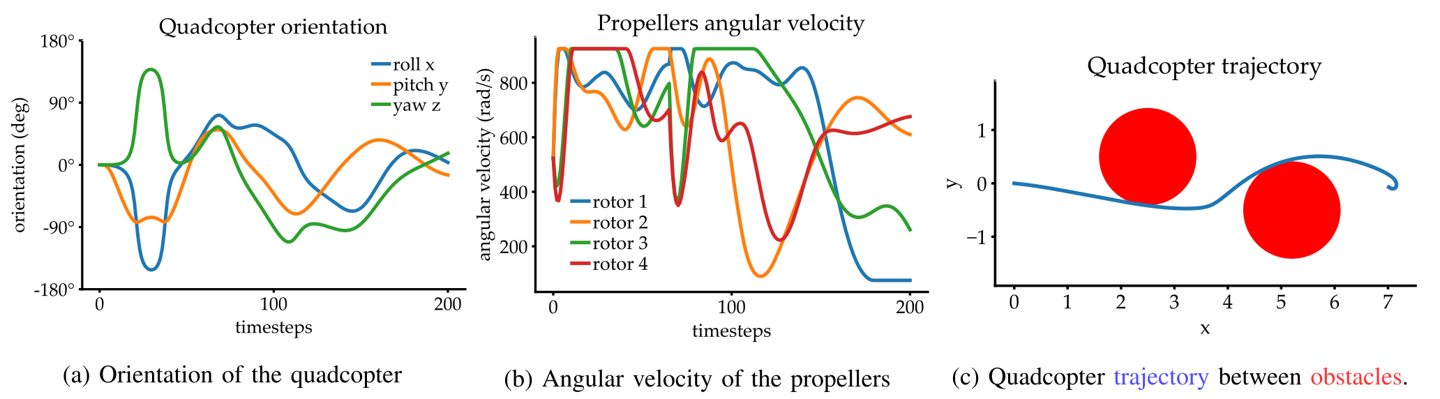
Fig. 7: Quadcopter trajectories generated by the S​A​𝒫σSASA\mathcal{P}_{\sigma}^{\text{SA}} model with projections starting either pre-inference, or mid-inference or post-inference. The desired behavior exhibited in Fig. 9(c) slaloms between the obstacles. None of the trajectories generated by the pre-inference model pass the obstacles, whereas 81%81\% and 79%79\% of the trajectories generated by the other two projection curricula pass the slalom. Hence, projections at the beginning of inference strongly reduce the quality of the samples.

VII-C Training with projections

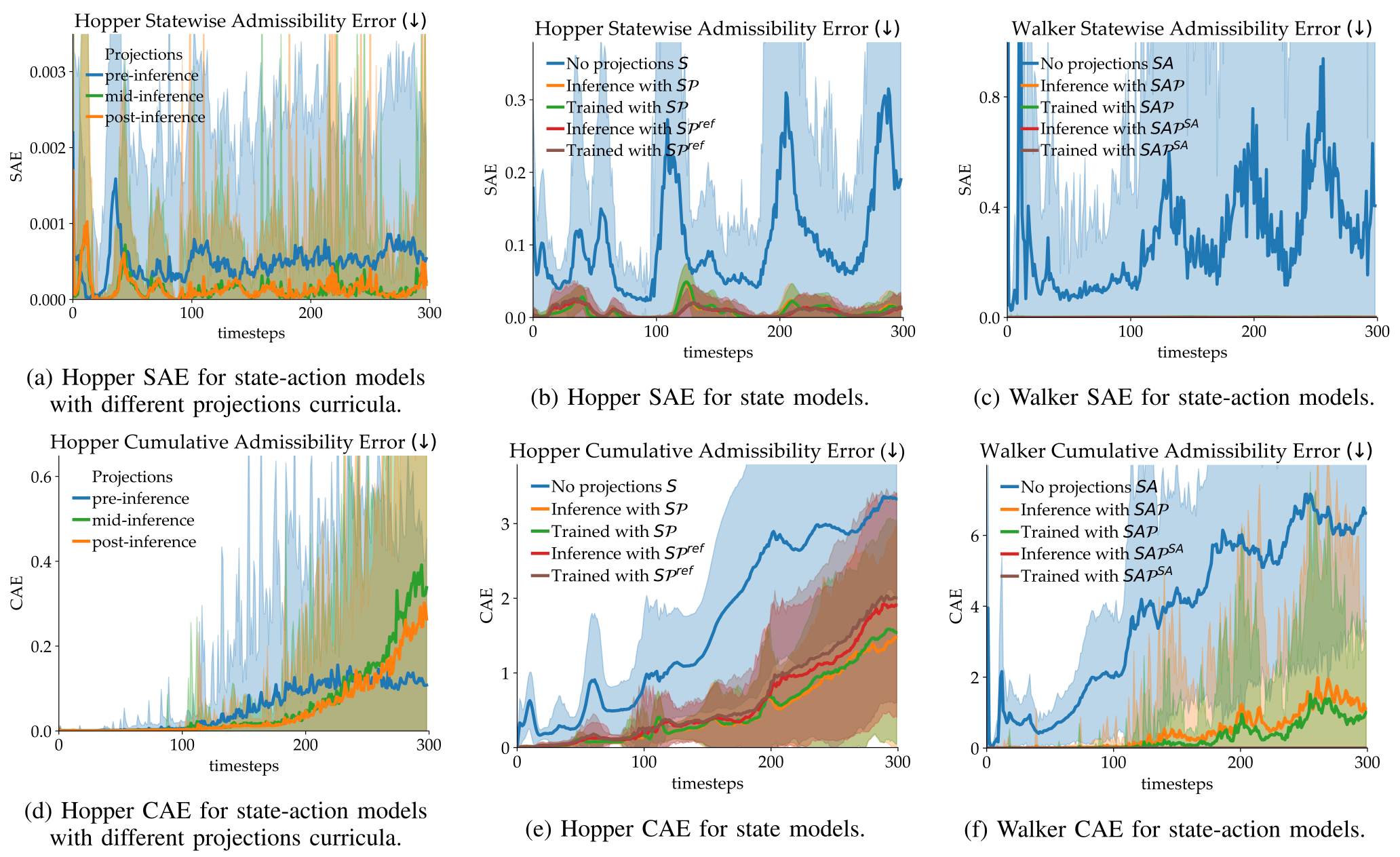
The training ablation is negative: adding projections during training provides little or no significant improvement in either trajectory quality or admissibility over inference-only projection. The larger differences come from projector choice. Corrections still increase and destabilize training loss despite the proposed curriculum. This finding qualifies the training-time projection contribution emphasized in the introduction.
Original compound figure with every panel and label in the source arrangement.
Fig. 8: Statewise (SAE) and Cumulative (CAE) Admissibility Errors for different Hopper and Walker models collected over 5 runs of 100 initial conditions with 8 samples each. The shade shows the standard deviation. Figures (8(b)) (8(c)), (8(e)) and (8(f)) show that projections drastically improve the admissibility of models. Figures (8(a)) and (8(d)) show small difference in admissibility when projecting during inference

VII-D Diffusion modality

Joint state–action models with corrected rollouts perform consistently well, but they do not win every metric. State-only reference projection is strongest on the reported Hopper comparison; action-only planning is competitive on HalfCheetah and gives the highest GO1 reward, yet performs less well on GO2. The action-only baseline adapts the policy component of D-MPC to the authors’ data and transformer, not its full learned-model system. Dataset controllers use closed-loop feedback, so their stronger results are not an equal open-loop comparison.

Model Hopper Walker HalfCheetah Quadcopter
survival (↑\uparrow) reward (↑\uparrow) survival (↑\uparrow) reward (↑\uparrow) survival (↑\uparrow) reward (↑\uparrow) survival (↑\uparrow) reward (↑\uparrow)
MPPI [48] 10±310\pm 3 85±5985\pm 59 0±00\pm 0 1±61\pm 6 0±00\pm 0 −33±37-33\pm 37 0±00\pm 0 −639±225-639\pm 225
data 100±0100\pm 0 563±21563\pm 21 100±0100\pm 0 995±80995\pm 80 100±0100\pm 0 611±30611\pm 30 100±0100\pm 0 117±5.7117\pm 5.7
S​ASA 50±2550\pm 25 294±190294\pm 190 58±2258\pm 22 333±184333\pm 184 87±1587\pm 15 226±88226\pm 88 65±3165\pm 31 32±2832\pm 28
S​A​𝒫ISA\mathcal{P}_{I} 67±2267\pm 22 369±141369\pm 141 84±1884\pm 18 516±177516\pm 177 94±1094\pm 10 318±104318\pm 104 66±2966\pm 29 43±2843\pm 28
S​A​𝒫σrefSA\mathcal{P}_{\sigma}^{\text{ref}} 𝟕𝟐±𝟏𝟗\mathbf{72\pm 19} 𝟒𝟏𝟎±𝟏𝟓𝟑\mathbf{410\pm 153} 83±1183\pm 11 430±218430\pm 218 94±1094\pm 10 314±102314\pm 102 60±2960\pm 29 34±2434\pm 24
S​A​𝒫σSASA\mathcal{P}_{\sigma}^{\text{SA}} 𝟕𝟐±𝟏𝟗\mathbf{72\pm 19} 371±112371\pm 112 𝟖𝟔±𝟏𝟑\mathbf{86\pm 13} 𝟔𝟐𝟎±𝟏𝟗𝟓\mathbf{620\pm 195} 𝟏𝟎𝟎±𝟎\mathbf{100\pm 0} 353±69353\pm 69 𝟖𝟕±𝟐𝟑\mathbf{87\pm 23} 𝟗𝟎±𝟑𝟖\mathbf{90\pm 38}
S​A​𝒫σASA\mathcal{P}_{\sigma}^{\text{A}} 13±713\pm 7 51±3351\pm 33 82±1482\pm 14 285±148285\pm 148 97±797\pm 7 𝟒𝟎𝟒±𝟖𝟑\mathbf{404\pm 83} 76±2976\pm 29 25±2025\pm 20
A(⋅|s0)A(\cdot|s_{0}) 25±1125\pm 11 120±65120\pm 65 71±2371\pm 23 494±181494\pm 181 99±399\pm 3 395±94395\pm 94 78±2578\pm 25 61±3261\pm 32
TABLE III: Mean and standard deviation of reward and survival rates (%) over 100 initial states with 8 trajectories sampled for each. As in [20] we used Model Predictive Path Integral (MPPI) [48] as a baseline, but it struggled due to the long-horizon nature of our tasks. The data row refers to our training data generated by closed-loop RL or MPC policies, which is why their performance exceeds all the open-loop models. Among all the models tested S​A​𝒫σSASA\mathcal{P}^{\text{SA}}_{\sigma} consistently perform among the best.
System Model survival % (↑\uparrow) reward (↑\uparrow)
Hopper S​𝒫σrefS\mathcal{P}_{\sigma}^{\text{ref}} 𝟖𝟖±𝟏𝟔\mathbf{88\pm 16} 𝟓𝟏𝟗±𝟏𝟑𝟎\mathbf{519\pm 130}
S​A​𝒫σSASA\mathcal{P}_{\sigma}^{\text{SA}} 72±1972\pm 19 371±112371\pm 112
A(⋅|s0)A(\cdot|s_{0}) 25±1125\pm 11 120±65120\pm 65
Walker S​𝒫σrefS\mathcal{P}_{\sigma}^{\text{ref}} 63±2363\pm 23 365±134365\pm 134
S​A​𝒫σSASA\mathcal{P}_{\sigma}^{\text{SA}} 𝟖𝟔±𝟏𝟑\mathbf{86\pm 13} 𝟔𝟐𝟎±𝟏𝟗𝟓\mathbf{620\pm 195}
A(⋅|s0)A(\cdot|s_{0}) 71±2371\pm 23 494±181494\pm 181
HalfCheetah S​A​𝒫σSASA\mathcal{P}_{\sigma}^{\text{SA}} 𝟏𝟎𝟎±𝟎\mathbf{100\pm 0} 353±69353\pm 69
A(⋅|s0)A(\cdot|s_{0}) 99±399\pm 3 𝟑𝟗𝟓±𝟗𝟒\mathbf{395\pm 94}
Quadcopter S​𝒫σrefS\mathcal{P}_{\sigma}^{\text{ref}} 𝟖𝟗±𝟏𝟗\mathbf{89\pm 19} 89±3389\pm 33
S​A​𝒫σSASA\mathcal{P}_{\sigma}^{\text{SA}} 87±2387\pm 23 𝟗𝟎±𝟑𝟖\mathbf{90\pm 38}
A(⋅|s0)A(\cdot|s_{0}) 78±2578\pm 25 61±3261\pm 32
TABLE IV: Reward and survival comparison between S, SA, and A models averaged over 100 initial states and 8 trajectories generated for each. We could not evaluate state models for the HalfCheetah due to the lack of performant inverse dynamics model. Despite their lack of admissibility guarantees state models perform well on the Hopper and Quadcopter. State-action model S​A​𝒫σSASA\mathcal{P}_{\sigma}^{\text{SA}} is consistently near the best while action models A(⋅|s0)A(\cdot|s_{0}) achieve inconsistent results.
System Model survival (↑\uparrow) reward (↑\uparrow)
Unitree GO1 SA(⋅|c)SA(\cdot|c) 87±2587\pm 25 653±408653\pm 408
SA𝒫σSA(⋅|c)SA\mathcal{P}^{\text{SA}}_{\sigma}(\cdot|c) 87±2887\pm 28 638±409638\pm 409
SA𝒫σA(⋅|c)SA\mathcal{P}^{\text{A}}_{\sigma}(\cdot|c) 𝟏𝟎𝟎±𝟎\mathbf{100\pm 0} 818±466818\pm 466
A(⋅|c,s0)A(\cdot|c,s_{0}) 99±399\pm 3 𝟏𝟎𝟖𝟏±𝟒𝟗𝟓\mathbf{1081\pm 495}
Unitree GO2 SA(⋅|c)SA(\cdot|c) 𝟏𝟎𝟎±𝟎\mathbf{100\pm 0} 1039±1221039\pm 122
SA𝒫σSA(⋅|c)SA\mathcal{P}^{\text{SA}}_{\sigma}(\cdot|c) 𝟏𝟎𝟎±𝟎\mathbf{100\pm 0} 𝟏𝟎𝟖𝟎±𝟑𝟓\mathbf{1080\pm 35}
SA𝒫σA(⋅|c)SA\mathcal{P}^{\text{A}}_{\sigma}(\cdot|c) 𝟏𝟎𝟎±𝟎\mathbf{100\pm 0} 1074±531074\pm 53
A(⋅|c,s0)A(\cdot|c,s_{0}) 𝟏𝟎𝟎±𝟎\mathbf{100\pm 0} 911±217911\pm 217
TABLE V: Reward and survival rates (%) ±s​t​d\pm std over 100 initial states s0s_{0} with 64 samples generated per s0s_{0}. All these models predict actions implemented open-loop on the robots and conditioned on the velocity command cc. We could not evaluate state models for the Unitree due to the lack of performant inverse dynamics model. The action only model A(⋅|c,s0)A(\cdot|c,s_{0}) ranks respectively best and worse on the GO1 and GO2, whereas state-action model SA𝒫σA(⋅|c)SA\mathcal{P}^{\text{A}}_{\sigma}(\cdot|c) performs consistently well on both robots.

VIII Hardware Experiments

Thirty GO2 trials per method repeat three sampled ten-second trajectories ten times each. DDAT succeeds in 23/30 trials, with five region exits and two falls, versus 10/30 successes, sixteen exits, and four falls for the unprojected baseline. Thus the sixty trials are not sixty independently sampled plans. The task is a three-meter straight walk in a prescribed corridor; onboard recovery and physical variability affect failures. A separate GO1 demonstration walks two meters with 0.32 meters of lateral deviation. These results support this constrained open-loop setting, not general robust locomotion.

Model Success (↑\uparrow) Exits (↓\downarrow) Falls (↓\downarrow)
SA𝒫σSA(⋅,|c)SA\mathcal{P}_{\sigma}^{\text{SA}}(\cdot,|c) 𝟐𝟑/𝟑𝟎\mathbf{23/30} 𝟓/𝟑𝟎\mathbf{5/30} 𝟐/𝟑𝟎\mathbf{2/30}
SA(⋅,|c)SA(\cdot,|c) 10/3010/30 16/3016/30 4/304/30
TABLE VI: Evaluation of 6060 walking hardware trials of trajectories generated by diffusion models on the Unitree GO2. If the quadruped ever left the prescribed region (Exits) or lost balance to the point of falling, we considered the runs as failures.

IX Limitations

Admissibility verification assumes an accurate simulator. Learning a model could remove that access requirement and permit fuller differentiation, but would introduce model error and is proposed future work. Training remains expensive, and even five denoising steps can be slow when projections require sequential simulation and convex optimization. High-dimensional action sets and long horizons exacerbate that cost.

X Conclusion and Future Work

The principal practical result is that dynamics-aware correction can improve open-loop diffusion plans, particularly when joint predictions are converted into simulator rollouts. The experiments favor suitable projection choice and avoiding high-noise correction, while finding no clear benefit from projection during training. Faster closed-loop deployment and learned dynamics without simulator access remain future directions.

Acknowledgments

The authors acknowledge public and industrial research support and shared quadcopter/controller code. Koushil Sreenath discloses a financial interest in the Robotics and AI Institute and potential benefit from commercialization. These statements provide the paper’s original funding and conflict-of-interest context.

Appendix A Projection of actuated states

Known state meanings and numerical integration rules can eliminate dependent coordinates from the projection optimization. For explicit Euler, current position and velocity determine the next position; semi-implicit Euler links it to the next velocity. Optimizing only necessary velocity components produced comparable quality more quickly, while position-based projection diverged faster in the reported experiments. This reduction uses structural knowledge beyond merely calling an unlabeled simulator.

Equation 19
𝒫⁡(s~t+1,𝒞⁡(st)):=(xt+d​t​vt,arg⁡minr∈ℛ​‖v~t+1−r‖),\mathcal{P}\big(\tilde{s}_{t+1},\mathcal{C}(s_{t})\big):=\big(x_{t}+dt\,v_{t}\,,\ \underset{r\,\in\,\mathcal{R}}{\arg\min}\|\tilde{v}_{t+1}-r\|\big), (19)

Appendix B Inverse Dynamics

Inverse dynamics is a numerical verification tool. A convex-combination search works especially well for control-affine dynamics, while random directional search and line search refine more difficult cases. Even the combination lacks adequate precision or speed for some systems; twelve action dimensions require 4,096 hyperrectangle vertices. The recursive verifier supplies a feasible comparison rollout rather than a certified global nearest trajectory. All three original algorithms and the control-affine derivation are retained.

Algorithm 5 Trajectory Inverse Dynamics
1: predicted trajectory τ~={s0,s~1,…​s~H}∈𝒮H+1\tilde{\tau}=\big\{s_{0},\tilde{s}_{1},...\tilde{s}_{H}\big\}\in\mathcal{S}^{H+1}.
2: τ={s0}\tau=\big\{s_{0}\big\} ⊳\triangleright initialize the admissible trajectory
3: for t=0t=0 to H−1H-1 do
4:   at=I​D​(st,s~t+1)a_{t}=I\!D\big(s_{t},\tilde{s}_{t+1}\big) ⊳\triangleright best action
5:   st+1=f⁡(st,at)s_{t+1}=f\big(s_{t},a_{t}\big) ⊳\triangleright closest admissible next state
6:   τ←τ∪{st+1}\tau\leftarrow\tau\cup\{s_{t+1}\} ⊳\triangleright append to τ\tau
7: return τ\tau
8: admissibility of τ\tau.
Equation
s~\displaystyle\tilde{s} =∑λi​si=∑λi​g​(st)+λi​h​(st)​ai\displaystyle=\sum\lambda_{i}s^{i}=\sum\lambda_{i}g(s_{t})+\lambda_{i}h(s_{t})a^{i}
=g⁡(st)​∑λi+h⁡(st)​∑λi​ai=g⁡(st)+h⁡(st)​a~.\displaystyle=g(s_{t})\sum\lambda_{i}+h(s_{t})\sum\lambda_{i}a^{i}=g(s_{t})+h(s_{t})\tilde{a}.
Algorithm 6 Inverse Dynamics by Polytopic Optimization
1: current state st∈𝒮s_{t}\in\mathcal{S}, predicted next state s~t+1∈𝒮\tilde{s}_{t+1}\in\mathcal{S}.
2: a=1m​∑i=1mvia=\frac{1}{m}\sum_{i=1}^{m}v_{i} ⊳\triangleright initial guess, if not provided
3: st+1=f⁡(st,a)s_{t+1}=f(s_{t},a) ⊳\triangleright admissible next state
4: n=0n=0
5: while n<Nn<N and ‖s~t+1−st+1‖>ε\|\tilde{s}_{t+1}-s_{t+1}\|>\varepsilon do
6:   for i=1i=1 to mm do
7:    v^i=a+δ⁡(vi−1m​∑vi)\hat{v}_{i}=a+\delta\big(v_{i}-\frac{1}{m}\sum v_{i}\big) ⊳\triangleright extremal actions
8:    si=f⁡(st,v^i)s^{i}=f(s_{t},\hat{v}_{i}) ⊳\triangleright extremal next states   
9:   λ∗=\lambda^{*}= solve (10)
10:   a=∑i=1mλi∗​v^ia=\sum_{i=1}^{m}\lambda_{i}^{*}\hat{v}_{i} ⊳\triangleright update the action
11:   st+1=f⁡(st,a)s_{t+1}=f(s_{t},a) ⊳\triangleright admissible next state
12:   n←n+1n\leftarrow n+1
13: Admissible next state st+1s_{t+1} is as close as possible to prediction s~t+1\tilde{s}_{t+1}
Algorithm 7 Inverse Dynamics by Black-Box Optimization
1: current state st∈𝒮s_{t}\in\mathcal{S}, predicted next state s~t+1∈𝒮\tilde{s}_{t+1}\in\mathcal{S}
2: a∼𝒰⁡(𝒜)a\sim\mathcal{U}\big(\mathcal{A}\big) ⊳\triangleright initial guess, if not provided
3: st+1=f⁡(st,a)s_{t+1}=f(s_{t},a) ⊳\triangleright admissible next state
4: n=0n=0
5: while n<Nn<N and ‖s~t+1−st+1‖>ε\|\tilde{s}_{t+1}-s_{t+1}\|>\varepsilon do
6:   δ​a∼𝒩⁡(0,σ)\delta a\sim\mathcal{N}(0,\sigma) with σ\sigma proportional to ‖s~−s′‖\|\tilde{s}-s^{\prime}\|
7:   if ‖s~−s′‖>‖s~−f⁡(s,a+δ​a)‖\|\tilde{s}-s^{\prime}\|>\|\tilde{s}-f(s,a+\delta a)\| then
8:    a←a+δ​a​arg⁡minα≥ 0​{‖s~−f⁡(s,a+δ​a​α)‖}a\leftarrow a+\delta a\,\underset{\alpha\,\geq\,0}{\arg\min}\big\{\big\|\tilde{s}-f(s,a+\delta a\,\alpha)\big\|\big\}              ⊳\triangleright linesearch along δ​a\delta a
9:    st+1=f⁡(st,a)s_{t+1}=f(s_{t},a) ⊳\triangleright admissible next state   
10:   n←n+1n\leftarrow n+1
11: Admissible next state st+1s_{t+1} is as close as possible to prediction s~t+1\tilde{s}_{t+1}

Appendix C Diffusion implementation details

The implementation uses five deterministic denoising steps, noise levels from eighty to 0.002 before the final zero, and a projection transition band from 0.2 to 0.0021. The appendix derives the first-order sampler and lists architecture and horizon choices. Algorithm 8’s return line says the initial trajectory, although its loop and the main inference algorithm imply the final trajectory; the original is preserved and this apparent typo is identified rather than silently repaired.

Environment parameters DiT parameters
Robot
number
of states
number
of actions
prediction
horizon
width depth
number
of heads
conditioned
prediction
modality
number
of parameters
Hopper 1212 33 300300 6464 33 44 no S 238,284238,284
Hopper 1212 33 300300 6464 33 44 no SA 238,671238,671
Hopper 1212 33 300300 6464 33 44 on s0s_{0} A 421,507421,507
Walker2d 1818 66 300300 256256 44 33 no S 3,757,8423,757,842
Walker2d 1818 66 300300 256256 44 44 no SA 4,944,4084,944,408
Walker2d 1818 66 300300 256256 44 33 on s0s_{0} A 4,451,5904,451,590
HalfCheetah 1818 66 200200 256256 44 44 no SA 4,944,4084,944,408
HalfCheetah 1818 66 200200 256256 44 33 on s0s_{0} A 4,451,5904,451,590
Quadcopter 1717 44 200200 256256 44 44 no S 4,940,8174,940,817
Quadcopter 1717 44 200200 256256 44 44 no SA 4,942,8694,942,869
Quadcopter 1717 44 200200 256256 44 44 on s0s_{0} A 5,596,6765,596,676
Unitree GO1 3737 1212 500500 256256 44 66 on c​m​dcmd SA 7,490,3537,490,353
Unitree GO1 3737 1212 500500 256256 44 66 on c​m​dcmd, s0s_{0} A 8,892,1728,892,172
Unitree GO2 3737 1212 500500 256256 44 66 on c​m​dcmd SA 7,490,3537,490,353
Unitree GO2 3737 1212 500500 256256 44 66 on c​m​dcmd, s0s_{0} A 8,892,1728,892,172
TABLE VII: Environments and DiT parameters. Each DiT model generates either sequences of states ”S”, states and actions ”SA”, or only actions ”A”. The Unitree models are all conditioned on the velocity command c​m​dcmd.
Equations 20
σi<N=(σ01/ρ+iN−1​(σN−11/ρ−σ01/ρ))ρ,\sigma_{i<N}=\big(\sigma_{0}^{1/\rho}+\frac{i}{N-1}(\sigma_{N-1}^{1/\rho}-\sigma_{0}^{1/\rho})\big)^{\rho},
𝐝i\displaystyle\mathbf{d}_{i} =(σ˙​(ti)σ⁡(ti)+s˙​(ti)s⁡(ti))​𝐱i−σ˙​(ti)​s​(ti)σ⁡(ti)​Dθ​(𝐱is⁡(ti),σ⁡(ti))\displaystyle=\left(\frac{\dot{\sigma}(t_{i})}{\sigma(t_{i})}+\frac{\dot{s}(t_{i})}{s(t_{i})}\right)\mathbf{x}_{i}-\frac{\dot{\sigma}(t_{i})s(t_{i})}{\sigma(t_{i})}D_{\theta}\left(\frac{\mathbf{x}_{i}}{s(t_{i})};\sigma(t_{i})\right)
=(1σi+01)​𝐱i−1σi​Dθ​(𝐱i,σi)=𝐱i−Dθ​(𝐱i,σi)σi.\displaystyle=\left(\frac{1}{\sigma_{i}}+\frac{0}{1}\right)\mathbf{x}_{i}-\frac{1}{\sigma_{i}}D_{\theta}\left(\mathbf{x}_{i};\sigma_{i}\right)=\frac{\mathbf{x}_{i}-D_{\theta}\left(\mathbf{x}_{i};\sigma_{i}\right)}{\sigma_{i}}.
𝐱i+1\displaystyle\mathbf{x}_{i+1} =𝐱i+(ti+1−ti)​𝐝i\displaystyle=\mathbf{x}_{i}+(t_{i+1}-t_{i})\mathbf{d}_{i}
=𝐱i+(σi+1−σi)​𝐱i−Dθ​(𝐱i,σi)σi\displaystyle=\mathbf{x}_{i}+(\sigma_{i+1}-\sigma_{i})\frac{\mathbf{x}_{i}-D_{\theta}\left(\mathbf{x}_{i};\sigma_{i}\right)}{\sigma_{i}}
=σi+1σi​𝐱i+(1−σi+1σi)​Dθ​(𝐱i,σi)\displaystyle=\frac{\sigma_{i+1}}{\sigma_{i}}\mathbf{x}_{i}+\left(1-\frac{\sigma_{i+1}}{\sigma_{i}}\right)D_{\theta}\left(\mathbf{x}_{i};\sigma_{i}\right)
:=Sθ​(𝐱i,σi,σi+1).\displaystyle:=S_{\theta}(\mathbf{x}_{i};\sigma_{i},\sigma_{i+1}). (20)
Algorithm 8 1s​t1^{st} order deterministic sampling from [21]
Original algorithm 8 with the return on its own line and original indentation.

Appendix D Experiments details

Because simulator-version differences can accumulate over long trajectories, the authors generate reproducible demonstrations instead of using D4RL data unchanged. Learned feedback controllers supply the ground robots’ data, and predictive control supplies the quadcopter trajectories. The appendices document both reproducibility constraints and domain-specific knowledge used for evaluation.

D-A HalfCheetah

HalfCheetah is numerically sensitive: even roughly 10⁻¹² single-step inverse error can yield cumulative error around 10⁻². Its prediction horizon is therefore restricted to two hundred steps, compared with three hundred for Hopper and Walker. Solver error and horizon selection must be considered when interpreting cross-environment admissibility metrics.

D-B Quadcopter

The seventeen-state quadcopter uses four propeller-acceleration controls and smooth dynamics. A predictive controller generates one thousand slalom demonstrations from randomized near-hover initial states. Training obstacles have radius 0.9, while diffusion evaluation uses radius 0.7, easing the passage. Evaluation inverse dynamics uses known propeller inertia because generic black-box solvers are inadequate; that extra knowledge is confined to verification rather than supplied to the planner.
Original compound figure with every panel and label in the source arrangement.
Fig. 9: Quadcopter reference trajectory generated using model predictive control (MPC) [45].

D-C Unitree GO1

GO1 demonstrations come from a joystick-conditioned feedback policy with randomized velocity commands. One thousand trajectories contain five hundred steps each. The diffusion action is a target joint angle for a low-level proportional–derivative controller, rather than direct motor torque. The study does not report a sufficiently accurate inverse-dynamics verifier for these thirty-seven-state, twelve-action trajectories.

D-D Unitree GO2

GO2 uses a custom simulation derived from the GO1 setup and the robot model collection, with the same state/action representation and one thousand command-conditioned demonstrations. It likewise lacks the accurate inverse solver required for state-only evaluation. Differences between the two quadrupeds expose the inconsistency of the action-only baseline despite similar task structure.

D-E Hardware settings

Hardware executes five hundred target-angle points at fifty hertz over ten seconds, with commands held between points and sent through a higher-rate interface. Low-level feedback remains active, so open-loop here means no trajectory replanning. A four-second initialization aligns the robot with the plan’s initial state. Gains are 35.0 and 0.5239. The source’s fifty-to-five-hundred-hertz explanation contains an inconsistent ten-hertz phrase, and its corridor-width descriptions are not fully consistent; the edition does not infer a more precise geometry or timing than those records support.

D-F Computational overhead

Vertex-based reachable-set projection scales exponentially with action dimension and is much slower than direct action rollout. The CPU timing table gives, for example, twenty-eight seconds for projected Hopper state planning versus 0.1 seconds without projection, and 8.7 seconds for corrected GO2 joint planning versus 2.6 seconds without projection. Those timings generate batches and are not per-control-step latencies. The caption states three hundred steps, while the environment configuration uses five hundred for quadrupeds; the source does not resolve that timing-scope difference. Training uses one A100 and ranges from hours to about a day.

\\backslash SS S​𝒫σS\mathcal{P}_{\sigma} S​𝒫σrefS\mathcal{P}_{\sigma}^{\text{ref}} S​ASA S​A​𝒫σASA\mathcal{P}_{\sigma}^{\text{A}} S​A​𝒫σSASA\mathcal{P}_{\sigma}^{\text{SA}}
Hopper 0.1 28 7 0.2 0.5 1
Walker 0.3 32 20 0.5 0.8 1.3
Quadcopter 0.3 24 39 0.3 0.5 0.8
GO2 - - - 2.6 5.5 8.7
TABLE VIII: Inference time (in seconds) to generate 8 trajectories of 300 timesteps each on a cpu Intel Core i5-14400F 2.5GHz with 16GB of RAM. Our models S​𝒫σS\mathcal{P}_{\sigma} and S​𝒫σrefS\mathcal{P}_{\sigma}^{\text{ref}} are significantly slower than baseline SS due to their use of CVXPY projections and cannot scale up to the GO2. Our models S​A​𝒫σASA\mathcal{P}_{\sigma}^{\text{A}} and S​A​𝒫σSASA\mathcal{P}_{\sigma}^{\text{SA}} are slower than the baseline S​ASA but scale better than the state models with CVXPY projections.
Concept demonstration

Open image ↗