Overview
The authors provide a project page and public code. The study compares ways to learn reusable behavior from recorded trajectories without reward annotations.
At a glance
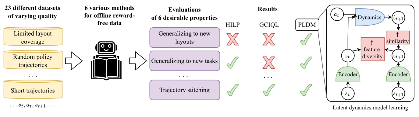
Intuition: a collection of short, imperfect trips may teach how movement works even when it never contains a complete route to the destination. PLDM learns an encoder and action-conditioned latent dynamics, then searches for actions at deployment. This study compares that approach with five reward-free offline learning methods under controlled changes in trajectory length, quality, quantity and maze layout. Planning generalizes particularly well to unseen layouts and a state-avoidance task, but does not win every test: HILP and GCIQL are much stronger when no training trajectory crosses the doorway. The evidence comes from deterministic simulated navigation, including state-based ant control. It does not establish the same ranking for manipulation, partial observability or unrestricted robotics.
1 Introduction
The question is which learning procedure makes best use of reward-free offline trajectories when the eventual task or layout changes. The paper deliberately controls data properties rather than only reporting one favorable benchmark. Its main contribution is a comparative stress test and a simple planning baseline. Generalization claims apply to the tested navigation families and data regimes.
2 Related Work
Goal-conditioned methods learn to reach specified states; zero-shot methods learn reusable skills or representations that can express additional tasks. Optimal-control methods instead search through a learned or known transition model. The paper uses these distinctions to separate what is learned offline from what is optimized when a task is supplied.

3 The Landscape of Available Methods
The comparison includes four goal-conditioned methods, a direction-conditioned zero-shot method and explicit latent-model planning. Each receives offline transitions without recorded rewards.
3.1 Problem Setting
The formal setting assumes deterministic dynamics and fully specified state observations for its model. A task is supplied at evaluation, usually as a goal state. Reward-free data means no reward annotations are provided during collection; goal-conditioned algorithms can still construct their own training objectives from state–goal pairs.
3.2 Reward-free Offline Reinforcement Learning
GCIQL learns a goal-conditioned value and policy, HIQL adds a subgoal hierarchy, CRL learns contrastive state–goal compatibility and GCBC imitates actions conditioned on future goals. HILP learns a distance-like representation plus a policy for moving along latent directions. These are distinct ways to reuse data; Table 1 is a qualitative summary of the following experiments, not an independent benchmark.
| Property (Experiment section) | HILP | HIQL | GCIQL | CRL | GCBC | PLDM |
| Transfer to new environment layouts (4.8) | ★✩✩ | ★✩✩ | ★✩✩ | ★✩✩ | ★✩✩ | ★★★ |
| Transfer to a new task (4.6) | ★★✩ | ★✩✩ | ★✩✩ | ★✩✩ | ★✩✩ | ★★★ |
| Data efficiency (4.3) | ★✩✩ | ★★✩ | ★★★ | ★★✩ | ★★✩ | ★★★ |
| Best-case performance (4.2) | ★★★ | ★★★ | ★★★ | ★★★ | ★★✩ | ★★★ |
| Can learn from random policy trajectories (4.5) | ★★★ | ★✩✩ | ★★★ | ★✩✩ | ★✩✩ | ★★✩ |
| Can stitch suboptimal trajectories (4.4) | ★★★ | ★✩✩ | ★★★ | ★✩✩ | ★✩✩ | ★★✩ |
3.3 Planning with a Latent Dynamics Model
An encoder maps observations to features and an action-conditioned predictor rolls them forward. Training matches predicted features to encoded future observations. Variance and covariance regularization discourage a constant or redundant representation, while an inverse-dynamics objective can require transitions to retain action information. Multiple predictors optionally estimate disagreement. No pixel reconstruction is required.
Equations 1–3
| (1) | ||||
| (2) |
| (3) |
Goal-conditioned planning with PLDM.
At deployment, MPPI samples and reweights candidate actions using latent distance to the goal, plus an optional predictor-disagreement penalty. The latter discourages uncertain plans but is not a calibrated safety guarantee. Replanning incorporates new observations. Changing the planning cost can express a new task without retraining the dynamics. This flexibility costs more inference computation than a single policy call.
Equations 4–7
| (4) | |||
| (5) | |||
| (6) | |||
| (7) |
| Method | Good-quality data | No door-passing trajectories |
| CRL | 189.3 ± 10.7 | 114.7 ± 14.1 |
| GCBC | 186.0 ± 12.0 | 118.4 ± 11.2 |
| GCIQL | 198.0 ± 10.9 | 199.6 ± 10.4 |
| HILP | 100.0 ± 10.0 | 100.0 ± 10.0 |
| HIQL | 196.4 ± 11.3 | 126.3 ± 15.6 |
| PLDM | 197.8 ± 10.7 | 134.4 ± 12.7 |
4 Every Method Can Excel but Few Generalize
The experiments vary one data property at a time where possible, then compare navigation across changed layouts and a higher-dimensional ant controller. The outcome is a map of conditional strengths rather than one universally best method.
4.1 Two-Rooms Environment
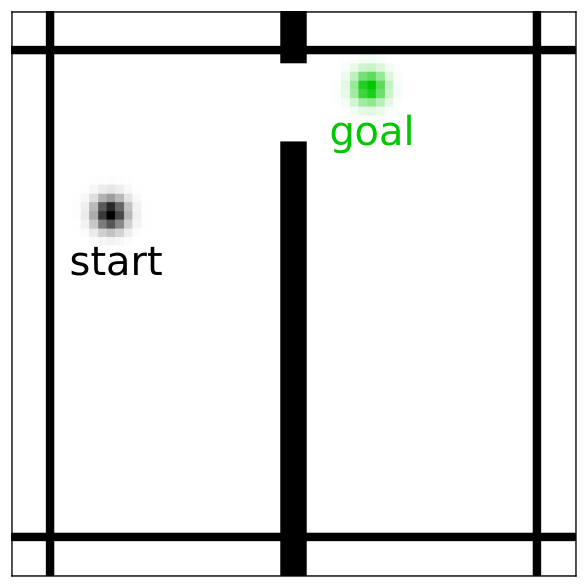
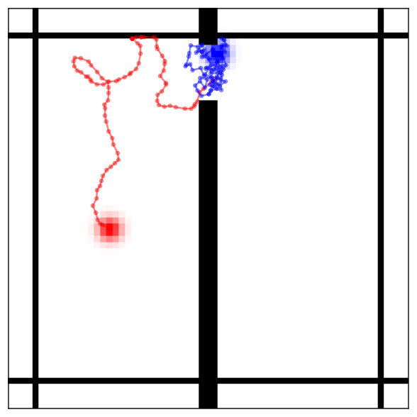
Two-Rooms is a simplified top-down world: actions directly displace a point agent, and the image separates the agent from walls into channels. Persistent random directions generate broad trajectories; independently random directions produce local oscillation. This controlled contrast is useful scientifically but easier than learning real visual locomotion.
4.2 What Methods Excel In-Distribution with a Large High-Quality Dataset?
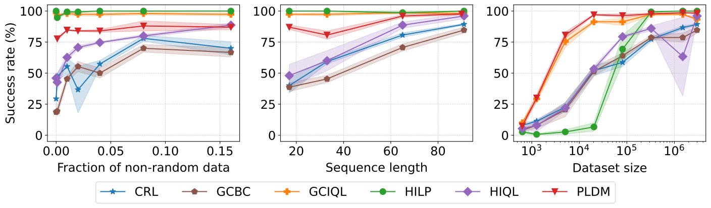
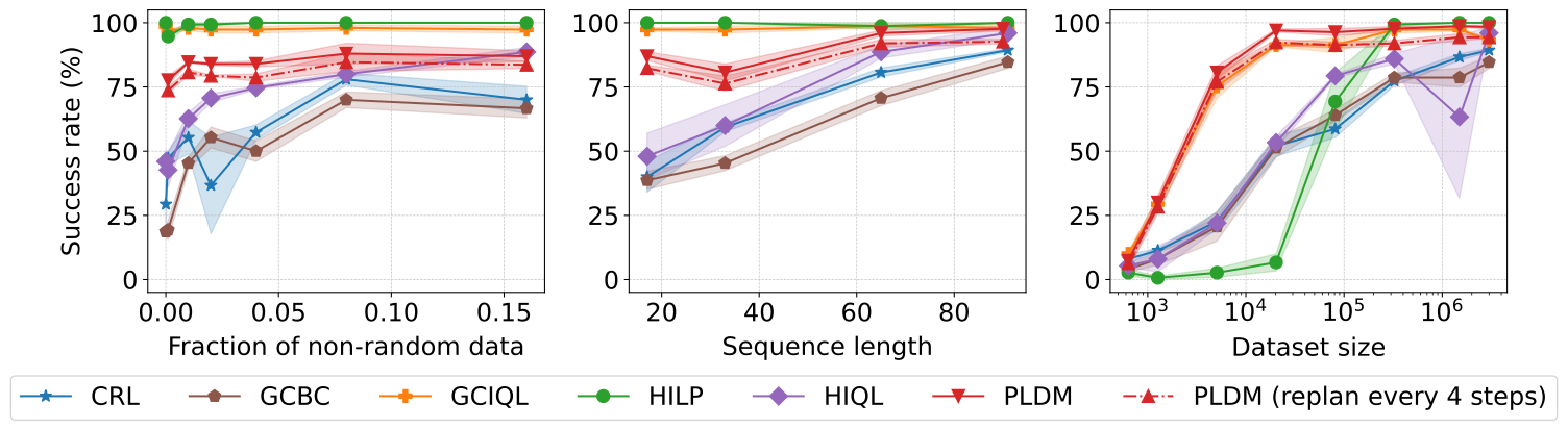
With abundant trajectories that cover the doorway and long routes, every method performs well and several approach perfect success. The harder tests therefore concern coverage, data scarcity and transfer rather than this favorable in-distribution setting alone.
4.3 What Method is the Most Sample-Efficient?
PLDM and GCIQL retain strong performance with relatively few transitions. HILP needs more data in this environment, though it becomes very strong when enough is available. Sample efficiency here measures transitions required for these simulated tasks, not total training or inference cost.
4.4 What Methods Can Stitch Suboptimal Trajectories?
Two stitching tests must be separated. Short episodes can still teach local transitions that a planner composes into a longer route. Removing every doorway-crossing trajectory removes a crucial transition: PLDM drops to 34.4% success, while HILP and GCIQL reach 100%. Learning a model does not automatically reconstruct missing data coverage.
4.5 What Methods Can Learn From Trajectories of a Random Policy?
Independent random actions produce short-range wandering. HILP, GCIQL and PLDM cope better than the other tested goal-conditioned policies. A local transition can still supervise a dynamics model even when its trajectory contains no distant goal. The explanation involving goal-distribution mismatch is plausible, not an isolated causal proof.
4.6 What Methods Can Generalize to a New Task?
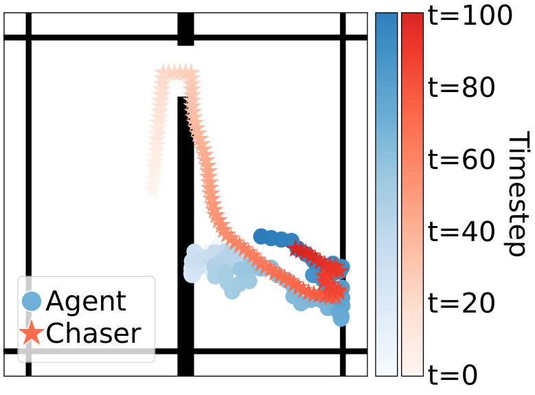
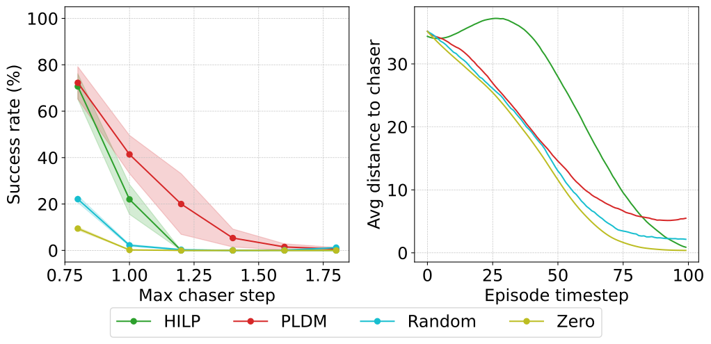
To evade a chaser, PLDM reverses the sign of its goal-distance cost; HILP reverses its skill direction. Neither is retrained. PLDM maintains greater separation in this fixed-dynamics task. This demonstrates one useful cost change, not automatic generalization to any new reward or changed physics.

4.7 Extending to a Higher-Dimensional Control Environment.
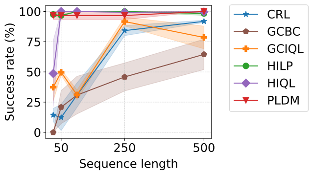
Ant-U-Maze increases control complexity to an eight-dimensional action and 29-dimensional state. The dataset comes from a noisy directional expert policy, rather than raw random joint actions. PLDM, HIQL and HILP stitch short trajectories successfully; GCIQL’s relative advantage from Two-Rooms does not persist. The result is state-based simulation, not camera-only locomotion.
4.8 What Methods Can Generalize to Unseen Environment Layouts?
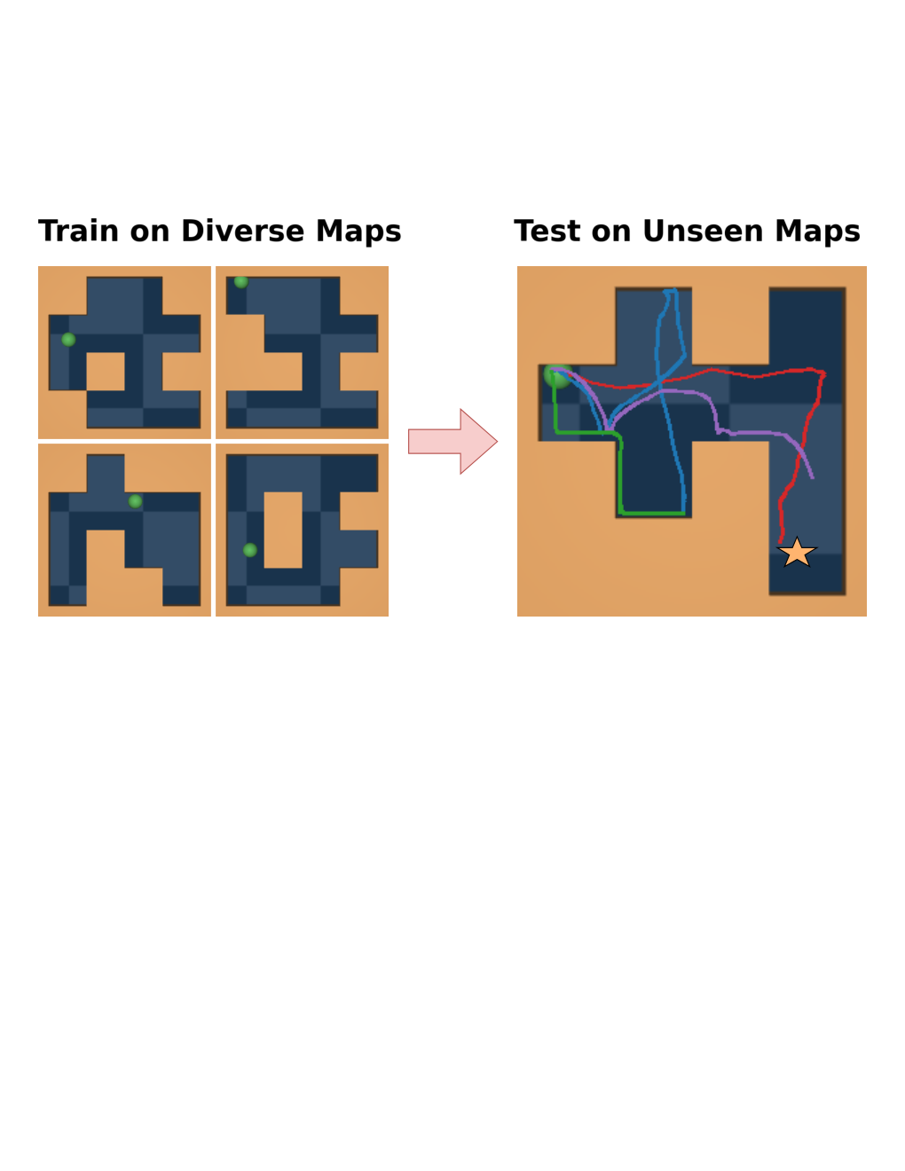
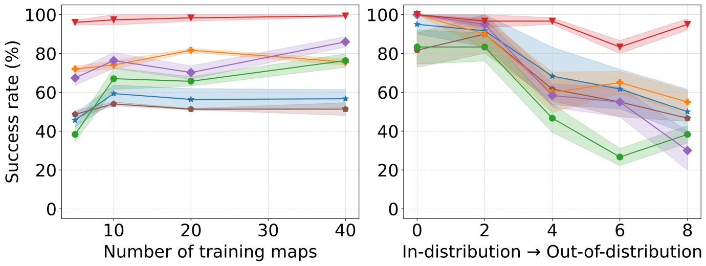
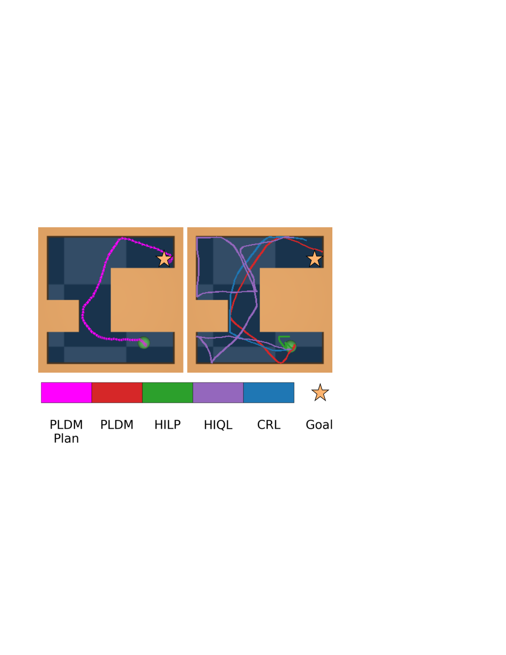
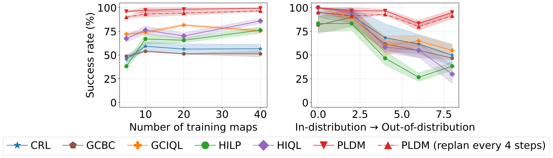
Diverse PointMaze changes obstacle layouts and adds acceleration and velocity. The agent receives a maze image plus velocity. Training layouts are disjoint from test layouts, and edit distance measures the specified layout shift. PLDM transfers much better than the compared policies. Single-layout results show that failure under transfer is different from inability to solve the training task.
5 Conclusion
The practical lesson is to match the method to the data and expected deployment shift. PLDM handles several shifts well; structured skill representations and goal-conditioned value learning can be stronger for missing-transition stitching; plentiful high-quality data makes many policy methods effective. These are empirical guidelines within this suite.
Future work.
The open directions are more complex manipulation, partial observability, accumulated long-rollout errors and reducing planning cost. These are needed before extending the study’s conclusions to general-purpose embodied systems.
Acknowledgments
The source credits computing facilities, grants and institutional support for the study.
Appendix
Table of Contents
Appendix A Reproducibility
Public code includes environments, data generation, training and evaluation. AppendixJ retains the experiment-dependent hyperparameters; reproducing a result requires its corresponding data regime and tuning choices.
Appendix B Visualization of Plans and Trajectories for Diverse PointMaze
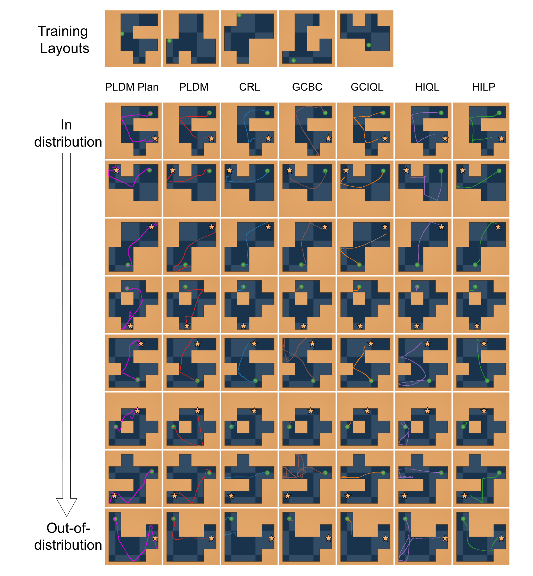
The trajectory panels compare unseen layouts at increasing minimum edit distance from the training set. They make the layout-shift definition concrete and illustrate PLDM’s stronger transfer. Selected successful or failed paths complement the aggregate scores rather than replacing them.
Appendix C Environments and Datasets
C.1 Two-Rooms Environment
The Two-Rooms simulator has no inertia: an action moves the agent immediately, and wall intersection clips that movement. Learning this transition map is substantially simpler than inferring velocities and contacts in realistic control.
C.2 Diverse PointMaze
Diverse PointMaze renders a randomly generated connected four-by-four layout and supplies the agent’s velocity. The dynamics include inertia; actions repeat for four simulator steps. These extra inputs and temporal conventions matter when comparing it with Two-Rooms.
C.2.1 Dataset Generation
Each layout-count condition keeps the total transition count fixed at one million. Increasing training layouts therefore reduces episodes per layout. This tests diversity at a controlled overall data budget, with randomly initialized position and velocity.
| # Transitions | # layouts | # episodes per layout | episode length |
| 1000000 | 5 | 2000 | 100 |
| 1000000 | 10 | 1000 | 100 |
| 1000000 | 20 | 500 | 100 |
| 1000000 | 40 | 250 | 100 |
C.2.2 Evaluation
The same held-out layouts and start–goal trials are used for all agents. One test varies training diversity; another groups test layouts by their minimum grid edit distance to a training layout. That metric measures this particular structural shift, not every possible visual or physical distribution shift.
C.2.3 Results for Single Maze Setting
All methods perform very well on a single fixed maze. The table establishes a useful control: their difficulties on unseen layouts cannot be explained simply by universal inability to navigate.
C.3 Ant U-Maze
The ant benchmark checks trajectory composition with more complex actuation using simulator state observations. It extends control dimensionality without testing visual perception or real-world contact uncertainty.
C.3.1 Dataset Generation
A pretrained directional expert, noisy actions and periodically resampled directions produce five million exploratory transitions. This dataset contains useful locomotion skills even though its downstream goal is not annotated.
C.3.2 Evaluation
The ant starts at one end of a U-shaped room and must reach the diagonally opposite end. Each method is tested on ten trials. This is a specific route requiring a turn, not a broad suite of unfamiliar terrain.
Appendix D Models
Baselines use released OGBench or HILP implementations. Velocity is appended directly for Diverse PointMaze instead of being inferred by stacking images. This aligns the available state information across the compared methods.
D.1 PLDM
D.1.1 Objective for collapse prevention
The anti-collapse loss combines feature spread, low cross-feature covariance, optional temporal smoothness and inverse action reconstruction. The prose describes temporal variance, but the displayed variance formula indexes variance across the batch at each timestep; the original equations are retained, so this distinction should be checked against code before reproduction. Smoothness and action reconstruction trade off persistence against retaining changes.
Equations
D.1.2 Ablations of Objective Components
Removing variance or covariance terms severely harms both tested environments. Removing inverse dynamics hurts Diverse Maze but does not change Two-Rooms in this setting, where its coefficient is already zero. Regularizer importance is therefore conditional on the environment and configured objective.
| Ablation | Success rate (Two-Rooms) | Success rate (Diverse Maze) |
| – | 98.0 ± 1.5 | 98.7 ± 2.8 |
| var coeff () | 13.4 ± 9.2 | 11.4 ± 6.5 |
| cov coeff () | 29.2 ± 4.4 | 7.8 ± 4.1 |
| time sim coeff () | 71.0 ± 3.0 | 95.6 ± 3.2 |
| IDM coeff () | 98.0 ± 1.5 | 75.5 ± 8.2 |
D.1.3 Model Details for Two-Rooms
Two-Rooms uses a small visual encoder and a recurrent predictor whose initial hidden state is the encoded observation. Subsequent action inputs advance that state. Layer normalization is applied to features and predictions. The architecture is small enough for many controlled experiments.
D.1.4 Model Details for Diverse PointMaze Environment
Diverse PointMaze preserves a spatial feature map. Expanded velocity and action planes are concatenated to that map before convolutional prediction. It replans every four interactions and uses a single predictor in the reported hyperparameters. This differs from the recurrent and ensemble configurations elsewhere.
D.1.5 Model Details for Ant-U-Maze
For the ant, an MLP encodes global position and concatenates raw proprioception. A five-model MLP ensemble predicts the next representation. Anti-collapse regularization applies to the learned position features, not raw coordinates that cannot collapse through an encoder.
Appendix E Effects of Uncertainty Regularization via Ensembles
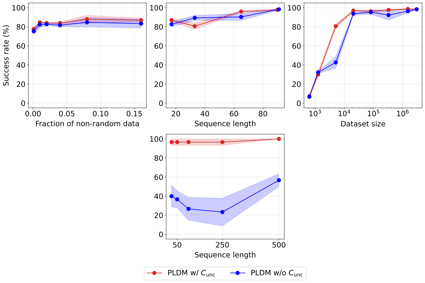
The plots ablate ensemble uncertainty regularization. Its benefit depends on the task and data regime, so disagreement should be treated as a configurable empirical aid. The method also has a single-predictor configuration and is not inherently dependent on an ensemble.
Appendix F Analyzing planning time of PLDM
Replanning every step is slower than policy execution. In Two-Rooms, replanning every four steps reduces average episode time from 16.0 to 4.8 seconds while retaining 95% of the every-step success rate; every 32 steps retains only 62%. Less frequent feedback creates a clear speed–reliability tradeoff.
| Method | Replan Every | Time per episode (seconds) | Normalized Success Rate |
| PLDM | 1 | 16.0 ± 0.13 | 1.00 |
| PLDM | 4 | 4.8 ± 0.09 | 0.95 |
| PLDM | 16 | 2.6 ± 0.07 | 0.90 |
| PLDM | 32 | 2.2 ± 0.07 | 0.62 |
| GCIQL | – | 3.6 ± 0.10 | – |
| HIQL | – | 4.0 ± 0.08 | – |
F.1 Evaluating PLDM Performance With Adjusted Inference Compute Budget
Additional plots compare the reduced-frequency planner under a more similar inference budget. Much of its performance remains, though some is lost. Matching total runtime does not make the internal computation or action-feedback frequency identical.
Appendix G Extended Baselines: Input Reconstruction Learning and TD-MPC2
These controls replace the representation objective or adapt existing world models to the reward-free task. They test particular configurations and should be interpreted with the adaptations in view.
Dreamer
DreamerV3 loses reward training and learned policy execution, then uses latent-distance planning. The authors explicitly acknowledge that this differs from its intended design. Poor performance here is evidence about this reward-free adaptation, not the full Dreamer system.
Reconstruction
A closer reconstruction control retains PLDM’s encoder and predictor architecture while replacing its regularization with pixel reconstruction. It isolates that objective change more directly than comparing entirely different model families.
TD-MPC2
Reward removal causes TD-MPC2 to collapse in this setup. Adding inverse dynamics helps but remains weak; that modified variant has only one tested seed. The table supports the need to prevent collapse under this altered objective, not a general comparison against normally trained TD-MPC2.
| Method | Success rate |
| CRL | 189.3 ± 11.2 |
| GCBC | 186.0 ± 14.5 |
| GCIQL | 198.0 ± 10.9 |
| HILP | 100.0 ± 10.0 |
| HIQL | 196.4 ± 13.0 |
| PLDM | 197.4 ± 11.3 |
| DreamerV3 | 124.0 ± 16.9 |
| Reconstruction | 126.2 ± 13.9 |
| TD-MPC2 | 110.0 ± 10.0 |
| TD-MPC2 + IDM | 135.0 ± 10.0 |
Appendix H Analyzing Statistical Significance of Results
Welch tests compare methods using pooled settings and selected ten-seed runs. Several comparisons with HILP and GCIQL are not significant, consistent with their competitive performance. Pooling different data conditions provides one aggregate analysis and should not be read as proving superiority in each individual condition.
| Sequence length |
|
Dataset size |
|
| |||||||
| CRL | ✓(p=1.68e-03) | ✓(p=8.46e-07) | ✓(p=1.13e-02) | ✓(p=3.43e-10) | ✓(p=4.02e-03) | ||||||
| GCBC | ✓(p=4.25e-04) | ✓(p=1.46e-08) | ✓(p=7.26e-03) | ✓(p=3.71e-20) | ✓(p=1.94e-05) | ||||||
| GCIQL | ✗ | ✗ | ✗ | ✓(p=1.29e-12) | ✓(p=1.22e-03) | ||||||
| HILP | ✗ | ✗ | ✓(p=2.11e-02) | ✓(p=6.54e-06) | ✓(p=4.10e-05) | ||||||
| HIQL | ✓(p=2.21e-02) | ✓(p=9.26e-05) | ✓(p=2.39e-02) | ✓(p=2.84e-06) | ✓(p=9.01e-03) |
| Sequence length 17 |
|
Dataset size 20312 | |||
| CRL | ✓(p=3.82e-11) | ✓(p=1.13e-07) | ✓(p=6.76e-11) | ||
| GCBC | ✓(p=1.54e-12) | ✓(p=5.75e-10) | ✓(p=1.88e-14) | ||
| GCIQL | ✗ | ✗ | ✗ | ||
| HILP | ✗ | ✗ | ✓(p=2.49e-19) | ||
| HIQL | ✓(p=8.89e-05) | ✓(p=2.83e-07) | ✓(p=2.65e-11) |
Appendix I Analyzing HILP’s Out-of-Distribution Generalization
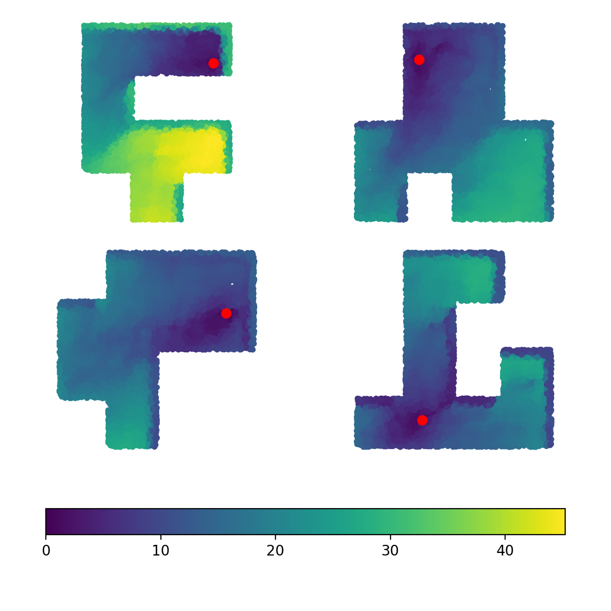
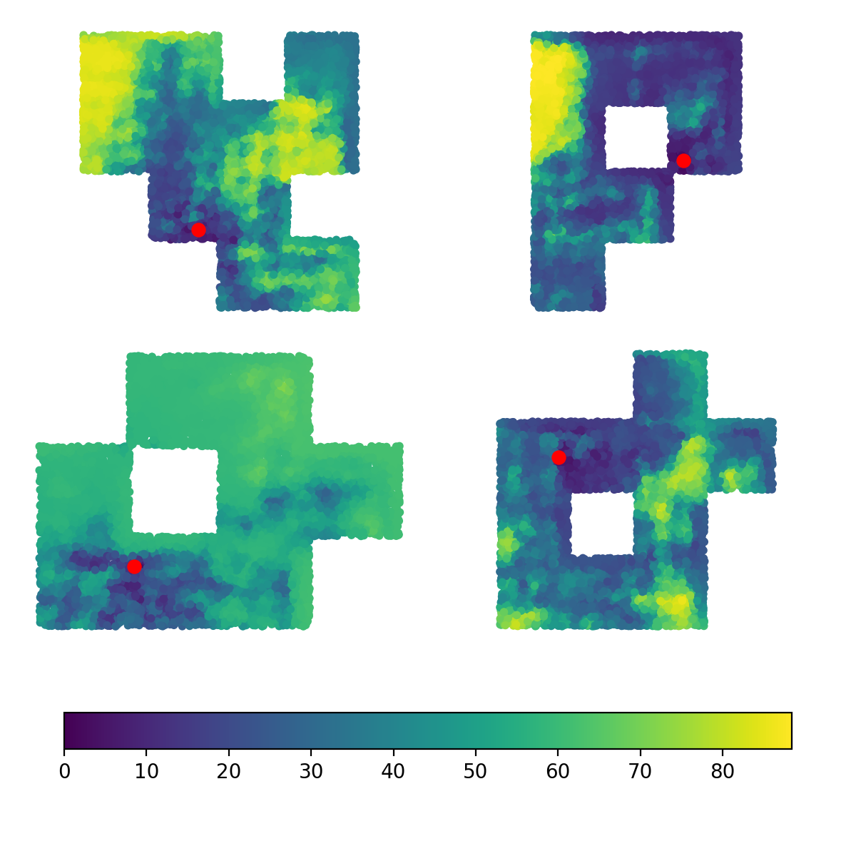
Visualized HILP distances align with routes on training layouts but become noisy on held-out layouts. This supports representation transfer as a failure mode in the examined models. It is a diagnostic example rather than proof that the representation must always fail under layout changes.
Appendix J Hyperparameters
J.1 CRL, GCBC, GCIQL, HIQL, HILP
Baseline defaults come from released repositories, with the reported task-specific adjustments. Equivalent architectures do not imply identical optimal learning rates or goal-sampling distributions.
J.1.1 Two-Rooms
Grid searches cover good-quality and short-trajectory conditions, then selected settings are applied across tests. Different regimes receive some different parameters; the comparison is not one universal untuned configuration.
HILP.
HILP uses a fixed learning rate and expectiles in these Two-Rooms experiments.
GCIQL.
GCIQL changes behavior-cloning weight and random-goal sampling for particular data regimes. These settings influence conservative policy learning and the goals seen during training.
HIQL.
HIQL changes learning rate and random-goal probability in the short-trajectory conditions while retaining its two-level policy design.
J.1.2 Diverse PointMaze
The retained tables give learning rates, expectiles and goal-sampling parameters for each layout-count condition. Reproduction should use the row matching the tested training diversity.
| Dataset | CRL | GCBC | HILP | |
| LR | LR | LR | Expectile | |
| 5 layouts | 0.0003 | 0.0003 | 0.0001 | 0.9 |
| 10 layouts | 0.0003 | 0.0001 | 0.0001 | 0.9 |
| 20 layouts | 0.0003 | 0.0001 | 0.0001 | 0.9 |
| 40 layouts | 0.0003 | 0.0001 | 0.0001 | 0.9 |
| Dataset | GCIQL | HIQL | |||||||||||||
| LR | Expectile |
|
|
LR | Expectile |
|
| ||||||||
| 5 layouts | 0.0003 | 0.6 | 0.3 | 0.15 | 0.00003 | 0.6 | 1.0 | 0.6 | |||||||
| 10 layouts | 0.0003 | 0.6 | 0.3 | 0.15 | 0.0001 | 0.7 | 3.0 | 0.0 | |||||||
| 20 layouts | 0.0003 | 0.6 | 0.3 | 0.15 | 0.00003 | 0.6 | 1.0 | 0.6 | |||||||
| 40 layouts | 0.0003 | 0.6 | 0.3 | 0.15 | 0.0001 | 0.7 | 3.0 | 0.0 | |||||||
J.1.3 Ant U-Maze
Ant settings vary with episode length and method. The tables retain those tuning choices rather than suggesting that every method used one shared hyperparameter set.
| Seq Len | CRL | GCBC | HILP | ||||||||
| LR |
|
|
LR | LR |
| ||||||
| 25 | 3e-5 | 0.1 | 0.3 | 3e-3 | 3e-4 | 0.6 / 0.8 | |||||
| 50 | 3e-5 | 0.1 | 0.3 | 3e-3 | 3e-4 | 0.6 / 0.8 | |||||
| 100 | 3e-4 | 0.1 | 0.0 | 3e-3 | 3e-4 | 0.6 / 0.8 | |||||
| 250 | 3e-4 | 0.1 | 0.0 | 3e-3 | 3e-4 | 0.6 / 0.8 | |||||
| 500 | 3e-4 | 0.1 | 0.0 | 3e-3 | 3e-4 | 0.6 / 0.8 | |||||
| Seq Len | GCIQL | HIQL | |||||||||||||
| LR | Expectile |
|
|
LR | Expectile |
|
| ||||||||
| 25 | 3e-5 | 0.9 | 0.15 | 0.15 | 3e-4 | 0.6 | 3.0 | 0.6 | |||||||
| 50 | 3e-5 | 0.9 | 0.15 | 0.15 | 3e-4 | 0.6 | 3.0 | 0.6 | |||||||
| 100 | 3e-5 | 0.9 | 0.15 | 0.15 | 3e-4 | 0.6 | 3.0 | 0.6 | |||||||
| 250 | 3e-4 | 0.9 | 0.3 | 0.0 | 3e-4 | 0.6 | 3.0 | 0.6 | |||||||
| 500 | 3e-4 | 0.9 | 0.3 | 0.0 | 3e-4 | 0.6 | 3.0 | 0.6 | |||||||
J.2 PLDM
J.2.1 Two-Rooms
Two-Rooms uses a five-predictor ensemble and a horizon of 16 model steps, but the regularization weights and learning rate vary by dataset. Inverse dynamics is disabled in this configuration. The table repeats one non-random-data row; the printed record is retained.
| Hyperparameter | Value |
| Batch Size | 64 |
| Predictor Horizon () | 16 |
| Optimizer | Adam |
| Scheduler | Cosine |
| Ensemble size | 5 |
| 0 | |
| MPPI noise | 5 |
| MPPI samples | 500 |
| MPPI | 0.005 |
| Planner coeff | 0.0001 |
| Planner coeff | 0.9 |
| Dataset | LR | |||
| Sequence length = 91 | 0.0007 | 4.0 | 6.9 | 0.75 |
| Sequence length = 65 | 0.0003 | 5.0 | 6.9 | 0.75 |
| Sequence length = 33 | 0.0014 | 3.5 | 6.9 | 0.75 |
| Sequence length = 17 | 0.0028 | 3.0 | 6.9 | 0.75 |
| Dataset size = 634 | 0.0030 | 2.2 | 13.0 | 0.50 |
| Dataset size = 1269 | 0.0010 | 2.2 | 13.0 | 0.50 |
| Dataset size = 5078 | 0.0005 | 2.2 | 13.0 | 0.90 |
| Dataset size = 20312 | 0.0030 | 2.2 | 13.0 | 0.50 |
| Dataset size = 81250 | 0.0010 | 2.2 | 13.0 | 0.50 |
| Dataset size = 325k | 0.0010 | 4.0 | 6.9 | 0.75 |
| Dataset size = 1500k | 0.0010 | 4.0 | 6.9 | 0.75 |
| Non-random % = 0.001 | 0.0007 | 3.9 | 6.9 | 0.74 |
| Non-random % = 0.01 | 0.0007 | 3.9 | 6.5 | 0.19 |
| Non-random % = 0.02 | 0.0007 | 3.9 | 6.5 | 0.72 |
| Non-random % = 0.04 | 0.0007 | 3.9 | 6.5 | 0.65 |
| Non-random % = 0.08 | 0.0007 | 3.9 | 6.5 | 0.24 |
| Non-random % = 0.08 | 0.0007 | 3.9 | 6.5 | 0.24 |
| Wall crossing % = 0 | 0.0007 | 4.0 | 6.9 | 0.75 |
J.2.2 Diverse PointMaze
Diverse PointMaze trains for five epochs with one predictor. The source repeats the five-layout row and omits an explicitly labeled ten-layout row in its dataset-specific table. The edition preserves that ambiguity rather than inventing missing settings.
| Hyperparameter | Value |
| Epochs | 5 |
| Batch Size | 128 |
| Predictor Horizon () | 16 |
| Optimizer | Adam |
| Scheduler | Cosine |
| Ensemble size | 1 |
| MPPI noise | 5 |
| MPPI samples | 500 |
| MPPI | 0.0025 |
| Dataset | LR | ||||
| # map layouts = 5 | 0.04 | 35.0 | 12.0 | 0.1 | 5.4 |
| # map layouts = 5 | 0.04 | 35.0 | 12.0 | 0.1 | 5.4 |
| # map layouts = 20 | 0.05 | 54.5 | 15.5 | 0.1 | 5.2 |
| # map layouts = 40 | 0.05 | 54.5 | 15.5 | 0.1 | 5.2 |
J.2.3 Ant-U-Maze
Ant uses a five-predictor ensemble and retains inverse dynamics, with learning rate changing by trajectory length. These settings differ materially from the simpler image-navigation configurations.
| Dataset | LR |
| Sequence length = 25 | 0.006 |
| Sequence length = 50 | 0.004 |
| Sequence length = 100 | 0.003 |
| Sequence length = 250 | 0.001 |
| Sequence length = 500 | 0.001 |
J.3 Further related work
Further related work connects conservative offline learning, large robot datasets and self-supervised representations. These links motivate the study without enlarging its tested task scope.
Appendix K Discussion of Computational Costs
A run uses one GPU and up to a day on a V100, while the complete research process is estimated at 500–2000 GPU-days. Per-run affordability and aggregate experimental cost are different quantities.
Appendix L Limitations
The principal limits are navigation-only experiments, deterministic/fully observed settings and increased planning cost. The compute-matched tests partly address latency, but manipulation, partial observability and broad real-world transfer remain untested.