Overview
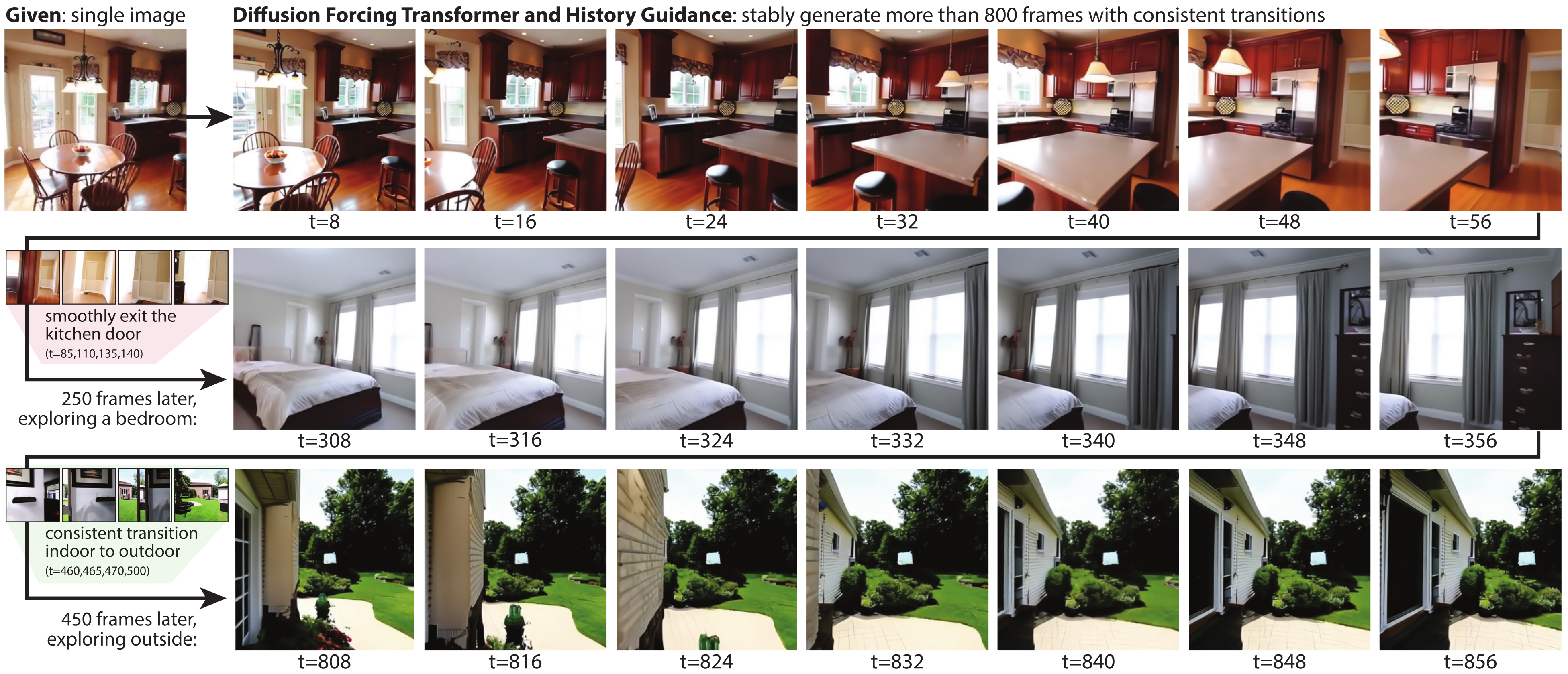
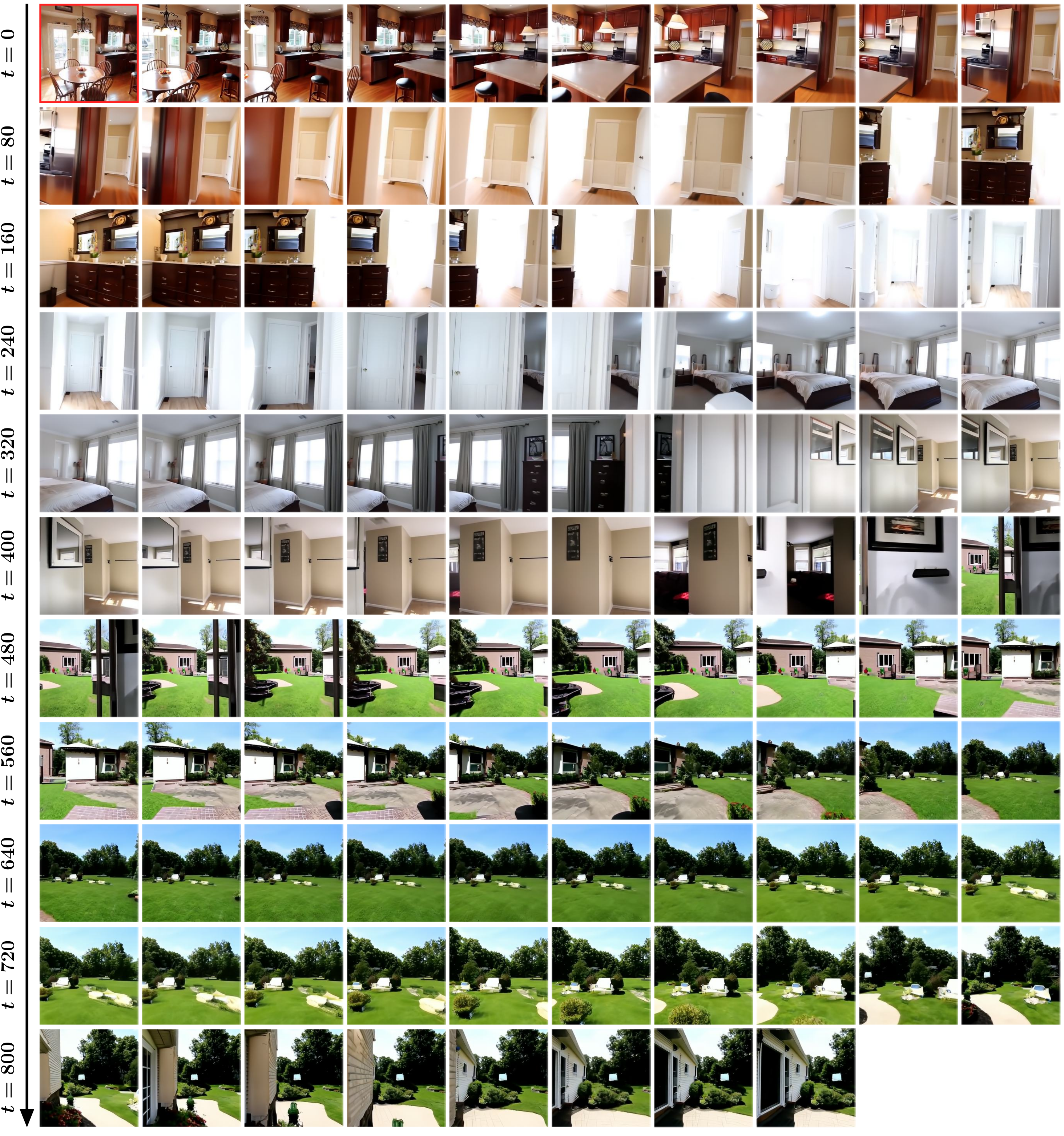
The opening example shows frames from an 862-frame navigation video. A single test-set image initializes generation; the full showcase also uses user-directed camera poses, coarse rollout, interpolation, and stabilization, as detailed in the supplement.
At a glance
The Diffusion Forcing Transformer (DFoT) trains a video denoiser with an independently sampled noise level for each frame. Clean frames act as history, fully noised frames hide history, and partially noised frames provide intermediate conditioning. This supports arbitrary subsets of observed frames without a separate fixed-size history input.
History Guidance combines scores from complete, shortened, or partially masked histories. It improves quality and consistency in the tested video models, and can trade those gains against motion and diversity. Temporal composition also helps on unusual camera histories, Minecraft rollouts, and a fruit-swapping robot task. The long navigation showcases combine user-directed camera poses, coarse rollout, interpolation, and stabilization.
1 Introduction
Classifier-free guidance usually strengthens a text or image condition by comparing conditional and unconditional scores. This work treats video history itself as a controllable condition: which frames are visible, how many are retained, and how strongly each is corrupted.
Building on Diffusion Forcing, DFoT extends independent frame noise to non-causal Transformers. Vanilla guidance uses one history; temporal guidance combines several windows; fractional guidance uses partially noised history. Their composition provides a flexible sampling interface, while experiments test the benefits and the limits of these choices.
2 Preliminaries and Related Work
A diffusion model learns to reverse a noising process, often through a noise- or velocity-prediction parameterization. Conditional sampling uses the resulting score; classifier-free guidance extrapolates from an unconditional score toward a conditional one. Larger guidance weights can improve condition adherence while reducing diversity.
Video models often condition on a fixed first image or small frame set. DFoT instead places history and generated frames in one sequence, extending the per-frame noising idea of Diffusion Forcing to state-free, non-causal architectures such as DiT and U-ViT. Composition of several conditional scores motivates guidance beyond a single CFG difference.
Equation 1
| (1) |
3 Challenges when Guiding with History
Let H index observed history and G index frames to generate. Both are subsets of the same video, so generated frames can later become history. Supporting arbitrary H requires conditional and unconditional estimates for variable subsets, rather than a separate fixed-size conditioning vector.
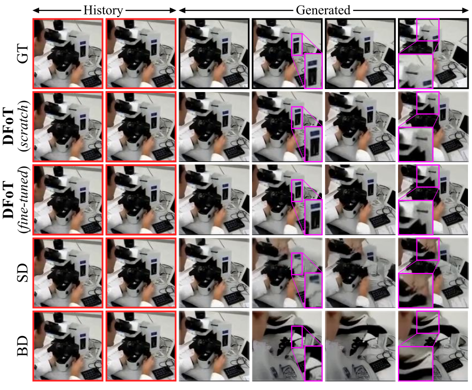
A direct alternative is to randomly drop whole history frames during training. The binary-dropout ablation supports flexible conditioning but performs worse in the matched experiments. The proposed explanation is reduced use of tokens for the prediction loss; this is an empirical hypothesis, not a proof that binary dropout must always underperform.
Equation 2
| (2) |
4 The Diffusion Forcing Transformer
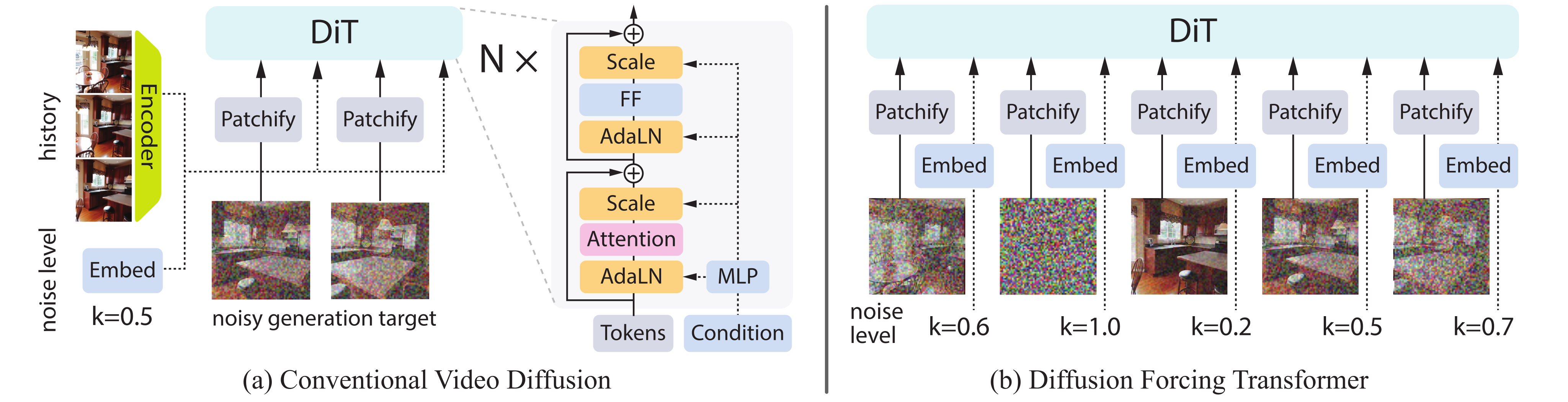
DFoT interprets noising as masking. During training, each frame receives an independent noise level and contributes to the denoising objective. During sampling, observed frames are clean, generated frames follow the sampler’s noise schedule, and excluded history is replaced by noise. This makes interpolation, extrapolation, and mixed observed subsets available to the same trained model.
The architecture must accept frame-specific noise embeddings; compatible full-sequence Transformers can be fine-tuned rather than retrained from scratch. The appendix motivates the objective with path-wise variational bounds, but explicitly leaves cross-path consistency unresolved. Its printed ELBO formulas also contain sign and indexing problems, discussed below; the empirical results do not depend on accepting those formulas as a complete proof.
Equations 3–4
| (3) |
| (4) |
Theorem 4.1 (Informal).
The DFoT training objective (Equation 4) optimizes a reweighting of an Evidence Lower Bound (ELBO) on the expected log-likelihoods.
| Flexible? | Method | FVD | |
| Industry size and compute | ✗ | MAGVIT-v2 (Yu et al., 2023b) | 4.30.1 |
| W.A.L.T (Gupta et al., 2024) | 3.30.1 | ||
| Rolling Diffusion (Ruhe et al., 2024) | 5.2 | ||
| ▲ | Video Diffusion (Ho et al., 2022b) | 16.20.3 | |
| ✔ | MAGVIT (Yu et al., 2023a) | 9.90.3 | |
| Same Architecture | ✗ | SD | 4.80.0 |
| ▲ | FS | 95.50.4 | |
| ✔ | BD | 6.40.1 | |
| DFoT (scratch) | 4.30.1 | ||
| DFoT (fine-tuned from FS) | 4.70.0 |
5 History Guidance
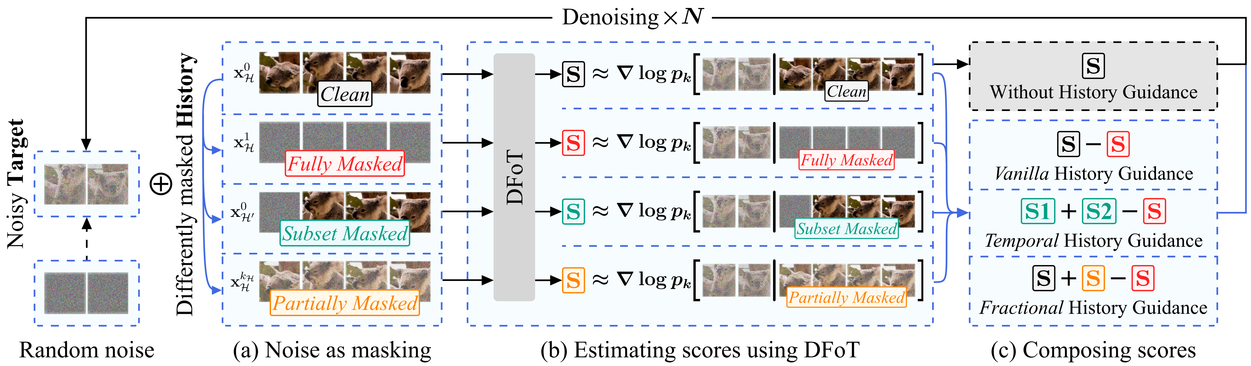
Vanilla History Guidance (HG-v) applies CFG using a chosen clean history. The unconditional branch replaces that history with full noise. Temporal guidance (HG-t) combines scores from different history windows, aiming to retain useful long-range information while reducing sensitivity to unusual long contexts.
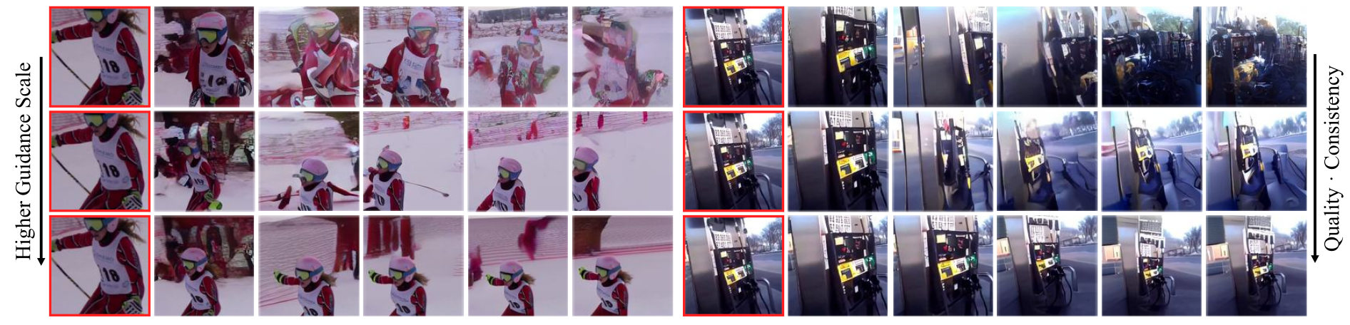
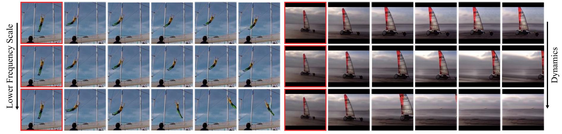
Fractional guidance (HG-f) adds a score difference based on partially noised history. This weakens constraints from less reliable signal components and reduces the tendency of strong vanilla guidance to copy a recent frame. Gaussian noise does not intrinsically remove only high frequencies: the low-pass interpretation depends on the signal’s spectral power and is justified only in a simplified model.
The general formula combines histories with different lengths and noise levels. It is a flexible sampling heuristic, not a guarantee that arbitrary weighted scores equal the true full-history conditional distribution. The retained equations distinguish ordinary conditioning, CFG, temporal composition, and fractional guidance.
The fractional-guidance coefficient is written differently in Equation 6 and the sampler’s example: one uses ω, the other ω−1 for the partially masked score difference. Both source expressions are retained; the appendix example is the one that reduces to ordinary conditioning at weight one.
Equation 5
| (5) |

Equation 6
| (6) |
6 Experiments
Experiments first compare unguided base models, then test guidance, unusual histories, long contexts, robotic control, and extended navigation videos. Separate models are trained for each dataset.
6.1 Experimental Setup
Kinetics-600 supplies the standard 128×128 prediction benchmark. RealEstate10K uses 256×256 images and camera poses; Minecraft uses action-conditioned navigation; Fruit Swapping tests memory and reactivity in a physical robot.
Matched baselines are standard fixed-history diffusion (SD), binary-dropout diffusion (BD), and unconditional full-sequence diffusion with reconstruction guidance (FS). FVD measures video-feature distribution discrepancy, VBench separates quality/consistency/dynamics, and LPIPS compares generated frames with ground truth on constrained tasks. These metrics answer different questions and are not interchangeable.
6.2 Evaluating the Diffusion Forcing Transformer
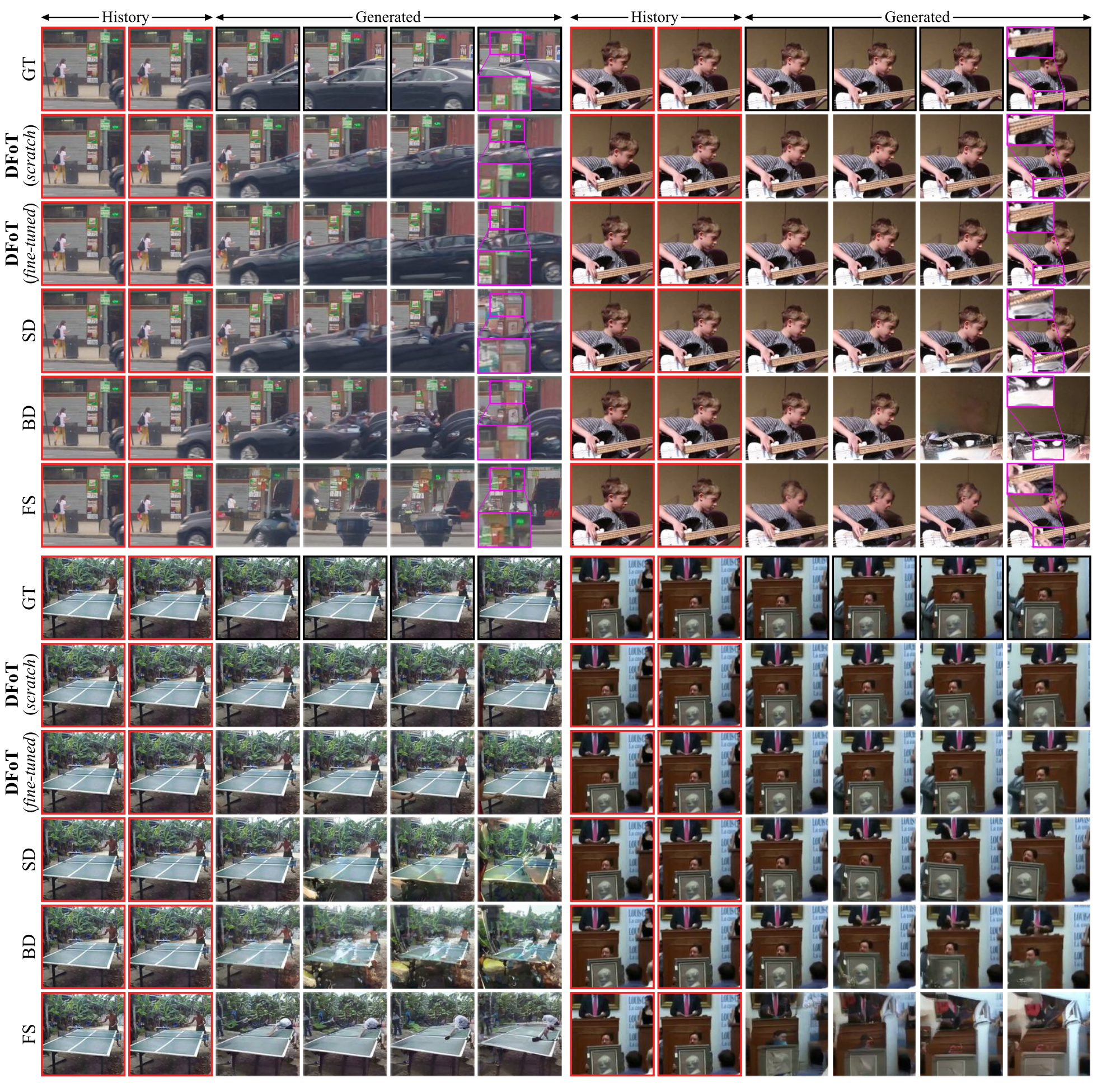
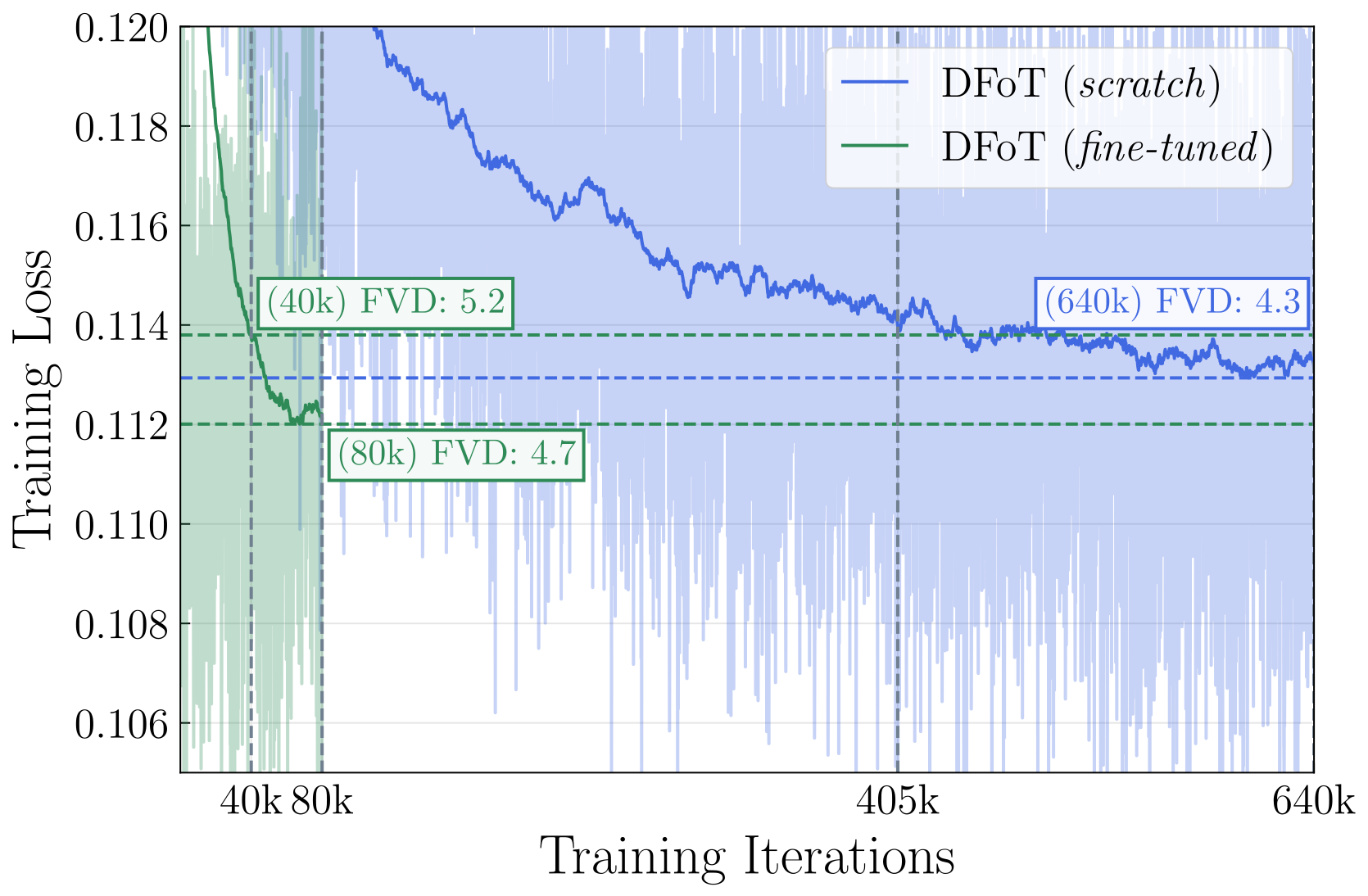
On five-frame-to-eleven-frame Kinetics prediction, unguided DFoT reaches FVD 4.3±0.1, compared with SD 4.8±0.0, BD 6.4±0.1, and FS 95.5±0.4 under the matched pipeline. Fine-tuning FS for 80,000 additional steps reaches 4.7±0.0. These extra steps are 12.5% of the 640,000-step scratch run, excluding the pretrained model’s cost.
Published literature models use different resources and architectures: W.A.L.T. scores 3.3±0.1 and MAGVIT-v2 4.3±0.1. Thus DFoT leads the matched generic baselines, ties the reported MAGVIT-v2 mean, and trails W.A.L.T. Flexible interpolation and mixed-history examples provide qualitative evidence for the shared conditioning interface.
6.3 Improving Video Generation via History Guidance
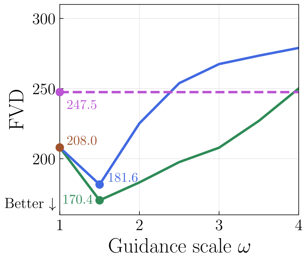
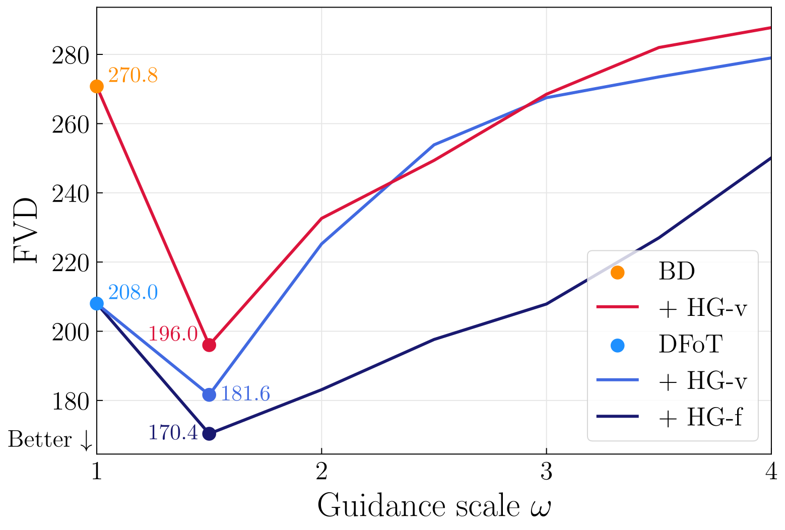
The rollout experiment generates 59 frames after five observed frames and evaluates 1,024 total 64-frame videos. Moderate vanilla guidance improves FVD from 208.0 to 181.6 at weight 1.5, while fractional guidance reaches 170.4. SD scores 247.5 and FS 1040 in this longer setting; these values should not be compared directly with the short-video benchmark.
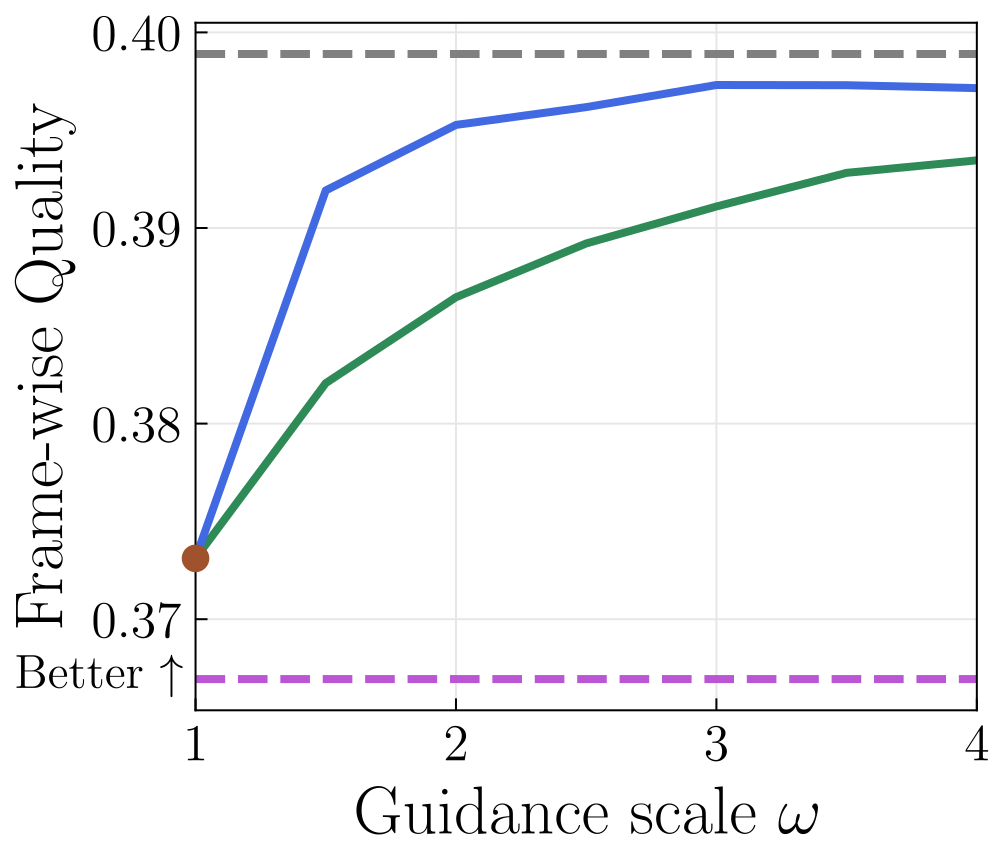
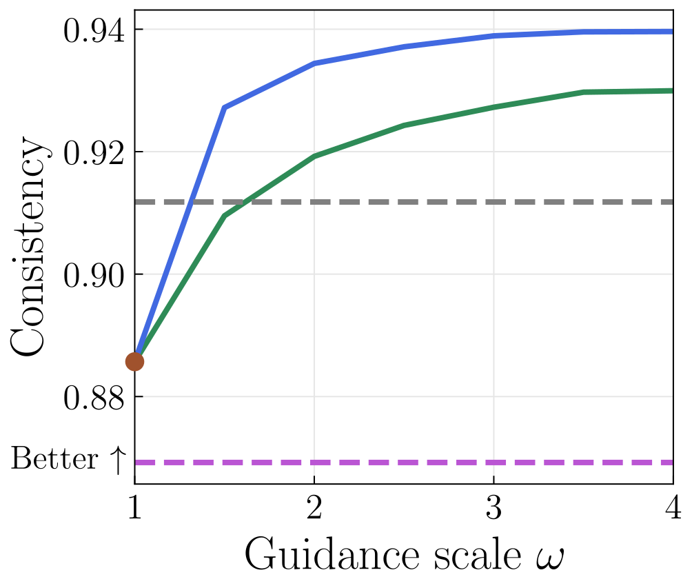
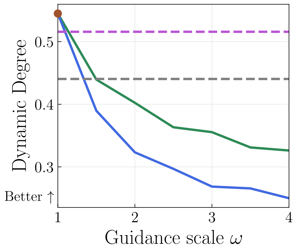
Increasing vanilla guidance improves frame quality and consistency but eventually makes videos static and worsens FVD. Fractional masking restores some dynamics while keeping much of the quality gain. The selected masking level and guidance scale are experimental choices, not universal optima.
6.4 New Abilities via Temporal History Guidance
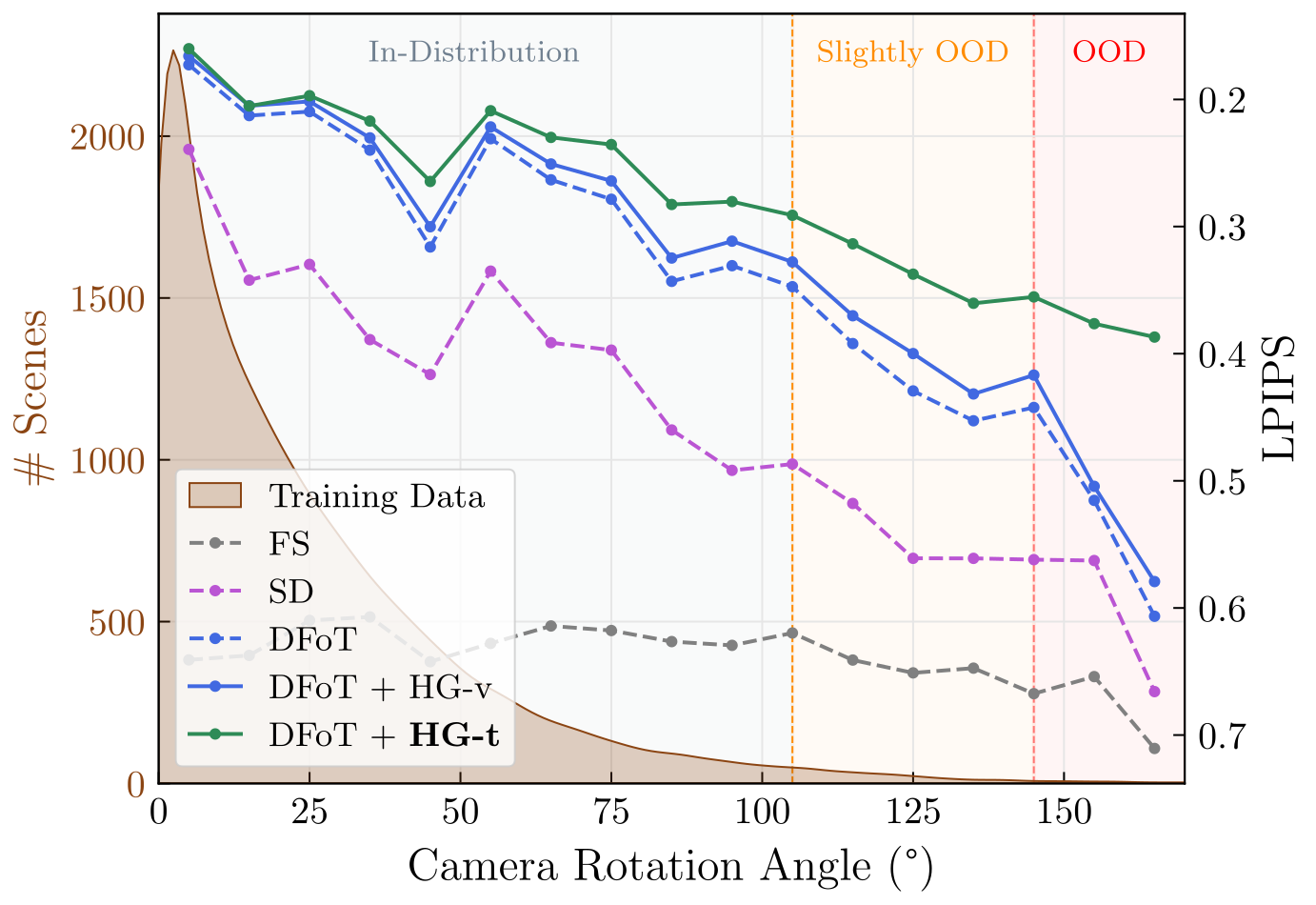
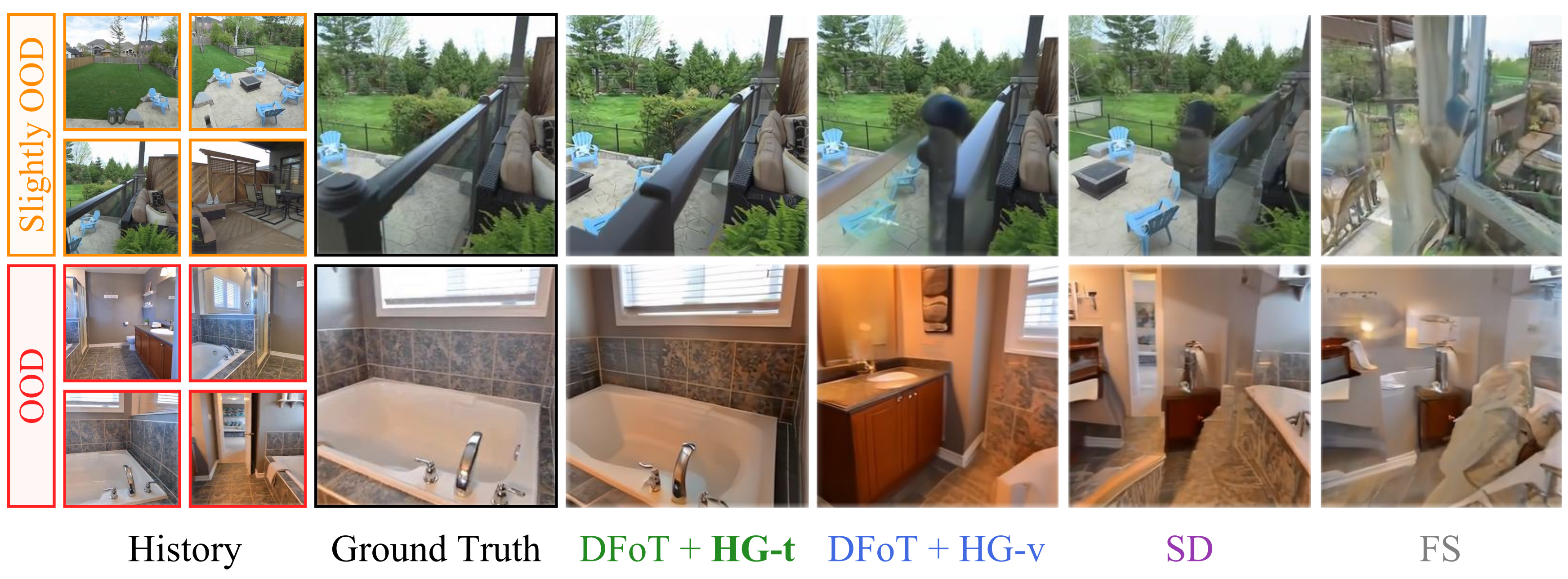
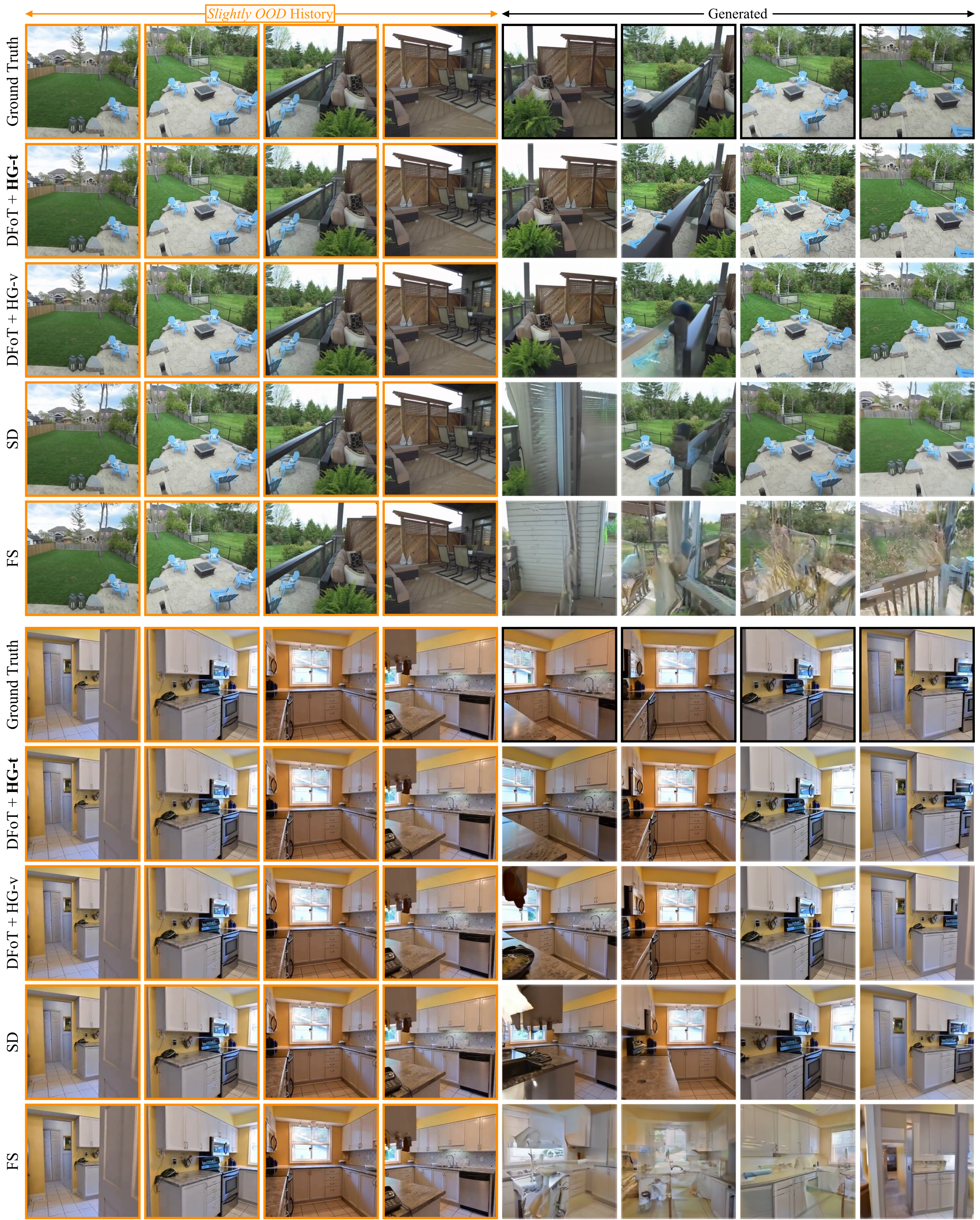
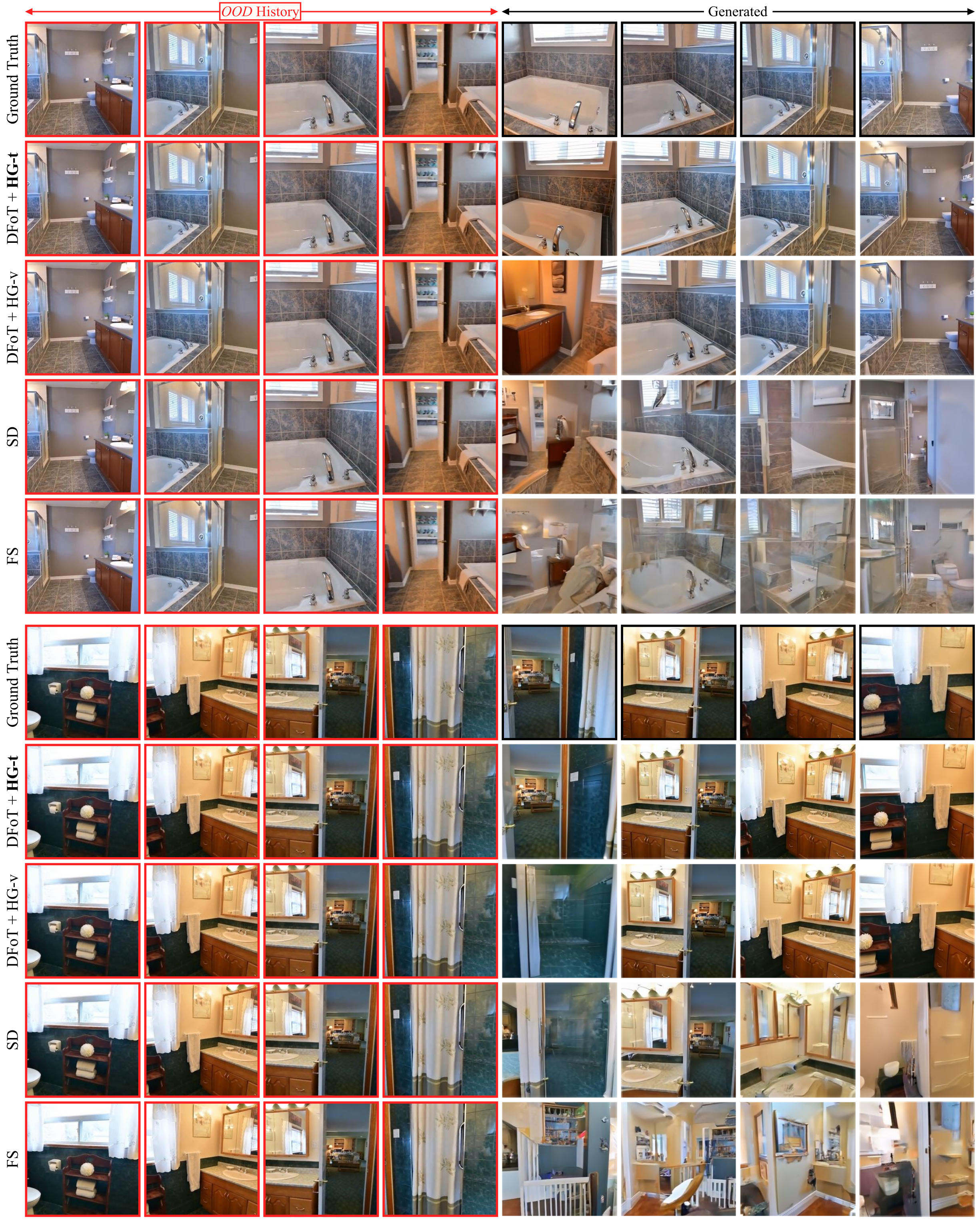
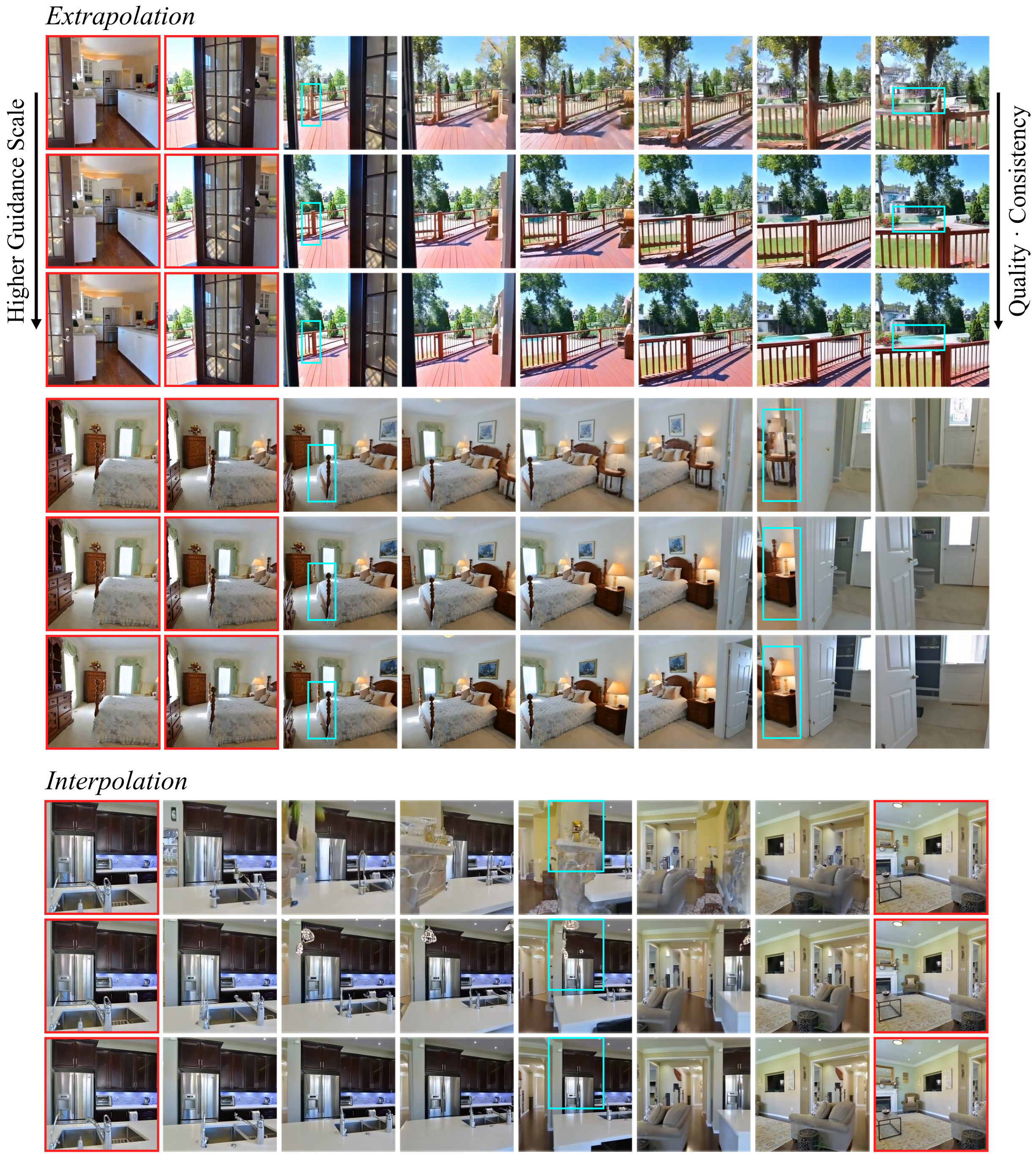
On RealEstate10K, histories spanning unusually large camera rotations cause large errors for the baselines. Composing overlapping shorter histories, and in this experiment shorter generation subsets, improves interpolation LPIPS across the sparsely represented rotation ranges.
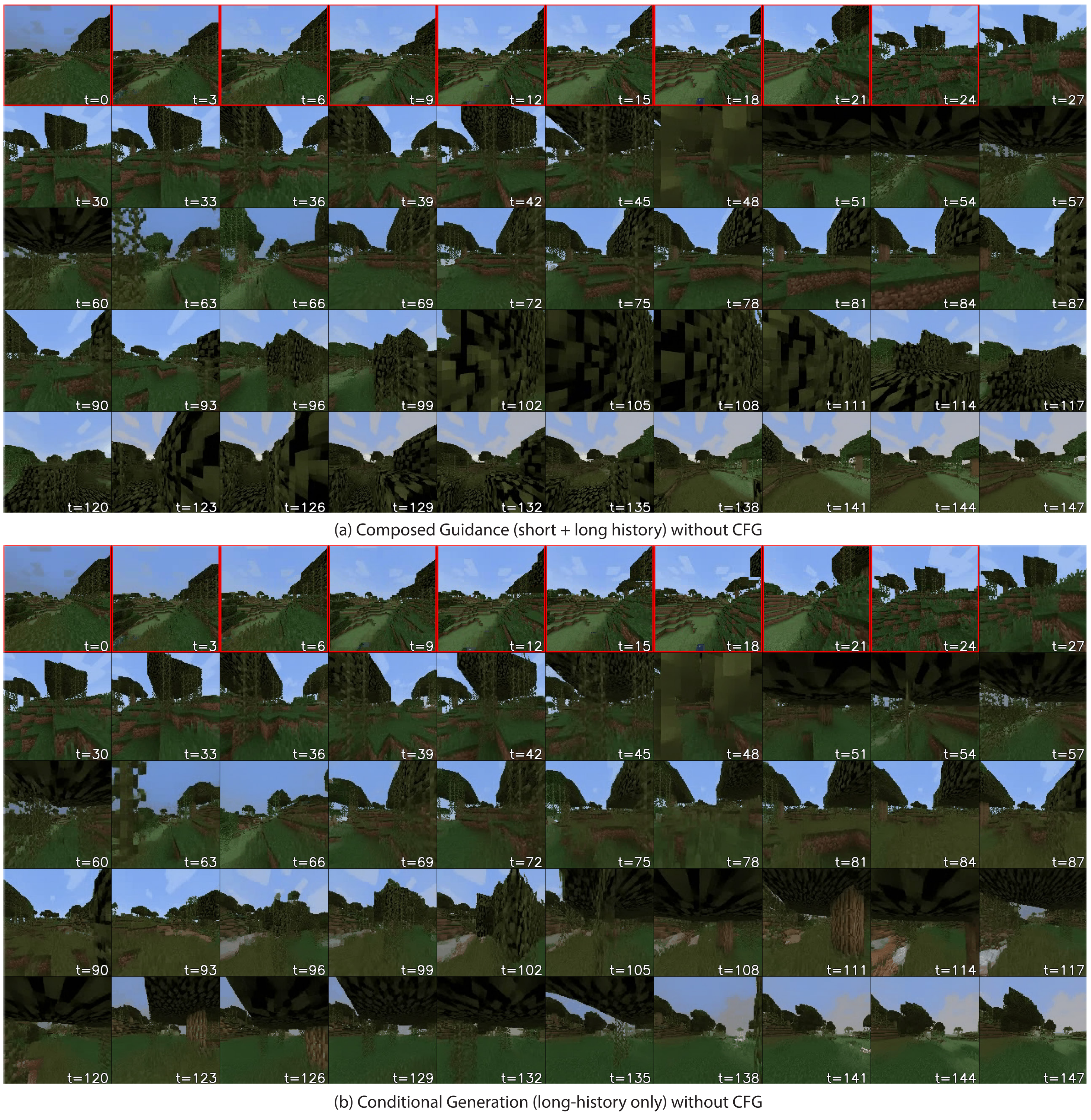
For action-conditioned Minecraft, equal-weight short- and long-context scores reduce FVD from 97.625 to 79.19 over 125 generated frames. In Fruit Swapping, composed histories achieve 83% success under the main human-perturbation protocol, with 100 randomized setups. Stronger perturbations reduce the reported success to 28%. These experiments support complementary memory and reactive behavior on the tested tasks, rather than proving that other models cannot solve them.
6.5 Ultra Long Video Generation
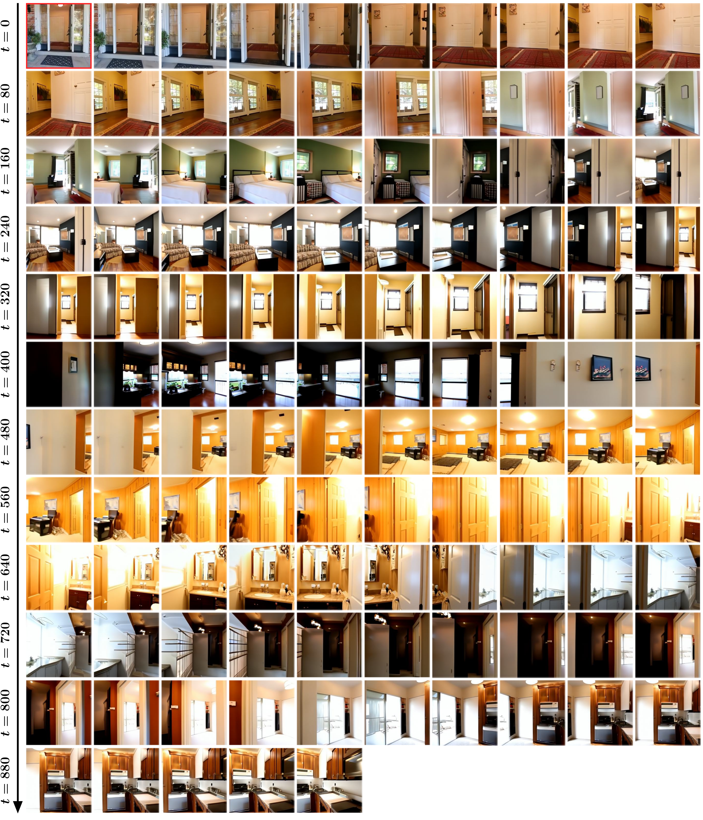
The 862-frame showcase starts from one image, but also uses an interactive user to choose camera motions after each coarse rollout. Six intermediate frames are then generated between successive coarse frames, giving a sevenfold interpolation interval. History guidance and a small noise-level stabilization help maintain consistency.
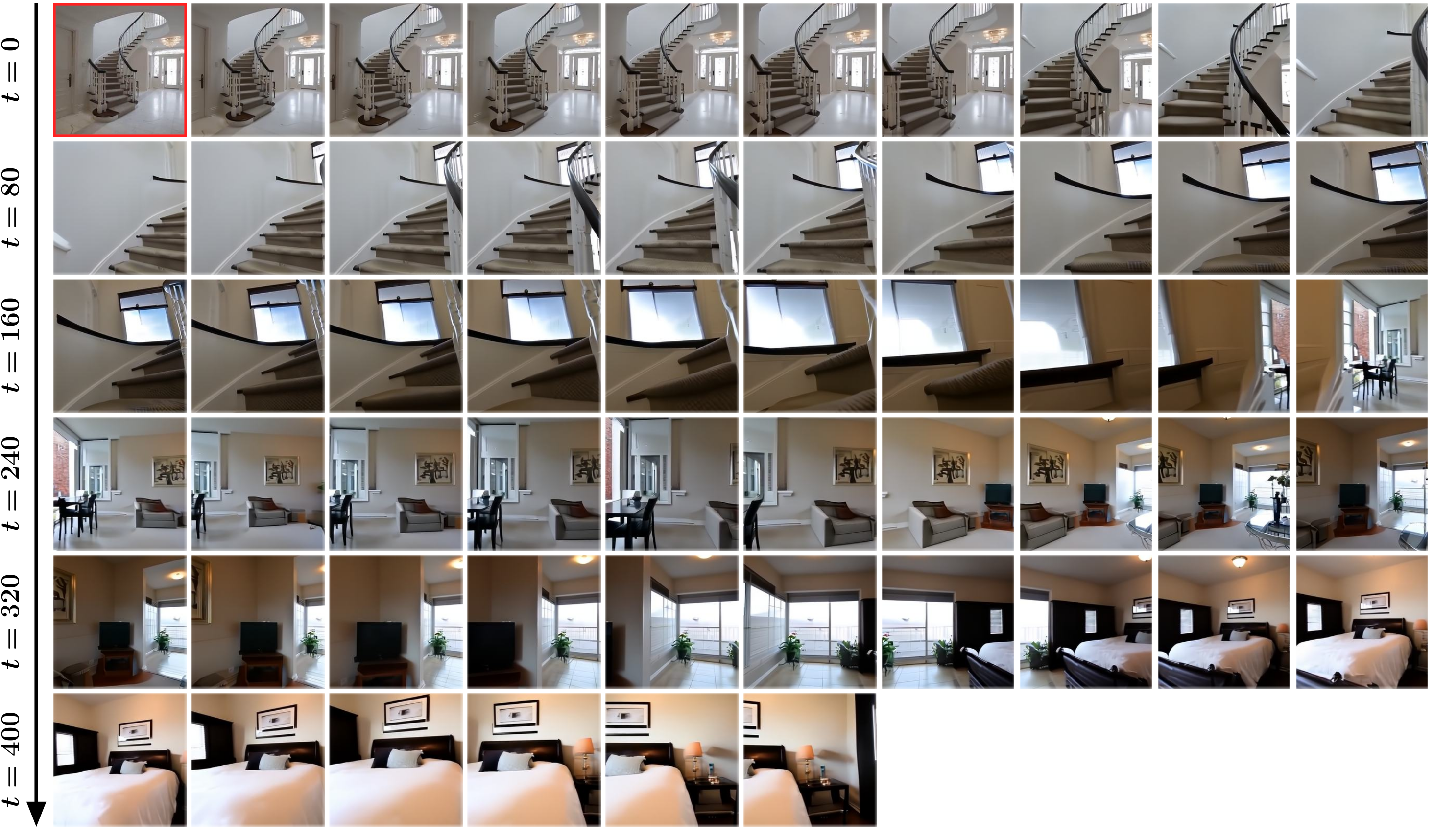
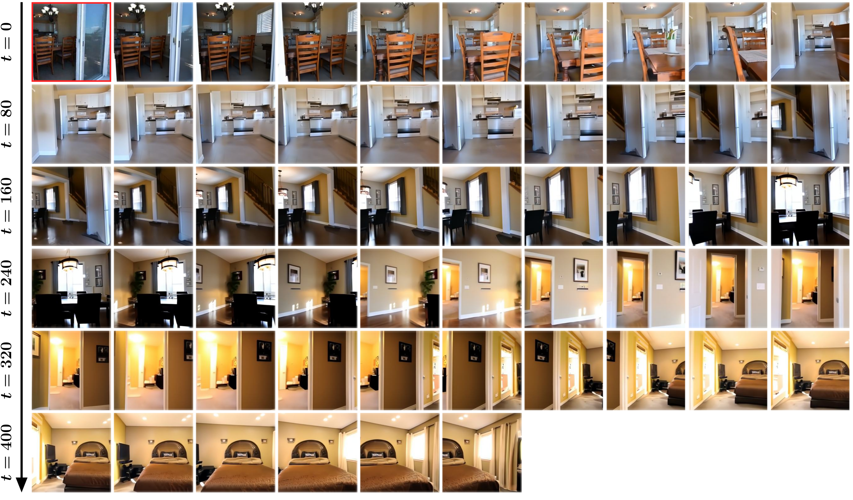
The long sample demonstrates extended guided synthesis, not 862 independently rolled-out frames from an image alone or autonomous navigation in a verified 3D world. Additional samples and a separate comparison without interpolation appear in the supplement.
7 Conclusion
DFoT makes the amount and form of historical conditioning available as sampling-time controls. The tested guidance mixtures improve selected quality, motion, and long-context outcomes, while fine-tuning can add this flexibility to a compatible pretrained model. Remaining limitations include guidance tradeoffs, finite context, additional score evaluations, qualitative long-rollout evidence, and the lack of a general guarantee for score composition.
Acknowledgements
The authors acknowledge support from the National Science Foundation, Singapore DSTA, IARPA through DOI/IBC, Amazon Science Hub, and the MIT–Google Program for Computing Innovation.
Impact Statement
Longer and higher-quality generated videos may support robotics and other applications, while also increasing the potential for harmful or misleading synthetic content. The authors call for responsible use; the paper does not experimentally evaluate misuse safeguards.
Appendix A Proofs, Explanations, and Extensions
The theory supplement develops a path-wise variational motivation, a Gaussian explanation of noise-conditioned attenuation, and an estimator-combination interpretation. It also supplies the complete sampler and implementation extensions. Formal statements and displayed derivations are retained verbatim below.
A.1 Derivation of an ELBO
A path specifies how each frame’s noise level increases from clean data to full noise. If the forward process and learned reverse process factor along that path, Jensen’s inequality yields a path-wise likelihood bound. Averaging over suitable monotone paths motivates a weighted denoising objective. No temporal causality is required for the index set.
The source notes that learned factorizations can be inconsistent across different paths and leaves enforcing consistency open. Its printed theorem writes a positive KL term with reversed arguments; the standard ELBO expansion instead subtracts KL(q‖p). The x-prediction corollary also prints a positive squared-error term in a likelihood lower bound. These formulas are preserved as published, so the summary treats them as an intended variational argument rather than a verified bound in the printed form.
Definition A.1 (Path).
We define a path as a sequence that begins at zero noise , and terminates at full noise .
Definition A.2 (Factoring Property).
We say that a model and forward process factor along a path if for any path, be a path, factors as , and factors as , with not depending on .
Theorem A.3.
Suppose that factor along a path . Then, for some constant not depending on , we have
Equation 7
| (7) |
Consequently, if denotes an expectation over paths along which factor, then
Equation
Corollary A.4.
Consider only paths for which entrywise, and for any and for which , increments by one.
Equation 8
| (8) |
and define , . Suppose that we parameterize , where further,
Equation
Further, let denote the -block component of , and suppose that if , then (i.e., if no denoising occurs, we do not re-predict the denoising). Then, for some distribution over paths along which satisfy the requisite factoring property, and for some constant independent of ,
Equation
where above, we define .
Remark A.5 (Factoring).
Observe that forward process in Equation 8 naturally factorizes across all the paths considered in Corollary A.4. While (by definition) factors across any single path , these factorizations may be inconsistent across paths. Enforcing some explicit consistency remains open for future work.
Equations Factoring, Definition A.2–Canceling
| (Factoring, Definition A.2) | ||||
| (Bayes’ Rule on ) | ||||
| (Telescoping) | ||||
| (Canceling) |
A.2 Understanding Frequency Guidance
The frequency argument assumes a linear Gaussian regression model with additive observation noise. In a Fourier basis, conditioning on a noisy observation shrinks directions with weak signal variance more strongly. When natural-signal power decays with frequency, this often suppresses high-frequency information.
This is a model-dependent attenuation argument, not a literal frequency cutoff. The printed Fourier definition, scaling identities, and covariance notation contain inconsistencies, including an invalid upper index in the cosine branch and conflicting noise-normalization factors. The original formulas remain intact; their qualitative interpretation is more reliable than using the printed expressions as implementation-ready identities.
Definition A.6.
Let denote the (real) discrete Fourier transform, specified by
Equation 9
| (9) |
We note that, by Parseval’s theorem, is an isometry:
Equation 10
| (10) |
Because is a bijective linear mapping, we identify it with an invertible matrix in .
Proposition A.7.
Let , and . Define , where is independent of . Define , and , and . Then,
-
-
-
The distribution of (or ) is
Equation 11
(11)
Interpretation in Terms for Frequency Attenuation:
With diagonal power-law spectral covariance, increasing observation noise suppresses more weak-variance directions. Gaussian noising itself has no preference for low frequency: that preference arises only when low frequencies have greater signal power. The retained Gaussian conditional lemma supplies the intended shrinkage calculation, with the source’s covariance and σ/σ² notation left unchanged.
Equation
Lemma A.8 (Gaussian Conditional Computation).
Let , and . Define , where is independent of . Set . Then, the distribution of is .
Equations 12
| (12) |
A.3 A Maximum Likelihood Interpretation for Score Addition.
The score-addition discussion assumes that several estimators have jointly zero-mean Gaussian errors around the same target score. Under a known nonsingular covariance, generalized least squares gives a covariance-weighted combination. Independent isotropic errors reduce this to inverse-variance averaging.
These are strong assumptions that are not established for scores conditioned on different video histories. The appendix presents the argument as intuition. Its general MLE formula omits the final design matrix in the matrix to be inverted, making the printed expression dimensionally problematic; the original expression is retained rather than silently repaired.
Assumption A.9 (Gaussian Errors).
We assume that, conditioned on , the errors form a Gaussian vector with mean zero and covariance .
Equations 13–15
| (13) |
| (14) |
| () | ||||
| () | ||||
| (15) |
Case 1: d = 1 ( 𝐱 is scalar) scores are independent.
For scalar, independent score errors with positive variances, the maximum-likelihood estimate is a convex combination with weights proportional to inverse variance. This special case explains why combining complementary estimators can help, without identifying optimal weights for history guidance.
Equation 16
| (16) |
Case 2: general d ( 𝐱 is scalar) scores are independent, and the errors s ^ i − s ⋆ have scaled identity covariance.
Independent vector errors with scaled-identity covariance yield the same inverse-variance weighting. A toy example then assigns disjoint error regions to individual estimators: averaging reduces squared error from 1/n to 1/n². The printed probability equality in that example is inconsistent, but the intended complementary-error illustration is straightforward.
Real guidance may use correlated estimators, negative unconditional coefficients, or weights that do not sum to one. The Gaussian averaging argument therefore does not prove that every guidance mixture is optimal or samples the exact desired conditional distribution.
Equations 17–20
| (17) |
| (18) |
| (19) |
| (20) |
A.4 Sampling with DFoT and History Guidance
Algorithm 1 preserves the full sampling procedure. At each denoising step, it computes an unconditional score and the requested history-conditioned scores, combines their differences, and advances a chosen score-based sampler. A partially masked history must actually be diffused to the supplied noise level; changing only the noise label would create a mismatched input.
Ordinary conditioning uses one clean history with weight one. Vanilla guidance increases that weight. Temporal guidance uses several clean subsequences. Fractional guidance combines the clean-history branch with a partially noised branch. The same interface supports extrapolation and interpolation by changing the observed/generated index sets.
A.5 Simplifying Training Objective
Independent noise works well for short latent sequences, but the authors observed degraded sampling with fifty latent frames. They propose reducing the task mixture by independently masking only the history positions that need flexibility, or sampling a history length before applying noise. The Minecraft setup uses a simplified objective; the broader alternatives are not systematically evaluated.
A.6 Causal Variant
A non-causal DFoT can generate causally by replacing unavailable future frames with independent noise, preventing conditioning on their actual contents. Partially masking known future frames instead permits controlled future information. This does not automatically provide the speed benefits of a causal architecture with key/value caching; those require additional design choices.
A.7 Incorporating Other Conditioning
History conditioning can coexist with text, action, or camera-pose conditioning. An existing external conditioning pathway need not be removed: the key modification is support for per-frame noise levels and the associated training objective. Large text-conditioned foundation-model adaptation is proposed rather than demonstrated here.
A.8 Extended Temporal History Guidance
Extended temporal guidance decomposes both the history and the generated frames into overlapping subsets. Scores are composed on shorter contexts and averaged frame by frame where generated subsets overlap. This is used in the unusual-camera-history experiment to reduce the distribution shift of the full input sequence.
Equation 21
|
|
(21) |
Supplementary Visuals
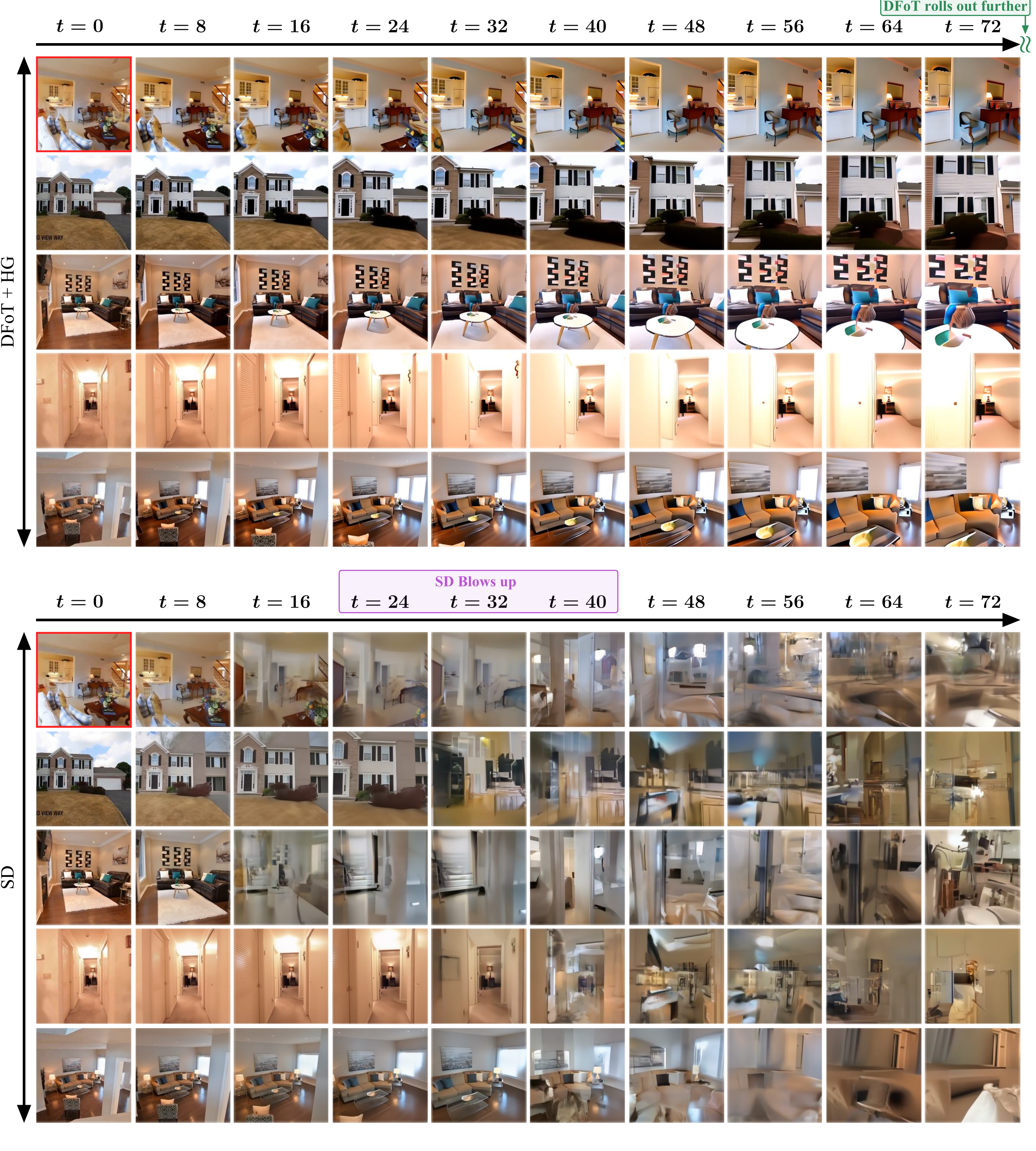
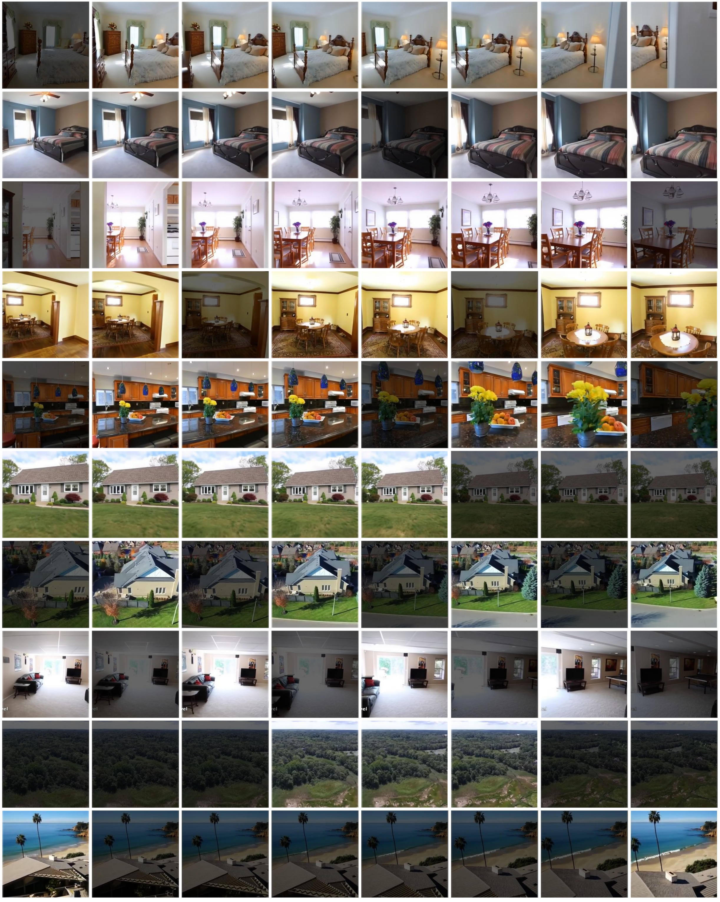
The retained supplementary grids show four long navigation rollouts, a rollout comparison, unusual-history interpolation, flexible observed subsets, guidance effects, Minecraft memory, and additional Kinetics samples. The HTML splits multipage figures and consequently uses different later figure labels from the PDF.
Appendix B Extended Related Work
The extended comparison distinguishes fixed-frame guidance from the arbitrary subsets and partial noise levels supported by DFoT.
B.1 History-conditioned Guidance
Earlier image-to-video and multiview systems use first-frame embeddings, channel concatenation, or fixed sets of masked conditioning frames. Some already process observed and generated images as one sequence, so that architectural idea alone is not unique to DFoT. The contribution combines flexible history with independent-noise training and richer score composition; the matched binary-dropout ablation tests one relevant alternative.
Appendix C Experimental Details
The protocol supplement specifies distinct datasets, model backbones, training schedules, conditioning schemes, and evaluation sample counts. These details matter when interpreting comparisons across experiments.
C.1 Datasets
Kinetics-600 contains diverse action clips at 128×128. RealEstate10K supplies 256×256 walkthrough images and camera poses. Minecraft provides 200,000 action-labeled navigation videos of 300 frames; its original 128×128 images are upsampled to 256×256, which does not add captured detail.
Fruit Swapping contains 300 complete swap demonstrations without disturbances and 300 short regrasp demonstrations without moving fruit between slots. Average lengths are about 540 and fifty frames. A 15 cm slot allows within-slot perturbations, so the evaluation requires combining memory of the initial arrangement with local recovery behavior not jointly demonstrated in a single training trajectory.
C.2 Implementation Details
Kinetics uses a chunk-wise VideoVAE and DiT; Minecraft uses an image VAE and DiT; RealEstate10K uses pixel-space U-ViT. Attention spans spatial and temporal tokens, with 3D rotary position embeddings and frame-specific adaptive normalization. Camera rays and actions supply additional conditioning. The robot model instead uses the attention U-Net listed in Table 2.
Models use cosine-based schedules, velocity prediction except x₀ prediction for the robot, dataset-specific loss reweighting, and AdamW training. Sampling uses fifty deterministic DDIM steps; multiple guidance branches are batched together, adding computation despite parallel evaluation. Robot tokens bundle fifteen actions with the next image.
The stated video training budget is about five days on twelve H100 GPUs per model; robot training takes four hours on four RTX4090s. Both implementation tables are retained completely. The Kinetics batch size is 192 in Table 2 but 196 in the resource discussion. Robot frame-skip wording also differs between the per-image description and the fifteen-action bundle shown in the table.
| Kinetics-600 | RealEstate10K | Minecraft | Imitation Learning | |
| VAEs | ||||
| Input | - | 256 | - | |
| Compression () | {1, 4}, 8 | 1, 8 | ||
| Latent channels | 16 | 4 | ||
| Training steps | 600k | 50k | ||
| Optimizer | Adam | Adam | ||
| Batch size | 64 | 96 | ||
| Learning rate | 1e-4 | 4e-4 | ||
| EMA | 0.999 | ✗ | ||
| VDMs | ||||
| Input | 256 256 | |||
| Latent | ✗ | ✗ | ||
| Frame skip | 1 | 10 Max | 2 | 15 |
| Backbone | DiT | U-ViT | DiT | Attention UNet |
| Patch size | 1 | 2 | 2 | 1 |
| Layer types | Transformer | Transformer | Attention, Conv | |
| Layers | 28 | 12 | 8 | |
| Hidden size | 1152 | 768 | 128 | |
| Heads | 16 | 9 | 12 | 4 |
| Training steps | 640k | 500k | 200k | 100k |
| Warmup steps | 10k | 10k | 10k | 10k |
| Optimizer | AdamW | AdamW | AdamW | AdamW |
| Batch size | 192 | 96 | 96 | 64 |
| Learning rate | 2e-4 | 5e-5 | 1e-4 | 5e-4 |
| Weight decay | 0 | 1e-2 | 1e-3 | 1e-3 |
| EMA | 0.9999 | 0.9999 | 0.9999 | ✗ |
| Diffusion type | Discrete | Continuous | Discrete | Discrete |
| Noise schedule | Cosine | Shifted Cosine | Shifted Cosine | Cosine |
| Noise schedule shift | ✗ | 0.125 | 0.125 | ✗ |
| Parameterization | ||||
| Sampler | DDIM | DDIM | DDIM | DDIM |
| Sampling steps | 50 | 50 | 50 | 50 |
C.3 Evaluation Metrics.
FVD compares generated and real video distributions in pretrained I3D feature space; it includes history frames here. VBench quality averages aesthetic and imaging scores, while consistency averages subject and background scores; dynamic degree measures motion. These scores evaluate generated videos without paired ground-truth comparison.
LPIPS is computed only on generated frames against their targets in highly constrained tasks. Low FVD or LPIPS does not establish physical correctness, and more motion is not universally better merely because dynamic degree increases.
C.4 Details on Video Generation Benchmark ( Section 6.2 )
The short-video benchmark predicts eleven frames from five observed frames. The latent model actually produces twelve and discards the last to match the standard sixteen-frame evaluation. FVD uses 50,000 generated videos and three random seeds.
The literature comparison mixes architectures and training regimes. The resource discussion compares parameter counts or FLOPs and batch sizes, not a fully matched total training-compute measurement. It says MAGVIT variants use comparable resources, while some other baselines use more; this is narrower than the introduction’s broad order-of-magnitude compute claim.
C.5 Details on History Guidance Experiment ( Section 6.3 )
For 64-frame Kinetics rollout, the model repeatedly conditions on two latent tokens and generates three more. Evaluation uses 1,024 videos. Guidance weights range from 1.0 to 4.0 in increments of 0.5; fractional guidance fixes the history noise level at 0.8. These results characterize the tested tradeoff curve.
C.6 Details on OOD History Experiment ( Section 6.4 , Task 1 )
RealEstate10K scenes are binned by camera-rotation range in ten-degree intervals. Up to 32 test scenes are sampled per bin, fewer in sparse bins. Histories contain four spaced frames and the model interpolates four target frames. Rotations above roughly 100° are uncommon in training, especially above 140°.
The temporal method combines two overlapping three-frame histories with weight two each and also overlaps three-frame generation subsets. The vanilla comparison uses the full history with weight two. Thus the result includes the extended generation-subset method, not solely a change in history length.
C.7 Details on Long Context Generation ( Section 6.4 , Task 2 ).
Minecraft training uses fifty subsampled frames with up to 25 history frames and an original-video stride of two. Evaluation starts with 25 context frames, then makes five 25-frame continuations, totaling 125 generated frames. Scores from 25-frame and four-frame histories receive equal weight, without subtracting an unconditional branch.
C.8 Details on Robot Imitation Learning ( Section 6.4 , Task 3 ).
The robot baselines diffuse actions and observations with current, short, or full histories. The protocol calls the short baseline two frames, while the results describe four. A full-history model can overfit to fruits being placed at slot centers; a short-history model can react locally but lose the intended final arrangement.
The reported composed policy uses one-frame, four-frame, and full-history scores with weights 0.45, 0.45, and 0.2. These sum to 1.1, so they are not a normalized convex average. The unconditional score is omitted. The observed failure modes motivate composition, but do not prove that a full-history policy is theoretically incapable of learning reactive behavior.
C.9 Details on Ultra Long Video Generation ( Section 6.5 ).
Long navigation first rolls out coarse frames: one observed image produces seven frames, then each iteration uses the last four to generate four more. A user supplies direction and distance after each iteration; these inputs become camera poses. Six frames are then interpolated between each adjacent coarse pair, using interpolated translations and SLERP rotations.
Rollout normally uses fractional guidance with weight four and history noise 0.4, switching to vanilla guidance for large direction or distance changes. Interpolation uses vanilla weight 1.5. Previously generated frames are marked slightly noisy at level 0.02 as an additional stabilization heuristic. The showcase’s length therefore reflects this entire pipeline.
Appendix D Additional Experimental Results
Additional experiments examine fine-tuning, binary dropout with guidance, long-context metrics, robot disturbances, and qualitative rollout behavior.
D.1 Additional Results on Fine-tuning to DFoT
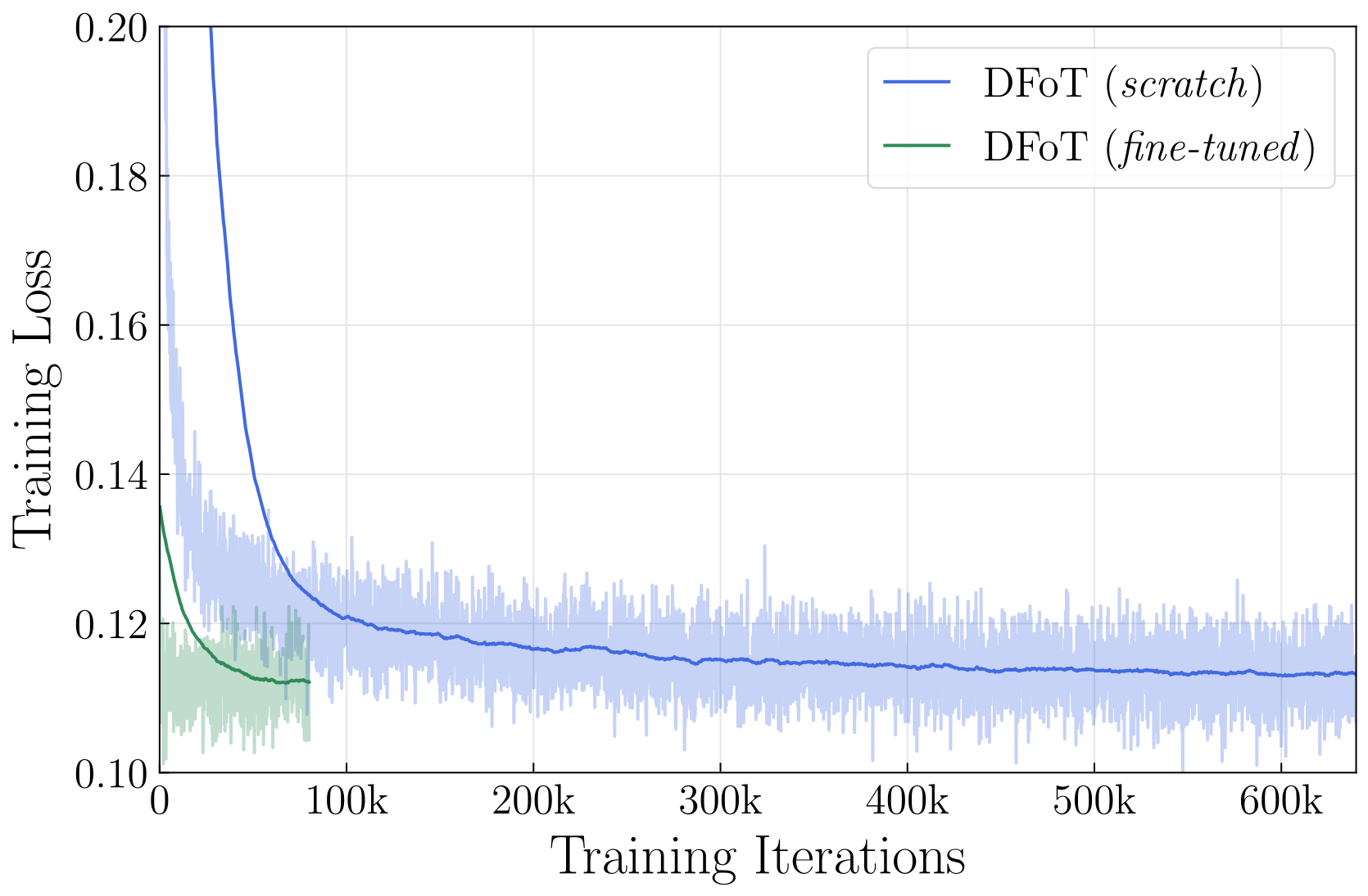
Fine-tuning a pretrained FS model for 80,000 steps gives lower training loss than the 640,000-step scratch model, but slightly worse FVD: 4.7 versus 4.3. At 40,000 steps the fine-tuned model scores 5.2. The claimed speedup concerns the additional fine-tuning stage and selected loss comparisons, excluding pretraining.
The authors attribute the lag in sample quality to slow exponential-moving-average adaptation. At 80,000 steps, removing EMA worsens FVD to 7.3. Predicting that additional training would surpass the scratch model is a hypothesis, not a reported result.
D.2 Ablation Study on Binary-Dropout Diffusion with Vanilla History Guidance
Binary dropout can use vanilla history guidance and reaches FVD 196.0 at its best tested weight, versus DFoT’s 181.6 with vanilla and 170.4 with fractional guidance. DFoT is not better at every tested weight: the text identifies an exception at 2.5. Fractional guidance additionally requires training on intermediate history-noise levels.
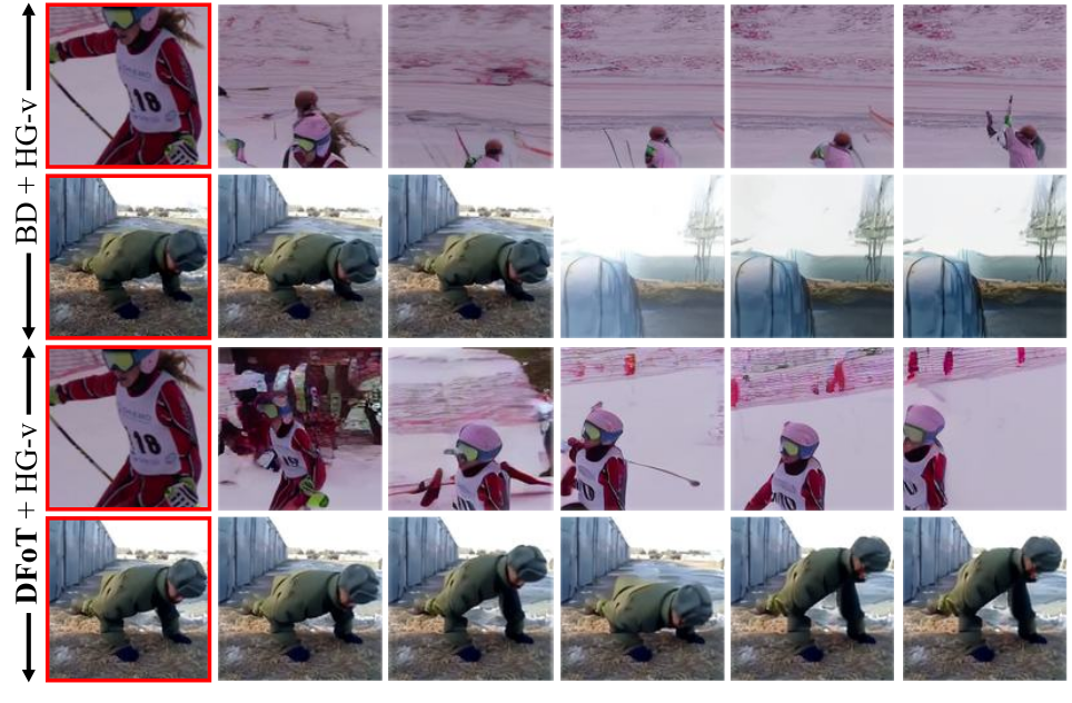
D.3 Detailed Results on Long Context Generation ( Section 6.4 , Task 2 )
Minecraft FVD uses 1,024 samples across all 125 generated frames. Temporal composition improves the reported metric from 97.625 to 79.19, and an example shows better retained detail. Action conditioning constrains variation, but this remains a dataset-specific result rather than a general guarantee of long-term consistency.
D.4 Detailed Results on Long-horizon yet Reactive Imitation Learning ( Section 6.4 , Task 3 )
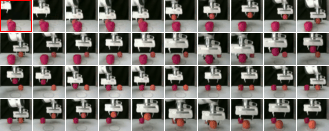
The main robot experiment randomizes the setup 100 times and reports 83% success for composed guidance. Short-context policies fail to maintain the overall plan; the full-history policy often grasps an old slot-center location after a fruit is moved. Occasional full-history recoveries are described, so the source does not justify assigning it an unreported zero success rate.
A harder intervention knocks fruit from the closing gripper; composed guidance succeeds in 28% of those reported trials, with the separate trial count unspecified. The results are consistent with combining memory and local recovery, but do not establish the internal mechanism of subtrajectory stitching.
D.5 Additional Qualitative Results
Additional grids preserve examples of base-model comparisons, arbitrary observed subsets, increasing guidance, unusual histories, and Minecraft generation. They illustrate specific successful and failed cases rather than proving uniform performance over every supported conditioning pattern.
D.6 Detailed results on Ultra Long Video Generation ( Section 6.5 ).
A separate straight-line navigation comparison omits interpolation for both models. SD visibly degrades around frame thirty in the displayed cases, while DFoT with guidance remains coherent beyond frame 72. The longer showcase samples contain 862, 917, and two 442-frame videos after the interactive rollout/interpolation pipeline.
These are qualitative examples, without an aggregate long-rollout failure rate or controlled human-navigation study. Their length exceeds the training clips, but this does not demonstrate persistent globally consistent scene geometry.