Stable port-Hamiltonian neural networks (sPHNNs) combine energy-based dynamics with a convex Hamiltonian whose minimum is fixed or learned. Their unforced dynamics remain bounded; strictly positive dissipation additionally gives global asymptotic convergence under the stated assumptions. Experiments include a spinning body, measured tank levels, and thermal surrogates. Knowing the equilibrium is especially valuable with sparse data; arbitrary driven inputs are outside the zero-input convergence guarantee.
1 Introduction
Physics-informed dynamics models can still extrapolate implausibly or become unstable. sPHNNs impose both an energy-balance structure and a Lyapunov-compatible Hamiltonian, avoiding projection-based stability enforcement. The approach targets systems with a single globally stable equilibrium in the modeled coordinates, including augmented latent states. Related foundations include Hamiltonian neural networks [16] and compositional port-Hamiltonian models [38].
2 Background
The background connects Lyapunov stability with the energy balance of port-Hamiltonian systems.
2.1 Stability of dynamical systems
Lyapunov stability keeps sufficiently perturbed trajectories near an equilibrium; asymptotic stability adds convergence. A positive-definite Lyapunov function with nonpositive time derivative establishes stability, while strict decrease and radial unboundedness support global asymptotic stability.
Equations 1–2
(1)
(2)
2.2 Port-Hamiltonian systems
The port-Hamiltonian form separates conservative dynamics through a skew-symmetric structure matrix, dissipation through a positive-semidefinite matrix, and external energy exchange through input ports. With no input, the Hamiltonian cannot increase. A damped rigid-body example illustrates this decomposition and the distinction between physical structure and additional stability constraints.
Equations 3–7
(3)
(4)
(5)
(6)
(7)
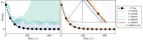
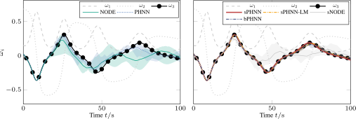
Figure 1: Spinning rigid body: Interquartile mean (lines) and range (shaded regions) of the energy
computed from the predicted states. Left: Models without stability bias; Right: Models with stability bias.
3 Stable port-Hamiltonian neural networks
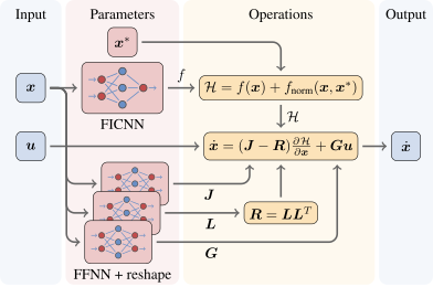
Neural networks parameterize the Hamiltonian and the structure, dissipation, and input matrices.
3.1 Stability of port-Hamiltonian dynamics
The theorem assumes zero input, a twice-differentiable convex Hamiltonian with zero value and gradient at the equilibrium, and a positive-definite Hessian there. It concludes a stable equilibrium and bounded trajectories. Positive-definite dissipation strengthens this to global asymptotic stability. Conservative or merely semidefinite dissipation does not establish attraction by this theorem.
Equations 8–9
(8)
(9)
3.2 Neural network model architecture
A fully input-convex network is normalized by subtracting its value and tangent at the chosen equilibrium, with an optional positive quadratic term ensuring the required curvature. If that term is omitted in practice, the needed positive-definiteness condition must be checked after training. Skew-symmetric and Cholesky parameterizations enforce the matrix structure. The equilibrium can be fixed from physics or optimized as a parameter. The convex network follows the input-convex architecture of Amos et al. [2].
(a)Computation graph.
(b)Composition of the total dynamics.
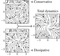
Figure 2: sPHNN model architecture: 2(a) Computation graph of stable port-Hamiltonian neural network. The FICNN parameterizing is normalized to obtain and the outputs of the FFNNs for , , and are reshaped to be skew-symmetric, lower triangular, and rectangular matrices, respectively. 2(b) Dynamics of a randomly initialized stable port-Hamiltonian neural network for , showing the built-in interpretability through the separation into conservative and dissipative dynamics.Equations 10–11
(10)
(11)
3.3 Training stable port-Hamiltonian neural networks
Derivative fitting is inexpensive but requires state-derivative labels and can accumulate rollout errors. Trajectory fitting differentiates through numerical integration, handles hidden augmented states, and costs more. The authors observe better optimization behavior with their stability bias, without claiming that it eliminates every possible training difficulty.
4 Experiments
Comparisons include unconstrained NODEs, ordinary PHNNs, bounded PHNNs without the convexity constraint, fixed-equilibrium sPHNNs, and learned-equilibrium sPHNN-LM. A projected stable-NODE baseline is used only for derivative fitting because its trajectory-fitting runs did not converge. Models use matched training steps and learning rates, with adaptive Tsit5 integration for prediction. The neural differential-equation and stable-dynamics baselines follow prior architectures [7], [27].
4.1 Spinning rigid body
Ten instances per model are trained from simulated angular-velocity derivatives. sPHNN, sPHNN-LM, and bounded PHNN track rotational energy best; unconstrained models show larger variability or unphysical energy behavior. The learned-equilibrium variant’s interquartile-mean equilibrium error is 0.010 in the reported coordinates.
4.2 Cascaded tanks
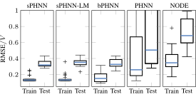
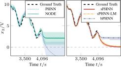
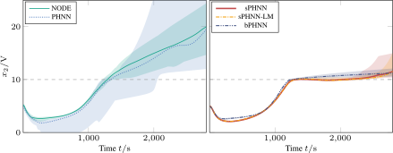
One 1,024-sample measured trajectory trains a two-state model of cascaded tanks, with only the lower tank observed. Across 20 instances, stability-biased models are more accurate and consistent. After the pump is switched off, fixed-equilibrium sPHNN relaxes to the expected zero level. Learned equilibria range from −0.196 to 0.432 V; boundedness alone does not ensure the physically correct final level.
Figure 3: Cascaded tanks: 3(a)RMSE of the models on training and test trajectory. 3(b): Predictions for the extended test trajectory. At , the pump is turned off. Lines correspond to the interquartile mean and shaded areas represent the interquartile range of the predictions from the model instances.
4.3 Thermal food processing surrogate
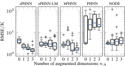
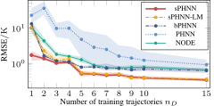
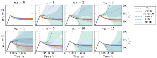
The food-processing surrogate predicts two internal temperatures from oven temperature using multiphysics simulation data. With two 280-sample training trajectories, added latent states help sPHNN while unconstrained models can become unstable in longer rollouts. Known equilibrium improves sparse-data performance over learning it. Table 1 reports median errors over 20 instances under noisy training; at 25% noise, test RMSE is 3.177 for sPHNN, 3.677 for sPHNN-LM, and 4.362 for NODE.
(a)Test root mean squared errors for training trajectories.
(b)Test root mean squared errors for augmented dimensions.
(c)Model predictions for different combinations of augmented dimensions and training data.
Figure 4: Thermal food processing surrogate: 4(a) and 4(b)RMSEs evaluated on test trajectories for various numbers of augmented dimensions and training trajectories .
4(c) Interquartile mean and range of the predictions for a custom test case. Top row: Varying number of augmented dimensions with fixed number of training trajectories. Bottom row: Varying number of training trajectories with fixed number of augmented dimensions. The time marks the length of the training trajectories.
Table 1: Median root mean squared error of instances per models using augmented dimensions, trained on noisy trajectories and evaluated on noise-free training and test sets.
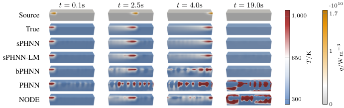
A simulated additive-manufacturing heat field is reduced to 40 temperature and 40 input coordinates. Models train on two of 25 parameterized trajectories using derivative fitting followed by trajectory fine-tuning. The reported sPHNN aggregate thermal error peaks below 30 K, while NODE and PHNN errors grow from unstable dynamics. This is surrogate modeling of simulation data, not a physical manufacturing deployment.
Figure 5: Heat source field and temperature field predictions on the cuboid domain for a test case with , . The instances selected for this evaluation resulted in the median test error for the corresponding model type. Colors are clipped to remain in the legend’s range.
5 Conclusion
Combining energy structure, equilibrium knowledge, and stability improves sparse-data extrapolation in these examples. The convex single-minimum model restricts representable dynamics and does not cover arbitrary multistability. Learning the equilibrium is possible, but supplying it from physical knowledge reduces data demands; multistable extensions remain future work.
Acknowledgments and Disclosure of Funding
The authors acknowledge DFG funding, CRC/TRR 361 CREATOR, Hessian.AI, and TU Darmstadt, along with colleagues who reviewed the manuscript.
Appendix A Proof of stability
The proof uses convexity and a strict local minimum to construct a linear radial lower bound on the Hamiltonian. This establishes global positive definiteness and bounded sublevel sets. The unforced energy-decrease condition then keeps every trajectory bounded; strictly positive dissipation and a unique stationary point yield global asymptotic convergence.
Equations A.1–A.8
(A.1)
(A.2)
(A.3)
(A.4)
(A.5)
(A.6)
(A.7)
(A.8)
Appendix B Experiment hyperparameters
Most experiments use two hidden layers of 16 units; the thermal-field surrogate uses 32. Tables retain training schedules, matrix parameterizations, instance counts, and computing costs. Representative sPHNN trajectory fitting takes 37.663 minutes versus 17.951 for NODE; single-trajectory integration is 0.365 versus 0.221 ms in the stated setup. Adaptive solver timings depend on the learned dynamics.
Table 2: Hyperparameters per experiment. TF and DF refer to trajectory and derivative fitting, respectively. The number of instances trained per model type is listed in the "# inst." column, and and denote the number of dimensions of state and input. The final three columns list the parametrization of the matrices for stable port-Hamiltonian neural network, stable port-Hamiltonian neural network-LM, bounded PHNN, and PHNN as either state-dependent matrices (s.) or constant matrices (c.).
Table 3: Representative computational costs for training and prediction. The top two rows report the training times for derivative and trajectory fitting, respectively. The bottom two rows show the time for a single derivative evaluation and a full trajectory integration using data and models from Section4.3.
Rigid-body data use ten initial angular velocities sampled from the unit cube, inertia diagonal (1, 2, 3), damping 0.01, and 50-second trajectories. The appendix compares extended angular-velocity predictions.
Figure C.1: Representative, extended training trajectory for spinning rigid body, including interquartile mean and range of model predictions for . Left: Models without stability bias; Right: Models with stability bias.
Appendix D Cascaded tanks data
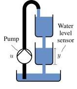
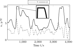
The tank benchmark contains separate 1,024-sample training and test trajectories with the same unknown upper-tank initial level. A ramped-input test probes overflow saturation at a 10 V sensor output. Stability-biased models capture saturation up to roughly 7 V pump input in the reported experiment; the unconstrained alternatives fail.
(a)Experimental setup
(b)Cascaded tanks training data (overflow highlighted).
(c)Saturation.
Figure D.1: Cascaded tanks: 1(a) System setup, 1(b) Training trajectory. 1(c) Predictions for a linearly increasing pump voltage. Due to an overflow, the true system exhibits a hard saturation at . Lines correspond to the interquartile mean, whereas shaded areas represent the interquartile range of the predictions from the model instances.
Appendix E Thermal food processing surrogate data
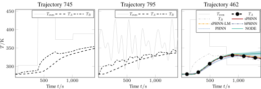
Thermal food data come from simulated chicken-breast heating, with center and near-surface probes. Training begins with trajectories 745 and 795; additional trajectories vary dataset size. Fifteen AP15 sequences form the test group. Scaling uses training data only and maps ambient temperature to zero.
Figure E.1: Left and middle: Training trajectories. Right: Exemplary test trajectory with interquartile mean and range of the model predictions for .
Appendix F Thermal field data
The thermal-field appendix describes dimensionality reduction and aggregate prediction errors.
F.1 Dimensionality reduction
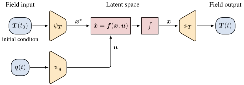
Separate singular-value decompositions of training temperature and heat-source snapshots define linear encoders and decoders. Latent temperature is shifted so equilibrium is at the origin, and zero heat input remains zero after encoding. Preliminary autoencoders compressed more strongly but extrapolated poorly with sparse data.
Equations F.1–F.6
(F.1)
(F.2)
(F.3)
(F.4)
(F.5)
(F.6)
Figure F.1: Model setup used in Section4.4. The initial temperature field and input field are mapped via encoders into the latent space, where the latent dynamics are integrated. Here, is used as a placeholder for a specific model, e.g., neural ordinary differential equation or stable port-Hamiltonian neural network. Finally, the predicted latent trajectory is mapped to the full-order field via the decoder .
F.2 Additional results
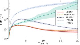
Across all 25 thermal trajectories, stability-biased models’ errors decrease as the system relaxes. Fixed-equilibrium sPHNN has the lowest peak error, nearly an order of magnitude below the bounded baseline in the reported plot. The learned-equilibrium variant is initially similar but retains a somewhat larger final offset.
Figure F.2: Interquartile mean and range of the RMSEs evaluated with all trajectories of the thermal field data.
57 references
[1]A. Abbasi, P. N. Kambali, P. Shahidi, and C. Nataraj.
“Physics-Informed Machine Learning for Modeling Multidimensional Dynamics”
In Nonlinear Dynamics, 2024
DOI: 10.1007/s11071-024-10163-3
[2]B. Amos, L. Xu, and J. Z. Kolter.
“Input Convex Neural Networks”
In Proceedings of the 34th International Conference on Machine Learning70, Proceedings of Machine Learning Research
PMLR, 2017, pp. 146–155
URL: https://proceedings.mlr.press/v70/amos17b.html
[3]M. Barreau and N. Bastianello.
“Learning and Verifying Maximal Taylor-neural Lyapunov Functions”
In arXiv e-prints, 2024
DOI: 10.48550/arXiv.2408.17246
[4]C. Beattie, V. Mehrmann, H. Xu, and H. Zwart.
“Linear Port-Hamiltonian Descriptor Systems”
In Mathematics of Control, Signals, and Systems30.4, 2018, pp. 17
DOI: 10.1007/s00498-018-0223-3
[5]L. Böttcher.
“Gradient-Free Training of Neural ODEs for System Identification and Control Using Ensemble Kalman Inversion”
In ICML Workshop on New Frontiers in Learning, Control, and Dynamical Systems, 2023
URL: https://openreview.net/forum?id=opPP65bJIN
[8]Y. Chen, Y. Shi, and B. Zhang.
“Optimal Control via Neural Networks: A Convex Approach”
In International Conference on Learning Representations, 2019
URL: https://openreview.net/forum?id=H1MW72AcK7
[9]A. Choudhary, J. F. Lindner, E. G. Holliday, S. T. Miller, S. Sinha, and W. L. Ditto.
“Forecasting Hamiltonian Dynamics without Canonical Coordinates”
In Nonlinear Dynamics103.2, 2021, pp. 1553–1562
DOI: 10.1007/s11071-020-06185-2
[10]M. Cranmer, S. Greydanus, S. Hoyer, P. Battaglia, D. Spergel, and S. Ho.
“Lagrangian Neural Networks”
In ICLR 2020 Workshop on Integration of Deep Neural Models and Differential Equations, 2019
URL: https://openreview.net/forum?id=iE8tFa4Nq
[11]S. Desai, M. Mattheakis, D. Sondak, P. Protopapas, and S. Roberts.
“Port-Hamiltonian Neural Networks for Learning Explicit Time-Dependent Dynamical Systems”
In Physical Review E104.3, 2021
DOI: 10.1103/PhysRevE.104.034312
[13]S. Eidnes, A. J. Stasik, C. Sterud, E. Bøhn, and S. Riemer-Sørensen.
“Pseudo-Hamiltonian Neural Networks with State-Dependent External Forces”
In Physica D: Nonlinear Phenomena446, 2023, pp. 133673
DOI: 10.1016/j.physd.2023.133673
[14]N. B. Erichson, M. Muehlebach, and M. W. Mahoney.
“Physics-Informed Autoencoders for Lyapunov-stable Fluid Flow Prediction”
In Machine Learning and the Physical Sciences (NeurIPS 2019), 2019
URL: https://arxiv.org/abs/1905.10866
[15]X. Glorot and Y. Bengio.
“Understanding the Difficulty of Training Deep Feedforward Neural Networks”
In Proceedings of the Thirteenth International Conference on Artificial Intelligence and Statistics9Sardinia, Italy: PMLR, 2010, pp. 249–256
URL: https://proceedings.mlr.press/v9/glorot10a.html
[17]E. Hairer, S. P. Nørsett, and G. Wanner.
“Solving Ordinary Differential Equations I: Nonstiff Problems”, Springer Series in Computational Mathematics 8
Heidelberg ; London: Springer, 2009
[18]Q. Hernández, A. Badias, D. Gonzalez, F. Chinesta, and E. Cueto.
“Structure-Preserving Neural Networks”
In Journal of Computational Physics426, 2021, pp. 109950
DOI: 10.1016/j.jcp.2020.109950
[19]P. Jin, Z. Zhang, I. G. Kevrekidis, and G. E. Karniadakis.
“Learning Poisson Systems and Trajectories of Autonomous Systems via Poisson Neural Networks”
In IEEE Transactions on Neural Networks and Learning Systems34.11, 2023, pp. 8271–8283
DOI: 10.1109/TNNLS.2022.3148734
[20]P. Jin, Z. Zhang, A. Zhu, Y. Tang, and G. E. Karniadakis.
“SympNets: Intrinsic Structure-Preserving Symplectic Networks for Identifying Hamiltonian Systems”
In Neural Networks132, 2020, pp. 166–179
DOI: 10.1016/j.neunet.2020.08.017
[21]M. Kannapinn, M. K. Pham, and M. Schäfer.
“Physics-Based Digital Twins for Autonomous Thermal Food Processing: Efficient, Non-Intrusive Reduced-Order Modeling”
In Innovative Food Science & Emerging Technologies81, 2022, pp. 103143
DOI: 10.1016/j.ifset.2022.103143
[22]M. Kannapinn, F. Roth, and O. Weeger.
“Digital Twin Inference from Multi-Physical Simulation Data of DED Additive Manufacturing Processes with Neural ODEs”, 2024
arXiv: https://arxiv.org/abs/2412.03295
[23]M. Kannapinn, M. Schäfer, and O. Weeger.
“TwinLab: A Framework for Data-Efficient Training of Non-Intrusive Reduced-Order Models for Digital Twins”
In Engineering Computations, 2024
DOI: 10.1108/EC23-0855
[25]D. Kingma and J. Ba.
“Adam: A Method for Stochastic Optimization”
In International Conference on Learning Representations, 2015
URL: https://arxiv.org/abs/1412.6980
[28]Z. Lai, C. Mylonas, S. Nagarajaiah, and E. Chatzi.
“Structural Identification with Physics-Informed Neural Ordinary Differential Equations”
In Journal of Sound and Vibration508, 2021, pp. 116196
DOI: 10.1016/j.jsv.2021.116196
[29]N. Lawrence, P. Loewen, M. Forbes, J. Backstrom, and B. Gopaluni.
“Almost Surely Stable Deep Dynamics”
In Advances in Neural Information Processing Systems33, 2020, pp. 18942–18953
[31]K. Lee and E. J. Parish.
“Parameterized Neural Ordinary Differential Equations: Applications to Computational Physics Problems”
In Proceedings of the Royal Society A: Mathematical, Physical and Engineering Sciences477.2253, 2021, pp. 20210162
DOI: 10.1098/rspa.2021.0162
[32]C. Legaard, T. Schranz, G. Schweiger, J. Drgoˇna, B. Falay, C. Gomes, A. Iosifidis, M. Abkar, and P. Larsen.
“Constructing Neural Network Based Models for Simulating Dynamical Systems”
In Acm Computing Surveys55.11New York, NY, USA: Association for Computing Machinery, 2023
DOI: 10.1145/3567591
[33]D. Liu and Y. Wang.
“Multi-Fidelity Physics-Constrained Neural Network and Its Application in Materials Modeling”
In Journal of Mechanical Design141.12, 2019, pp. 121403
DOI: 10.1115/1.4044400
[34]M. Lutter, C. Ritter, and J. Peters.
“Deep Lagrangian Networks: Using Physics as Model Prior for Deep Learning”
In International Conference on Learning Representations, 2019
URL: https://openreview.net/forum?id=BklHpjCqKm
[36]S. Massaroli, M. Poli, M. Bin, J. Park, A. Yamashita, and H. Asama.
“Stable Neural Flows”
In arXiv e-prints, 2020, pp. arXiv:2003.08063
DOI: 10.48550/arXiv.2003.08063
[37]H. Nakano, R. Ariizumi, T. Asai, and S.-i. Azuma.
“Model Estimation Ensuring Passivity by Using Port-Hamiltonian Model and Deep Learning”
Kumamoto, Japan: IEEE, 2022, pp. 886–891
DOI: 10.23919/SICE56594.2022.9905855
[38]C. Neary and U. Topcu.
“Compositional Learning of Dynamical System Models Using Port-Hamiltonian Neural Networks”
In Proceedings of the 5th Annual Learning for Dynamics and Control Conference211PMLR, 2023, pp. 679–691
URL: https://proceedings.mlr.press/v211/neary23a.html
[39]Y. Okamoto and R. Kojima.
“Learning Deep Dissipative Dynamics”
In Proceedings of the AAAI Conference on Artificial Intelligence39, 2025, pp. 19749–19757
DOI: 10.1609/aaai.v39i18.34175
[40]J. S. R. Park, S. W. Cheung, Y. Choi, and Y. Shin.
“tLaSDI: Thermodynamics-Informed Latent Space Dynamics Identification”
In Computer Methods in Applied Mechanics and Engineering429, 2024, pp. 117144
DOI: 10.1016/j.cma.2024.117144
[41]R. Pascanu, T. Mikolov, and Y. Bengio.
“On the Difficulty of Training Recurrent Neural Networks”
In Proceedings of the 30th International Conference on Machine Learning28.3, Proceedings of Machine Learning Research
Atlanta, Georgia, USA: PMLR, 2013, pp. 1310–1318
URL: https://proceedings.mlr.press/v28/pascanu13.html
[42]S. Ramasinghe, H. Saratchandran, V. Shevchenko, and S. Lucey.
“On the Effectiveness of Neural Priors in Modeling Dynamical Systems”
In ICML Workshop on New Frontiers in Learning, Control, and Dynamical Systems, 2023
URL: https://openreview.net/forum?id=7oe0lXarPm
[43]J. Rettberg, J. Kneifl, J. Herb, P. Buchfink, J. Fehr, and B. Haasdonk.
“Data-Driven Identification of Latent Port-Hamiltonian Systems”
In arXiv e-prints, 2024
DOI: 10.48550/arXiv.2408.08185
[44]S. M. Richards, F. Berkenkamp, and A. Krause.
“The Lyapunov Neural Network: Adaptive Stability Certification for Safe Learning of Dynamical Systems”
In Proceedings of the 2nd Conference on Robot Learning87PMLR, 2018, pp. 466–476
URL: https://proceedings.mlr.press/v87/richards18a.html
[47]M. Schoukens, P. Mattson, T. Wigren, and J.-P. Noël.
“Cascaded Tanks Benchmark Combining Soft and Hard Nonlinearities” CCBY-SA 4.0
4TU.ResearchData, 2020
DOI: 10.4121/12960104.v1
[50]N. Takeishi and Y. Kawahara.
“Learning Dynamics Models with Stable Invariant Sets”
In Proceedings of the AAAI Conference on Artificial Intelligence35.11, 2021, pp. 9782–9790
DOI: 10.1609/aaai.v35i11.17176
[51]A. J. van der Schaft and D. Jeltsema.
“Port-Hamiltonian Systems Theory: An Introductory Overview”, Foundations and Trends in Systems and Control 1, 2/3 (2014)
Boston Delft: Now, 2014
[54]J. Willard, X. Jia, S. Xu, M. Steinbach, and V. Kumar.
“Integrating Scientific Knowledge with Machine Learning for Engineering and Environmental Systems”
In Acm Computing Surveys55.4New York, NY, USA: Association for Computing Machinery, 2022
DOI: 10.1145/3514228
[55]H. Yu, X. Tian, W. E, and Q. Li.
“OnsagerNet: Learning Stable and Interpretable Dynamics Using a Generalized Onsager Principle”
In Physical Review Fluids6.11, 2021, pp. 114402
DOI: 10.1103/PhysRevFluids.6.114402
[56]Z. Zhang, Y. Shin, and G. Em Karniadakis.
“GFINNs: GENERIC Formalism Informed Neural Networks for Deterministic and Stochastic Dynamical Systems”
In Philosophical Transactions of the Royal Society A: Mathematical, Physical and Engineering Sciences380.2229, 2022, pp. 20210207
DOI: 10.1098/rsta.2021.0207
[57]Y. D. Zhong, B. Dey, and A. Chakraborty.
“Dissipative SymODEN: Encoding Hamiltonian Dynamics with Dissipation and Control into Deep Learning”, 2020
DOI: 10.48550/arXiv.2002.08860