Overview
At a glance
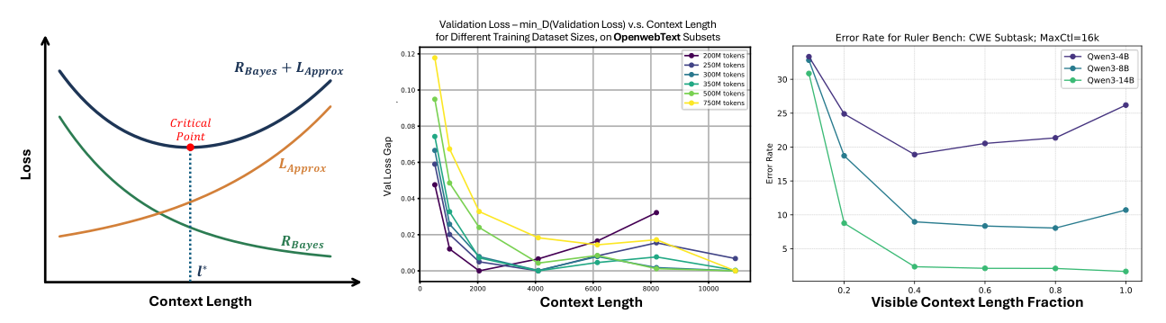
The paper explains context-length effects through two components: irreducible uncertainty with limited context and the trained model’s gap from that ideal predictor. It proposes intrinsic entropy of hidden representations as a proxy for information available from context. Experiments find entropy–loss correlations and intermediate best context lengths in selected training and retrieval settings. The framework is conditional on representation and scaling assumptions; it does not establish that every model or task has a finite optimal context length.
1 Introduction
More context can reveal useful evidence while also making prediction harder for a finite model trained on finite data. The authors connect these competing effects to latent-space entropy and dimension, extending earlier data/model scaling arguments Bahri et al., 2024. The contribution is an explanatory framework and a collection of measurements, rather than a new long-context architecture or an algorithm that automatically selects the best context for each input.
2 Assumptions, Deductions and Observations for Language Modeling
2.1 Preliminaries
2.1.1 Preliminary: Loss Decomposition
Expected next-token cross-entropy decomposes into the entropy of the ideal conditional predictor for visible length l plus the expected KL divergence from that predictor to the learned model. The first term is Bayes risk; the second is called approximation loss here and includes all learned-model mismatch. Bayes risk depends on the data distribution and visible information, not the particular model parameters. The exact decomposition should be distinguished from later assumptions about how each term changes with length.
Equation 1
| (1) | ||||
2.1.2 Preliminary: Intrinsic Space
Intrinsic space is a latent representation of contexts from which a decoder can predict the next token. In experiments, the authors use hidden features of trained networks as a proxy for this ideal space. Its geometry and entropy depend on the representation, model, and task; a hidden-vector entropy estimate is not automatically a model-independent information quantity.
2.1.3 Preliminary: Outlines
The analysis first relates ideal prediction loss to intrinsic entropy, then relates finite-data approximation to intrinsic dimension. Their proposed trade-off motivates context-length experiments during training and fixed-model inference. Appendix D formalizes the assumptions and gives geometric bounds.
2.2 Bayes Risk with context length: an Intrinsic Entropy perspective
2.2.1 Bayes Risk and Entropy in Intrinsic Space: derived from First Principles
The framework assumes that intrinsic entropy increases with context and approaches a finite limit. It further assumes that the reduction in next-token uncertainty is affine in intrinsic entropy, with a positive coefficient below one. Under that assumption, Bayes risk equals a constant minus a positive multiple of intrinsic entropy. The linear relationship is therefore an explicit premise of the theory, with experiments supplying evidence for its usefulness. Hidden states may also retain information needed for later tokens, so representation entropy is distinguished from next-token information. Continuous derivatives of integer context length use a smooth-extension convention.
Equation 2
| (2) | ||||
2.2.2 Bayes Risk and Intrinsic Entropy: Experiment Measurement
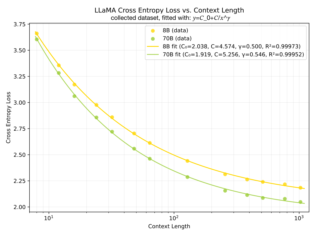
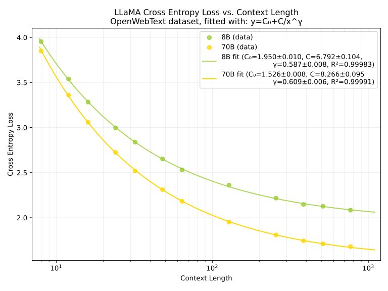
The authors use pretrained language-model cross-entropy as a proxy for ideal Bayes risk and fit a decaying power law C₀ + C/lᵞ. A good fit describes the measured models and corpora; it does not separately measure their remaining approximation loss or prove that they attain Bayes risk.
Equation 3
| (3) |
Experimentally measure Intrinsic Entropy using Gaussian-KDE
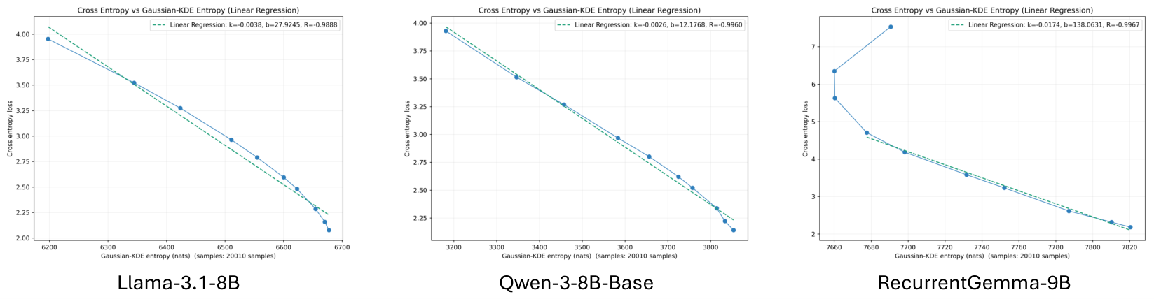
For each context length, at least 10,000 final-token, final-layer vectors are collected and Gaussian KDE estimates their representation entropy. On OpenWebText, Figure 2 reports loss–entropy correlations of −0.9888 for Llama-3.1-8B, −0.9960 for Qwen3-8B-Base, and −0.9967 for RecurrentGemma-9B after excluding three high-loss short-context points. The fitted slopes differ across models. These are strong within-experiment correlations; high-dimensional density estimation, feature scaling, and the selected exclusions limit interpreting them as exact or universal entropy laws.
Equation
2.3 Approximation Loss with Context Length: an Intrinsic Dimension Perspective
Approximation Loss in the Training Scenario
The proposed finite-data model is C₀ + A(l)/Dᵅ⁽ˡ⁾, with exponent approximately inversely related to intrinsic dimension. If longer context raises effective dimension, finite data can make approximation harder. Appendix D derives nearest-neighbor upper bounds under smooth-density, finite-negative-moment, and Lipschitz-decoding conditions, building on Sharma and Kaplan, 2022. An upper bound is not an exact loss law for a trained transformer, and length dependence of A(l) or other training effects must also be considered.
Equation 4
| (4) | ||||
Approximation Loss in the Inference Scenario
For a fixed pretrained model, the paper similarly proposes that longer visible context makes the ideal predictor harder to approximate. Harder tasks may increase this gap further. This is a modeling explanation for the observed failures, not a general theorem that every fixed model’s approximation error must grow monotonically with context.
3 Deduction: Optimal Context Length
A finite optimum can occur when the decreasing Bayes-risk slope and increasing approximation-loss slope cross. The authors argue that more training data or stronger models can move that balance to longer contexts, while tasks needing distant evidence can also benefit from longer inputs. Opposing monotonic trends alone do not guarantee a crossing, uniqueness, or its direction of movement; those conclusions require additional shape assumptions. The empirical optima below are measured within the tested context ranges.
Equation 5
| (5) |
3.1 Experimental Measurement of Optimal Context Length for Training
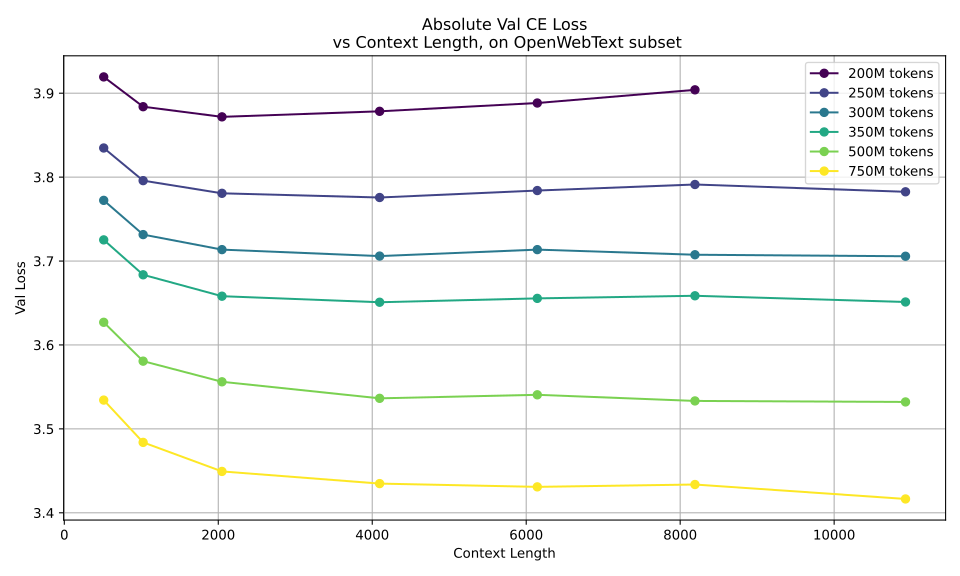
The training experiment uses a GPT-2-style network in nanoGPT Karpathy, 2022, with twelve heads and width 768 but only six transformer layers instead of twelve. Thus the named GPT-2-124M configuration is modified. The authors train with 200M, 250M, 300M, 350M, 500M, and 750M tokens and vary context length. Smaller-data curves exhibit minima followed by modest loss increases; the largest-data curve continues improving near the tested endpoint. Figure 1 subtracts each curve’s minimum for visibility, while Figure 15 retains absolute validation loss. Results support dataset-dependent context choices for this setup, rather than a universal cutoff.
3.2 Experimental Measurement of Optimal Context Length on Downstream Tasks
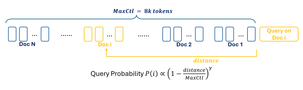
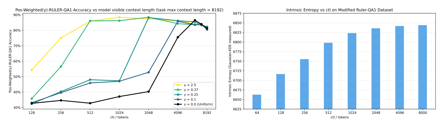
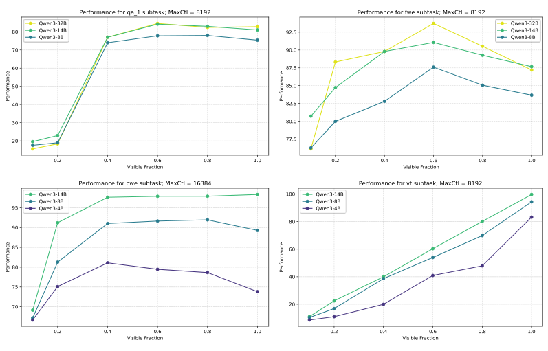
Fixed-model tests vary how much of a long input remains visible. Position-Weighted Ruler-QA1 modifies Hsieh et al., 2024 by sampling the answer-bearing paragraph with weight proportional to (1 − distance/maximum-length)ᵞ. Larger γ concentrates questions near the input end, while γ = 0 is uniform. In the tested Llama setup, more distant-information tasks generally favor longer visible contexts. Additional Qwen3 tasks show peaks for several question-answering and word-extraction settings, but variable tracking keeps improving across the tested range.
4 Proof of Concept with Synthetic Data
4.1 List of Points to prove
Synthetic parity tasks provide an analytically computable Bayes loss, allowing a clearer check of whether learned representations track information than is possible for natural language. The tests target loss–entropy linearity and agreement between measured hidden-space proxies.
4.2 Construction of Synthetic Data: the ‘position weighted multitask sparse parity’ dataset
Each task selects two fixed binary context positions and predicts their XOR. If either required bit is hidden, the best predictor incurs log 2 loss; otherwise the answer is known. Weighting task frequencies toward nearer positions produces a decreasing Bayes-loss curve resembling the fitted context power law. Figure 5 also illustrates why a single answer-token perplexity need not change equally when either of two relevant facts is removed. The main text alternates between 100 and 200 tasks: two tasks per maximum position from 11 through 60 specifies 100, while the task vocabulary is described as size 200. This reporting ambiguity is retained explicitly.
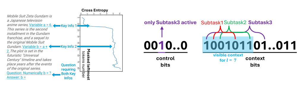
the answer for Subtask 1,2,3 is and respectively, but since the thrid bit is for control bits, only Subtask 3 is activated and the final answer is . However, for a model of context length , it cannot see the bit required by subtask 3, making it unable to predict the answer correctly.
Equation
4.3 Transformer-based Synthetic Model with Entropy Measurements
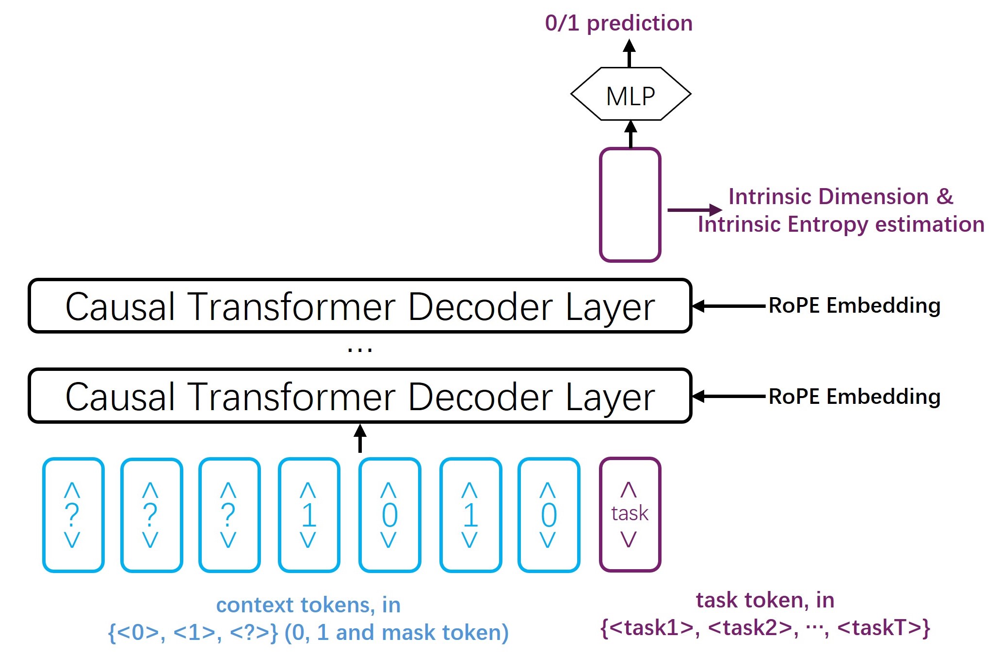
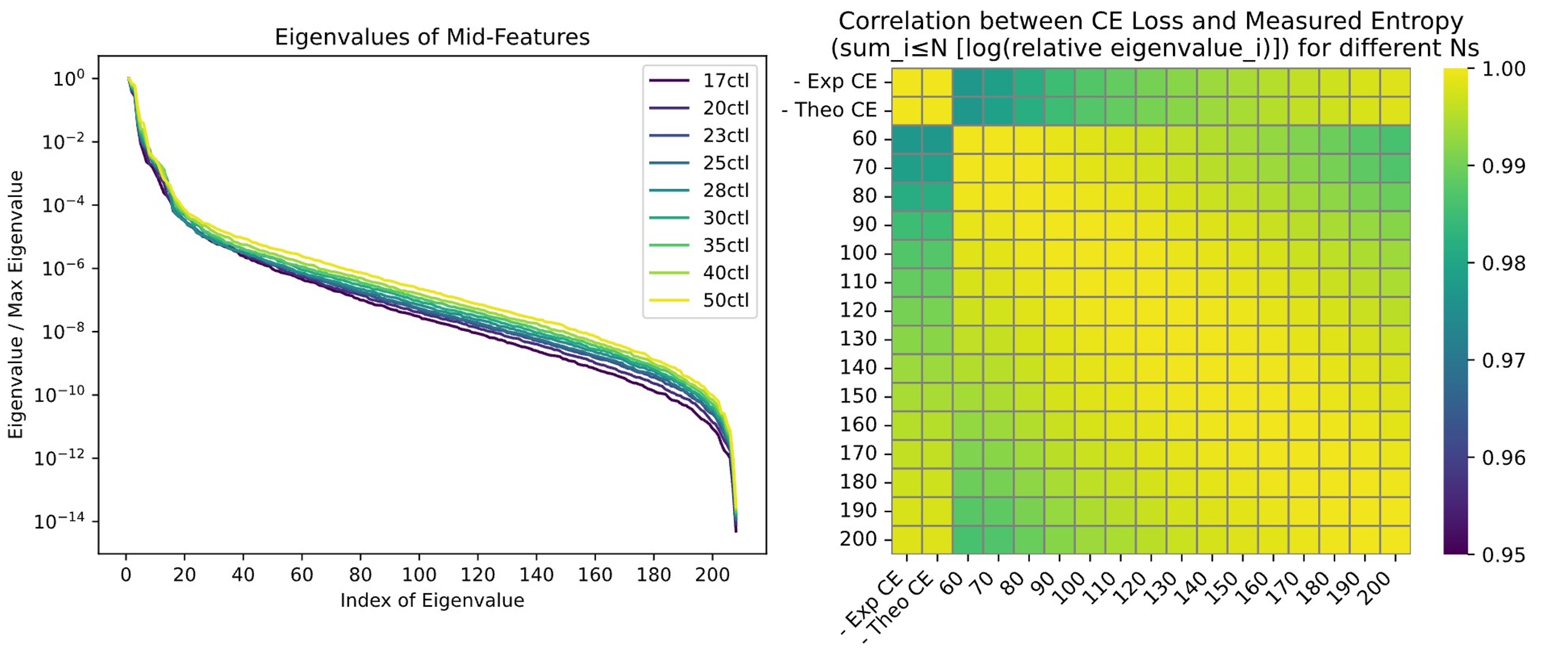
The synthetic transformer has three causal layers, width 208, feed-forward width 832, and RoPE base 4,000. Its sequence contains sixty context positions and a task token. Half of training examples are unmasked; the remainder hide a variable suffix using the source’s mask convention. The model is trained to approximate the known Bayes predictor. Eigenvalue spectra spread with greater visible context, and sums of log eigenvalues correlate strongly with measured and theoretical cross-entropy, especially when at least seventy dimensions are included.
4.4 Entropy in Intrinsic Space: Synthetic Dataset Validation
The synthetic model’s loss is close to its calculable optimum over the reported lengths, making this a useful controlled validation of the representation measurements. Both eigenvalue and density-based proxies show the expected association. The task frequencies and architecture are constructed to expose that structure, so the experiment does not independently establish the same assumptions for arbitrary natural-language problems.
5 Conclusion and Discussions
5.1 Conclusion
The work combines a Bayes-risk/approximation-error decomposition, representation-entropy correlations, and context sweeps showing intermediate optima in selected regimes. Its practical implication is to evaluate usable context jointly with data, model, and task, rather than assume that a larger accepted input always improves accuracy.
5.2 Limitations and Future Work
The authors acknowledge that the theory depends on its assumptions and that intrinsic geometry may depend on the model and prediction task. Further limits include approximating Bayes risk with imperfect models, high-dimensional entropy estimation, conditional geometric bounds, incomplete uncertainty reporting, and a limited set of training architectures and downstream tasks. The study motivates deeper theory and more general measurements; it does not provide an accuracy-preserving truncation rule for arbitrary prompts.
Appendix A Downstream Task
The appendix separates next-token prediction from downstream accuracy. It examines when a fixed model benefits from additional visible documents and whether representation entropy remains informative about that benefit.
A.1 Optimal Context Length on Ruler-QA: a Case Study
Ruler-QA1 inserts a SQuAD answer-bearing paragraph among other paragraphs, then varies the suffix visible to Llama-3.1-8B. The reported uniform-query curve peaks around 6k tokens before declining. Position weighting changes how often distant paragraphs matter. Appendix A mentions both 16k and 8k maximum-length constructions, while the main diagram and result plot use about 8k; the precise case-study settings should be checked in the released code before replication.
A.2 Intrinsic Entropy: a proxy of information learned by Language Model
KDE entropy is measured from late-token hidden states of truncated document collections. It generally rises with visible length, but it is independent of the query-position parameter γ, whereas accuracy depends on γ. It is therefore not a universal linear predictor of QA success. The authors interpret late-context accuracy deterioration as failure to approximate the task’s ideal predictor; the entropy correlation is strongest before that deterioration.
A.3 More experiments on RULER benchmark
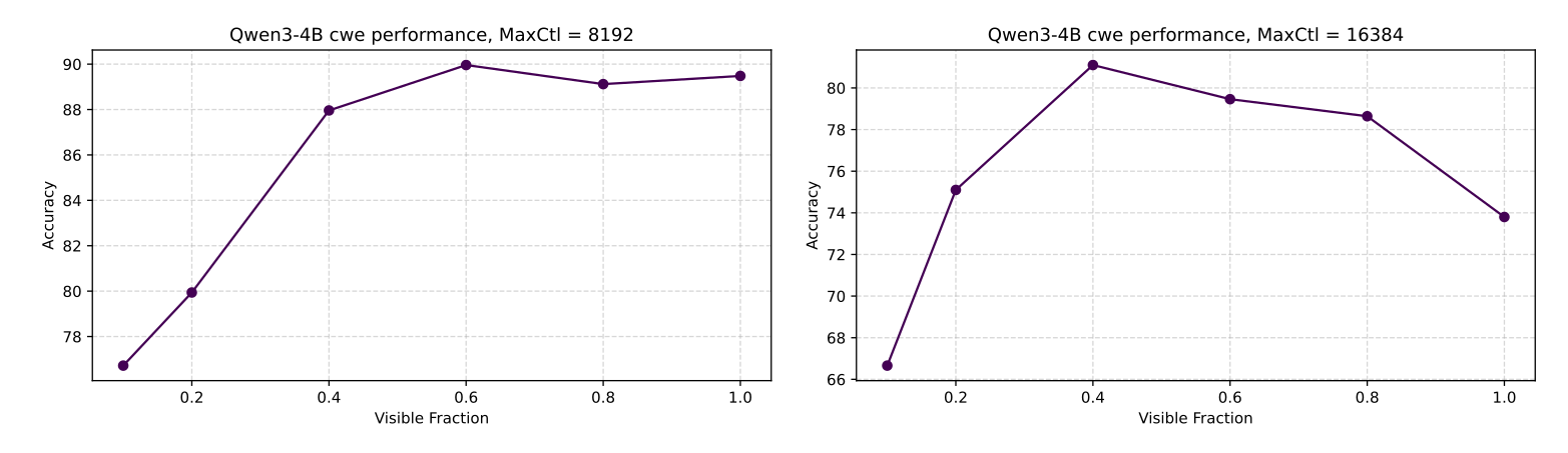
Qwen3 non-thinking chat models are tested on document QA, frequent-word extraction, common-word extraction, and variable tracking. Maximum length is 16k for common-word extraction and 8k for the other tasks. Figure 8 includes the four task plots; the additional Figure A.3-2 compares Qwen3-4B common-word extraction at 8k and 16k. Several models peak before full visibility, while variable tracking improves throughout. Larger models generally handle longer inputs better, and the 16k common-word task makes deterioration more apparent. These exceptions matter: a finite optimum is a measured phenomenon in some settings, not every curve.
Appendix B Definition and Properties of Cross Entropy loss
B.1 Definition of Cross Entropy Loss discussed in this work
The relevant cross-entropy averages negative log next-token probability over contexts and next tokens from the data distribution. It is the teacher-forced conditional prediction loss, rather than the cross-entropy of an entire generated context sequence. The appendix retains the full derivation connecting these definitions.
Equations 6
| (6) | ||||
B.2 Cross Entropy Loss for Language Model with Context Length l
When a model sees only the last l tokens, marginalizing the unavailable earlier context gives the true conditional distribution Pₗ. Expected cross-entropy then splits exactly into its conditional entropy plus expected KL(Pₗ ‖ Qₗ). Setting Qₗ = Pₗ identifies the limited-context Bayes risk and isolates the information lost by truncation.
Equations 7
| (7) |
Appendix C Experimentally measure next-token-prediction Information Entropy S n t p
C.1 PCA-based Information Entropy Estimation
The representation can encode information relevant to several future predictions, whereas the current output is a coarse-grained readout. The authors use correlations between cross-entropy and entropy proxies in different PCA subspaces to motivate a linear relationship. Correlation alone does not identify a unique predictive subspace or prove the assumed information mapping.
C.2 Gaussian-KDE based Information Entropy Estimation
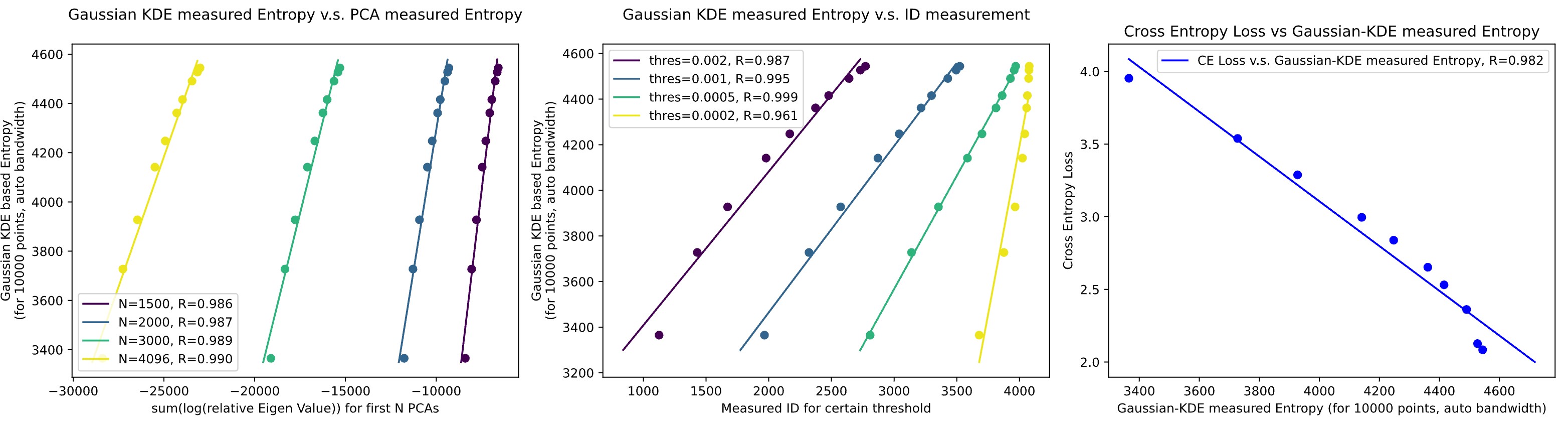
Figure 9 compares Gaussian-KDE entropy with PCA-based entropy, threshold-based dimension, and cross-entropy. It uses 10,000 samples and reported automatic bandwidth 0.997756. The estimators show similar trends on this experiment; the paper does not establish estimator accuracy across arbitrary hidden-vector distributions or bandwidth choices.
C.3 Synthetic dataset: Entropy in Intrinsic Space, and Entropy for output layer
In an idealized task-factorized representation, storing T independent binary task answers gives T log 2 entropy, while one binary output has log 2 entropy. This construction motivates proportional information scales. It relies on the assumed factorization and task structure, rather than proving that all learned latent dimensions encode equal independent information.
C.4 Details for synthetic data
The synthetic entropy experiment uses 10 million training examples, one million validation examples, and 125 epochs, with early-stopping patience 25 that is not triggered. Table 1 compares nine lengths from 17 to 50. Measured losses range from 0.4648 to 0.0613 and differ from calculated minima by at most about 0.0005 in the table. This directly supports near-Bayes behavior for that synthetic model over those lengths.
Equation
| Context Length | Model CE Loss | Minimum CE Loss Calculated |
|---|---|---|
| 17 | 0.4648 | 0.4643 |
| 20 | 0.3988 | 0.3988 |
| 23 | 0.3438 | 0.3437 |
| 25 | 0.3119 | 0.3116 |
| 28 | 0.2687 | 0.2686 |
| 30 | 0.2429 | 0.2429 |
| 35 | 0.1867 | 0.1864 |
| 40 | 0.1390 | 0.1387 |
| 50 | 0.0613 | 0.0612 |
Appendix D Definitions of Intrinsic Space and Derived Properties
This appendix makes latent-space properties explicit and derives conditional relationships. The distinction is between defining an ideal representation with these properties and showing how well actual network features satisfy them.
D.1 Formal Definitions of Intrinsic Space
Setup.
A finite vocabulary generates the set of finite contexts, and the data distribution defines its support. A mapping sends contexts of bounded length to a latent space.
Definition.
Predictive consistency requires a decoder that recovers the true next-token conditional distribution. Separate assumptions specify uniform predictive information per effective dimension or an affine entropy–prediction relationship. The geometric results also require a density with bounded gradient and a finite integral of q to the power 1 − ε. Table 2 maps each theorem to its assumptions. A finite vocabulary and a neural feature map do not by themselves establish the smooth-density or information-linearity conditions.
Equations 8–14
| (8) |
| (9) |
| (10) |
| (11) |
| (12) |
| (13) |
| (14) |
| Key Properties Assumed | Derived Results | |
| (Bahri et al., 2024)Theorem 2 | Bounded, Uniform Distribution, | Data Scaling for Approx. Loss |
| Lipschitz Differentiable | ||
| Theorem 1, 2 in Appendix D.2 | (Bounded,) Finite Negative Moment, | Data Scaling for Approx. Loss |
| (corr. to Section 2.3) | Lipschitz Differentiable | |
| Theorem 3 in Appendix D.3 | Predictive Consistency, | Bayes Risk for Ntp of varied Ctl |
| (corr. to Section 2.2.1) | Uniform Information Gain | (Intrinsic Dimension perspective) |
| Theorem 4 in Appendix D.4 | Predictive Consistency, | Bayes Risk for Ntp of varied Ctl |
| (corr. to Section 2.2.1) | Linear Entropy Relationship | (Information Entropy perspective) |
D.2 Derivation for Data Scaling for Approximation Loss
Theorem 1 bounds expected capped nearest-neighbor distance among D independent latent samples. Its proof uses a local density lower bound to control empty-ball probability, splits moderate/high-density from low-density regions, bounds the first with a tail integral, and controls the second using the finite negative moment. The resulting rate is D⁻¹ᐟᵈ when ε is large enough; otherwise a slower (log D/D)ᵋᐟ⁽ᵈ⁺¹⁾ term controls the bound. Every displayed proof equation is retained. The result concerns an expected geometric distance under stated regularity conditions, not measured transformer generalization by itself.
Equations 15–22
| (15) |
| (16) |
| (17) |
| (18) |
| (19) |
| (20) |
| (21) |
| (22) |
How large can ϵ be, for unbounded and bounded 𝒵 ?
A bounded support with density bounded away from zero satisfies stronger negative-moment conditions and permits the faster rate. Typical unbounded densities permit a smaller range of ε, giving a slower bound. This discussion explains the sensitivity to low-density tails; bounded support, compactness, finite measure, and a positive density lower bound should not be treated as interchangeable without further conditions.
Equation 23
| (23) |
From Nearest-Neighbour Distance to Approximation Loss
Theorem 2 combines the geometric result with Lipschitz control of decoder KL loss and bounded nearest-neighbor distance. It bounds expected nearest-neighbor predictive mismatch. The motivating connection to learned-model approximation additionally uses interpolation/Lipschitz assumptions from earlier work Bahri et al., 2024. It supplies a conditional scaling upper bound, rather than an equality or convergence guarantee for the training algorithm used in the experiments.
Equations 24–26
| (24) |
| (25) | ||||
| (26) |
Meaning of a finite ϵ -negative moment
The finite negative moment constrains low-density behavior. For 0 < ε < 1, it is algebraically related to finite Rényi entropy of order 1 − ε. The source also gives a low-density-volume interpretation. These formulas are preserved as the appendix presents them; the usable nearest-neighbor result still depends on its full smoothness, sampling, and support assumptions.
Equations 27–29
| (27) |
| (28) |
| (29) |
D.3 Derivation for Bayes Risk with Intrinsic Dimension Assumption
Under predictive consistency and uniform information gain, missing latent dimensions contribute a fixed amount to predictive KL divergence. Adding that divergence to irreducible full-context entropy yields Bayes risk affine in intrinsic dimension. A binary-integer example illustrates progressively revealing bits. This theorem derives the stated consequence of the information-per-dimension assumption, rather than establishing the assumption from language alone.
Equations 30–31
| (30) |
| (31) | ||||
D.4 Derivation for Bayes Risk with Information Entropy Assumption
Under predictive consistency and the zero-tolerance affine entropy assumption, conditional entropy directly becomes a constant minus s times latent entropy. The proof substitutes that assumed relationship into the conditional-loss identity. Nonzero tolerances or imperfect learned features would need additional error accounting.
Equations 32–33
| (32) |
| (33) | ||||
Appendix E More experiments of LLaMa on another dataset
The authors collect web text containing words they expect Llama’s pretraining filters to remove, then observe a similar context-loss power-law fit for Llama models. This is a supplementary corpus check. Such keyword selection does not independently verify that every passage or overlapping information was absent from pretraining, so the claimed unseen status remains an inference.
Appendix F Optimal Context Length for Two-needle-in-Haystack training: study on Synthetic Dataset
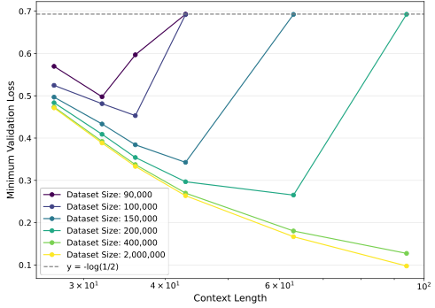
A longer synthetic parity setup uses more than 500 context bits, although most tasks depend on the first hundred. MLPs train at fixed dataset sizes until overfitting, and the best validation checkpoint is compared across context lengths. Many finite-data curves have an intermediate minimum that shifts outward with more examples. The experiment demonstrates the trade-off in this constructed problem, while some tested curves keep improving over the displayed range.
Appendix G Experiments on Other Language Models
Qwen3-8B-Base closely follows the loss–entropy trend. RecurrentGemma-9B has three short-context points with much higher loss; those are excluded from its linear regression and interpreted as poor approximation to the ideal predictor. The exclusion is part of the reported analysis, and the resulting correlation should not be described as fitting every tested context or architecture equally well.
Appendix H Eigenvalue-based Intrinsic Entropy Estimation
An alternative estimator uses hidden-feature covariance eigenvalues instead of kernel density estimation. Agreement between the two is examined empirically.
H.1 Bayes Risk vs. Context Length on OpenWebText
Llama-3.1 models on OpenWebText exhibit decreasing cross-entropy fitted by C₀ + C/lᵞ. Figure 12 retains both model curves and fits. The plotted quantity is actual model loss used as a Bayes-risk proxy, not an independently known entropy of natural language.
H.2 Eigenvalue-based Entropy Measurement
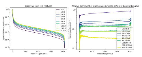
For at least 10,000 final-token vectors, PCA provides relative eigenvalues. The authors sum their logarithms as an entropy proxy, motivated by latent volume and Gaussian differential entropy. Figure 13 shows spectra and cross-length relative changes. This statistic depends on normalization, retained dimension, and covariance shape; constant scale conventions can shift it, and its interpretation as information requires the stated representation assumptions.
Equation
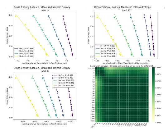
H.3 CE Loss vs. Eigenvalue-based Intrinsic Entropy
Figure 14 compares loss with log-eigenvalue sums over several leading subspaces and provides a correlation matrix. The reported correlations exceed 0.97 across many choices. This supports a stable empirical trend within the measured model/corpus, while highly correlated subspace statistics do not uniquely determine which features causally carry next-token information.
Equation
Appendix I Experiment Settings
I.1 Natural Language Data
I.1.1 Optimal Context Length Experiments
Training uses AdamW with learning rate 6 × 10⁻⁴, weight decay 0.1, and 1,000 warmup iterations. For a fixed token budget, context variants use the same iteration count, approximately token count divided by 0.1M. Long OpenWebText documents are selected before splitting; validation contains 134M tokens. The paper reports roughly 300 GPU-hours on eight AMD MI250X devices for the context sweep. Figure 15 preserves absolute losses, including cases where changes between long contexts are small; repeated-seed uncertainty is not shown.
I.1.2 Intrinsic Dimension Experiments
The representation measurements use 10,000 sufficiently long OpenWebText samples, final-token features from Llama-3.1-8B’s last layer, and about 100 reported GPU-hours on MI250X hardware. These details describe the empirical proxy, not a direct measurement of a unique language data manifold.
Appendix J Related Work
J.1 Enlarging Context Length for LMs
Related approaches extend usable context through rotary position embeddings, longer-context training, cache compression, linear attention, recurrent or state-space models, and staged short-to-long training Su et al., 2023; Gu and Dao, 2024. Those methods change representation or computation, whereas this paper studies the observed relation between context and prediction quality.
J.2 Irrelevant Long Context hurts performance of LMs
Earlier two-needle and retrieval studies show that irrelevant surrounding material can hurt performance Levy et al., 2024. The present analysis also considers contexts containing additional useful evidence, so relevance alone does not guarantee that a particular trained model will exploit the extra input.
J.3 Long Context in another field: Time Series Forecasting
Prior time-series work finds an optimal look-back horizon that grows with dataset size Shi et al., 2024. This motivates the language experiments, but the analogy is not itself evidence that the same quantitative law holds across domains.
J.4 Related Theories for Scaling Laws
The discussion situates the framework alongside empirical scaling laws, manifold-dimension explanations, feature-quantization models, and intrinsic-dimension accounts of adaptation. Its added focus is context length and the information represented by hidden states, with model/data scaling providing supporting assumptions.
Appendix K Intrinsic Dimension perspective: measurements in Intrinsic Space
This appendix develops an alternative dimension-based account and connects it to the entropy measurements through eigenvalue spectra.
K.1 Bayes Risk from an Intrinsic Dimension perspective: Assumptions
Assumptions posit a finite limiting effective dimension, growth with context, and constant predictive information per dimension. They imply an affine decrease of Bayes risk with effective dimension. This is stronger than simply observing that more context can provide more information; its relevance is assessed through the following measurements.
Equation 34
| (34) | ||||
K.2 Experimentally measure Intrinsic Dimension using PCA
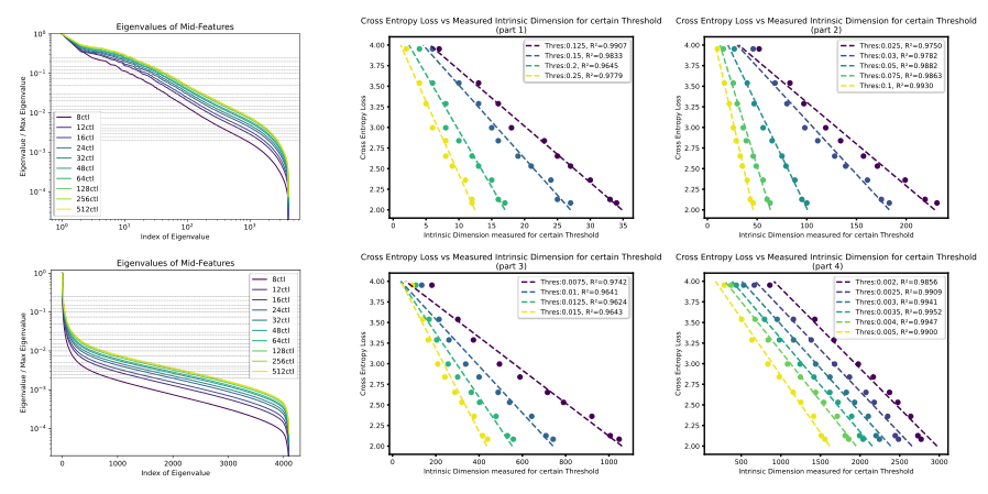
PCA dimension is estimated by counting eigenvalues above a relative threshold. Thresholds from 0.002 to 0.25 produce different numerical dimensions but broadly linear relations with loss. Figure 16 retains spectra under two axis scalings and all threshold/loss plots. This is a threshold-dependent effective dimension, not a threshold-free topological dimension of language.
Equation
K.3 MLP-based Synthetic Dataset: Intrinsic Dimension Experiments
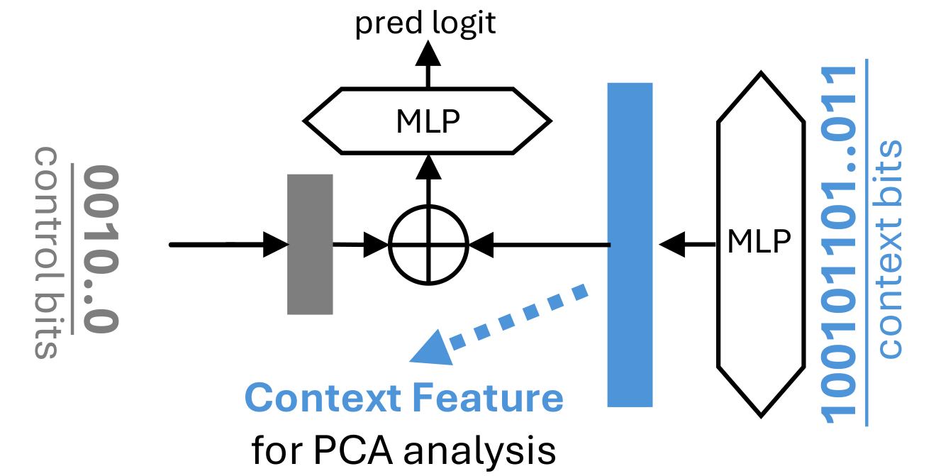
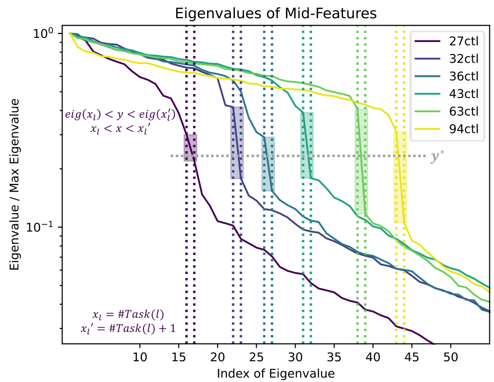
An MLP separates context encoding from task selection, allowing PCA on the context feature. The constructed tasks assign one information unit per visible subtask, and fitted context–dimension and context–loss power laws report R² = 0.9997. Measured representation spectra show a cutoff related to visible tasks despite a fixed internal width of eighty. Figures 17–18 preserve the architecture, every spectrum, and threshold intervals. The extremely close fitted relationships reflect this deliberately structured test rather than a general estimate for natural language.
K.4 Bridging the gap between Intrinsic Dimension explanation and Intrinsic Entropy explanation
If high-index eigenvalues share approximately the same exponential decay rate and differ mainly by a context-dependent scale, log-eigenvalue entropy and threshold-counted dimension both become affine functions of that scale’s logarithm. This explains why their measured relationships with cross-entropy can align, with slope tied to subspace dimension and decay rate. The derivation applies to the fitted spectral regime, not every possible representation distribution.
Equations 35–36
| (35) | ||||
| (36) |
Appendix L Disclosure of LLM Usage
The authors disclose using language models only to polish the writing.