Literature
Display
← All papers

s1: Simple test-time scaling

Niklas Muennighoff · Zitong Yang · Weijia Shi · Xiang Lisa Li · Li Fei-Fei · Hannaneh Hajishirzi · Luke Zettlemoyer · Percy Liang · Emmanuel Candès · Tatsunori Hashimoto

· EMNLP 2025 ↗

Language models14 min text · CondensedOriginal paper ↗
Contents

At a glance

s1 combines supervised fine-tuning of Qwen2.5-32B-Instruct on 1,000 selected examples with budget forcing at inference time. A delimiter ends reasoning at a chosen limit; suppressing it and inserting “Wait” can extend reasoning beyond the model’s usual stopping point. On AIME24, the reported score rises from 50.0% to 56.7%—two additional correct answers among thirty questions.

The final fine-tuning run takes about seven H100 GPU-hours, but relies on a pretrained model and a much larger pool of teacher-generated examples plus filtering. The revised supplement adds s1.1, trained on the same questions with DeepSeek-r1 traces, and reports better math/science results. Longer reasoning is useful over a tested range, but can plateau, loop, or exceed the context window.

1 Introduction

Test-time scaling spends extra inference computation to improve an answer. This paper asks how little additional training and decoding machinery is needed to obtain a useful scaling curve. It distills a small selected subset of Gemini-generated reasoning into an existing instruction-tuned model, then explicitly controls how long that model reasons.

The contributions are the s1K selection procedure, a simple stopping/continuation intervention, and ablations of both. The results demonstrate a practical recipe on the evaluated math and science tasks, rather than a general law that more reasoning always helps. Code, weights, and data are available in the original repository.
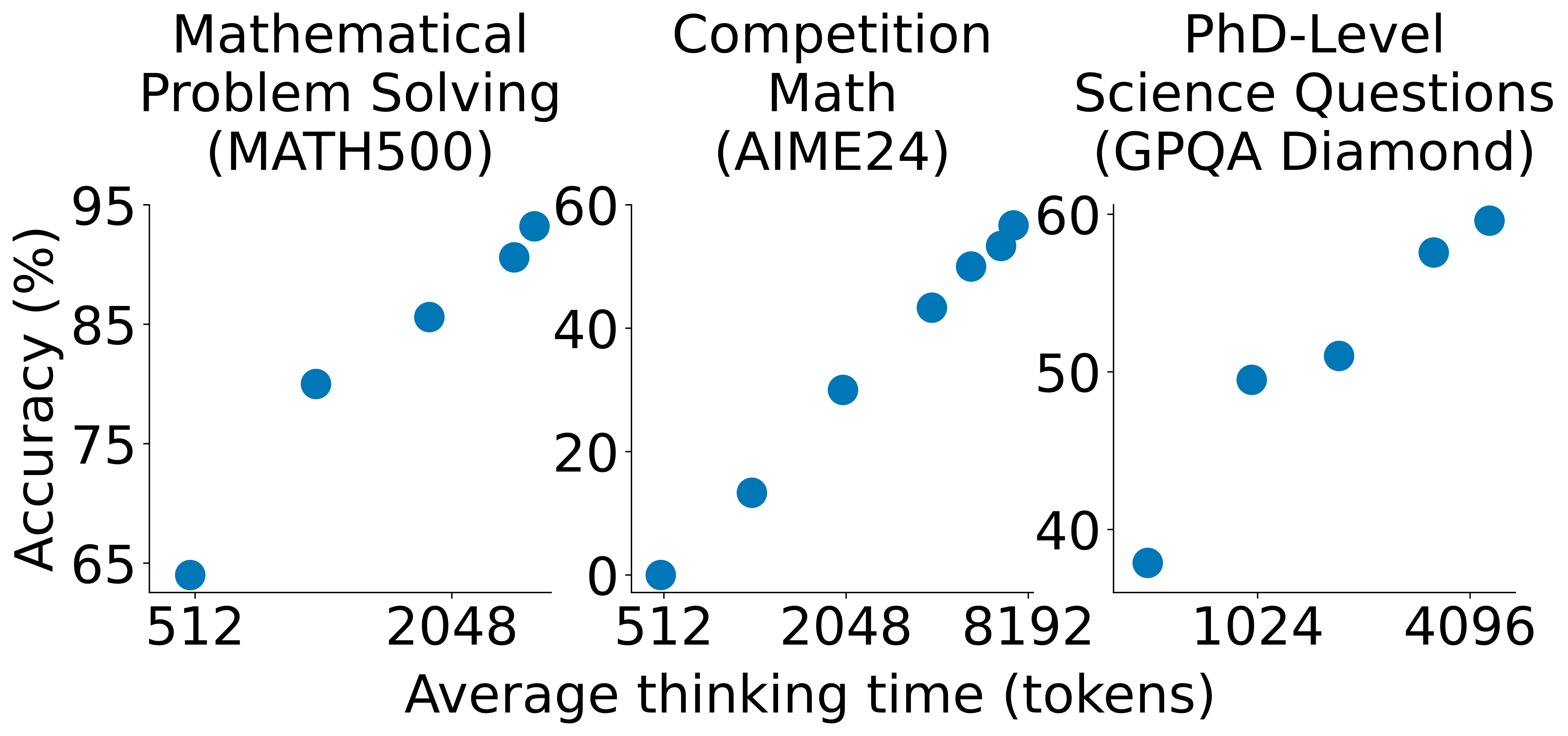
Original figure
Figure 1: Test-time scaling with s1-32B. We benchmark s1-32B on reasoning-intensive tasks and vary test-time compute.
Original figure
Original figure
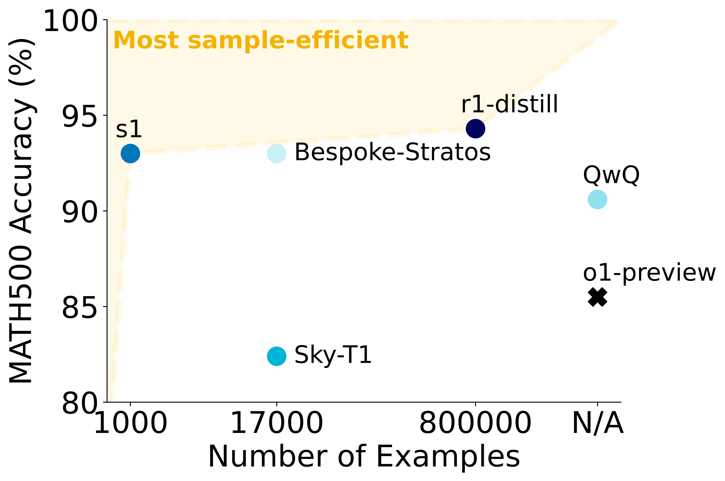
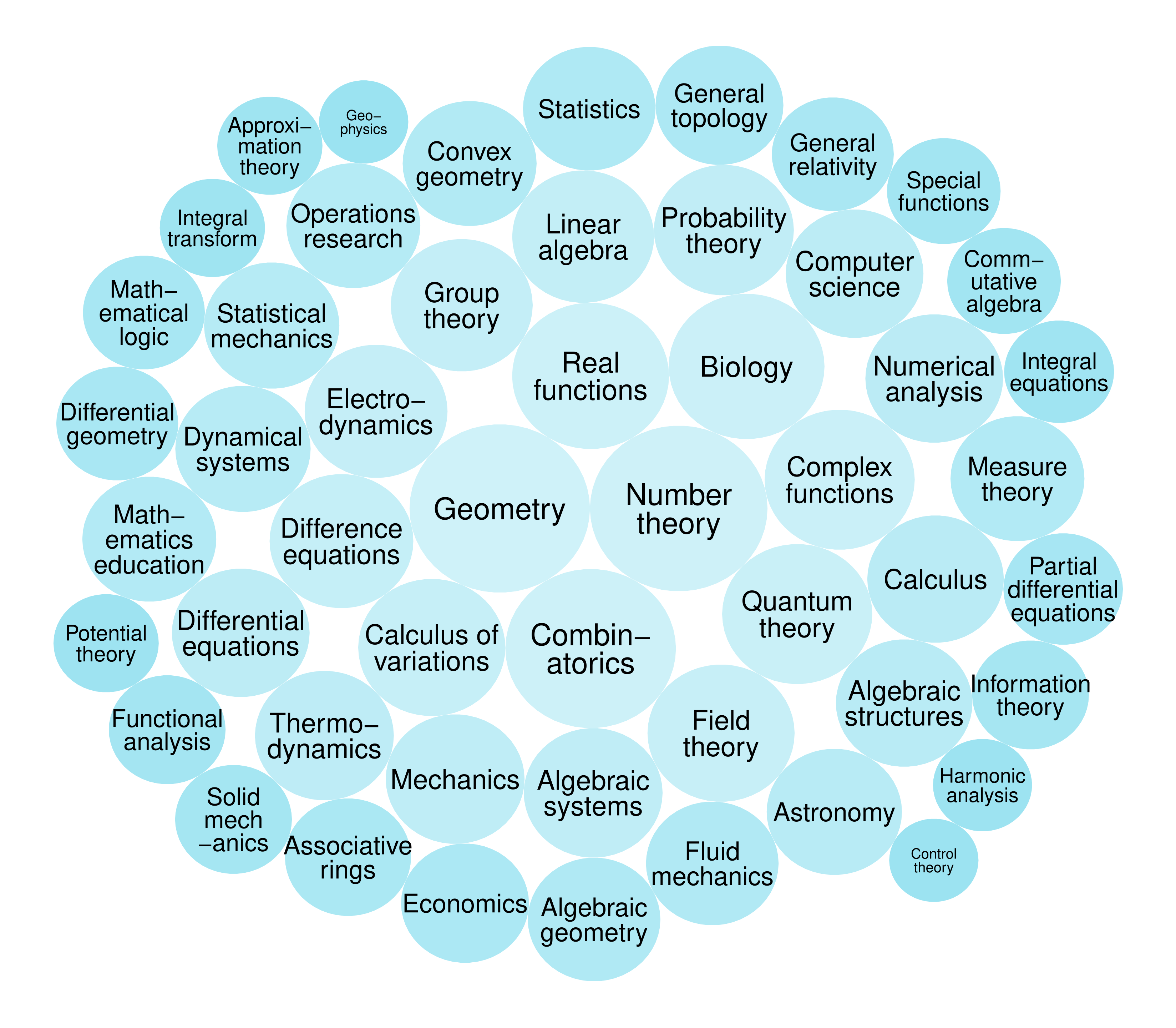
Figure 2: s1K and s1-32B. (left) s1K is a dataset of 1,000 high-quality, diverse, and difficult questions with reasoning traces. (right) s1-32B, a 32B parameter model finetuned on s1K is on the sample-efficiency frontier. See Table 1 for details on other models.

2 Reasoning data curation to create s1K

Data construction first gathers a broad pool of questions and teacher responses, then selects a small fine-tuning set using quality, difficulty, and topic diversity.

2.1 Initial collection of 59K samples

The initial pool contains 59,029 questions from sixteen sources. Sources are inspected for usable formatting, substantive reasoning demands, and topical coverage. Gemini Flash Thinking generates a reasoning trace and response for each attempted question; failed calls and malformed examples are subsequently removed.

Curation of existing datasets

The largest sources are NuminaMATH, MATH, OlympicArena, OmniMath, and AGIEval. Other sources contribute historical AIME questions, coding tasks, university-level science, and crosswords. The complete source table retains counts and average teacher-trace lengths.

New datasets in quantitative reasoning

Two smaller collections add 182 Stanford statistics qualifying-exam problems and 23 hard quantitative-interview brain teasers. The questions and reference solutions seed teacher generation; they do not guarantee that the generated reasoning is correct. Evaluation questions are screened with an eight-gram overlap check, and duplicates are removed.

2.2 Final selection of 1K samples

The goal is a compact final training set, not a minimal total data-generation budget. The pipeline uses teacher generation and model-based filtering over tens of thousands of candidates to choose 1,000 examples.

Quality

Removing API failures leaves 54,116 examples. Filtering formatting problems, unsupported image references, and similar defects leaves 51,581. The authors seed the final selection with 384 examples from sources judged particularly useful before filling the remaining slots through difficulty and diversity selection.

Difficulty

Qwen2.5-7B-Instruct and Qwen2.5-32B-Instruct attempt the questions; Claude grades their answers against references. Questions solved by either model are excluded from the difficult candidate pool, leaving 24,496. Longer teacher traces serve as a second difficulty proxy. These criteria are tailored to the Qwen models and can also select verbose or mistaken traces.

Diversity

Claude assigns domains using the Mathematics Subject Classification taxonomy. Sampling alternates uniformly chosen domains with length-favoring selection inside each domain until the final set is full. The text reports fifty domains, while the summary table labels the total fifty-one; the table’s listed categories plus its remaining-domain count also imply fifty.

Teacher correctness is not required for every selected example. Claude 3.7 later grades 53.6% of s1K and 63.0% of s1K-1.1 as correct. These are automated assessments, and the complete examples intentionally retain mistakes and backtracking.

3 Test-time scaling

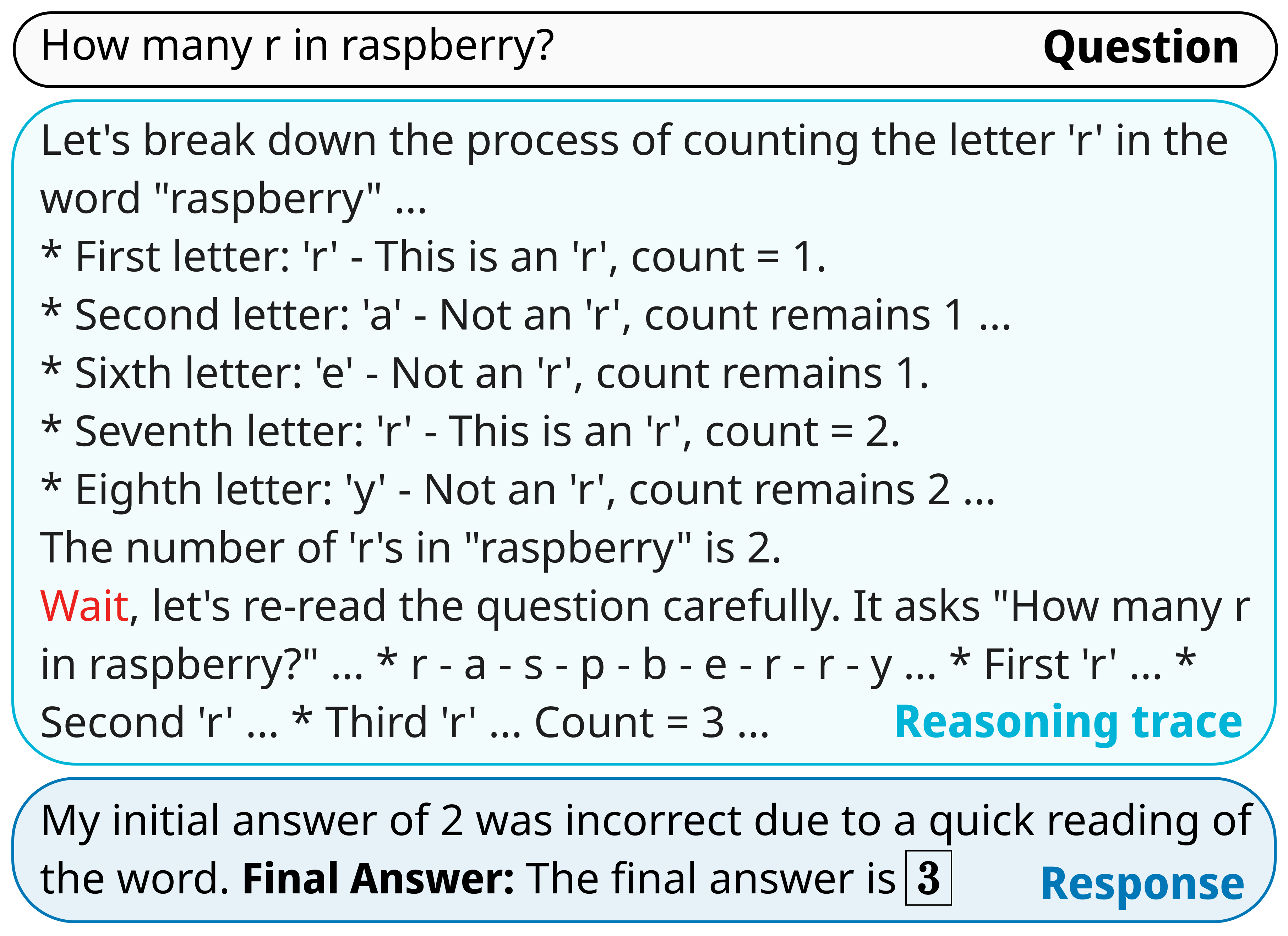
Budget forcing changes the stopping behavior of a trained reasoning model. The retained raspberry example illustrates one successful correction after an inserted continuation cue.
Original figure
Figure 3: Budget forcing with s1-32B. The model tries to stop after “…is 2.”, but we suppress the end-of-thinking token delimiter instead appending “Wait” leading s1-32B to self-correct its answer.

3.1 Method

Sequential scaling extends a dependent reasoning trajectory; parallel scaling generates independent candidates and aggregates them. The paper focuses on sequential budget control, while later experiments combine it with parallel search.

Budget forcing

To impose a maximum thinking budget, append the answer delimiter, optionally followed by “Final Answer:”, when the limit is reached. To extend thinking, suppress the delimiter when the model tries to stop and insert “Wait”, or another tested continuation string. Final-answer tokens are additional to the thinking budget.

The intervention controls an output format and token count. It neither verifies the reasoning nor guarantees that the next continuation will improve the answer. Excessive continuation can produce repetitive loops.

Baselines

Baselines ask for a token limit, a step limit, or a qualitatively short/long response. Rejection sampling repeatedly generates until a response meets a length constraint. It is an oracle-like way to condition on length, whose discarded attempts incur substantial extra compute.

3.2 Metrics

The retained equations define three summaries over tested budgets: compliance with the requested range, average pairwise accuracy-versus-token slope, and the best observed accuracy. The slope averages all pairs of evaluation points, rather than only adjacent segments, so the tested budgets affect it.

Token counts are a compute proxy rather than a full latency or cost measurement. The later analyses sometimes exclude answer tokens, step delimiters, rejected attempts, or reward-model work. The source’s claim that any monotonically increasing curve reaches 100% is not implied by monotonicity: a curve can approach a lower ceiling.

Equations 1–3
Control=1|𝒜|​∑a∈𝒜𝕀⁡(amin≤a≤amax)\displaystyle\text{Control}=\frac{1}{|\mathcal{A}|}\sum_{a\in\mathcal{A}}\mathbb{I}(a_{\text{min}}\leq a\leq a_{\text{max}}) (1)
Scaling=1(|𝒜|2)​∑a,b∈𝒜b>af⁡(b)−f⁡(a)b−a\displaystyle\text{Scaling}=\frac{1}{\binom{|\mathcal{A}|}{2}}\sum_{\begin{subarray}{c}a,b\in\mathcal{A}\\ b>a\end{subarray}}\frac{f(b)-f(a)}{b-a} (2)
Performance =maxa∈𝒜⁡f⁡(a)\displaystyle=\max_{a\in\mathcal{A}}f(a) (3)
Refer to caption
(a) Sequential scaling via budget forcing
Refer to caption
(b) Parallel scaling via majority voting
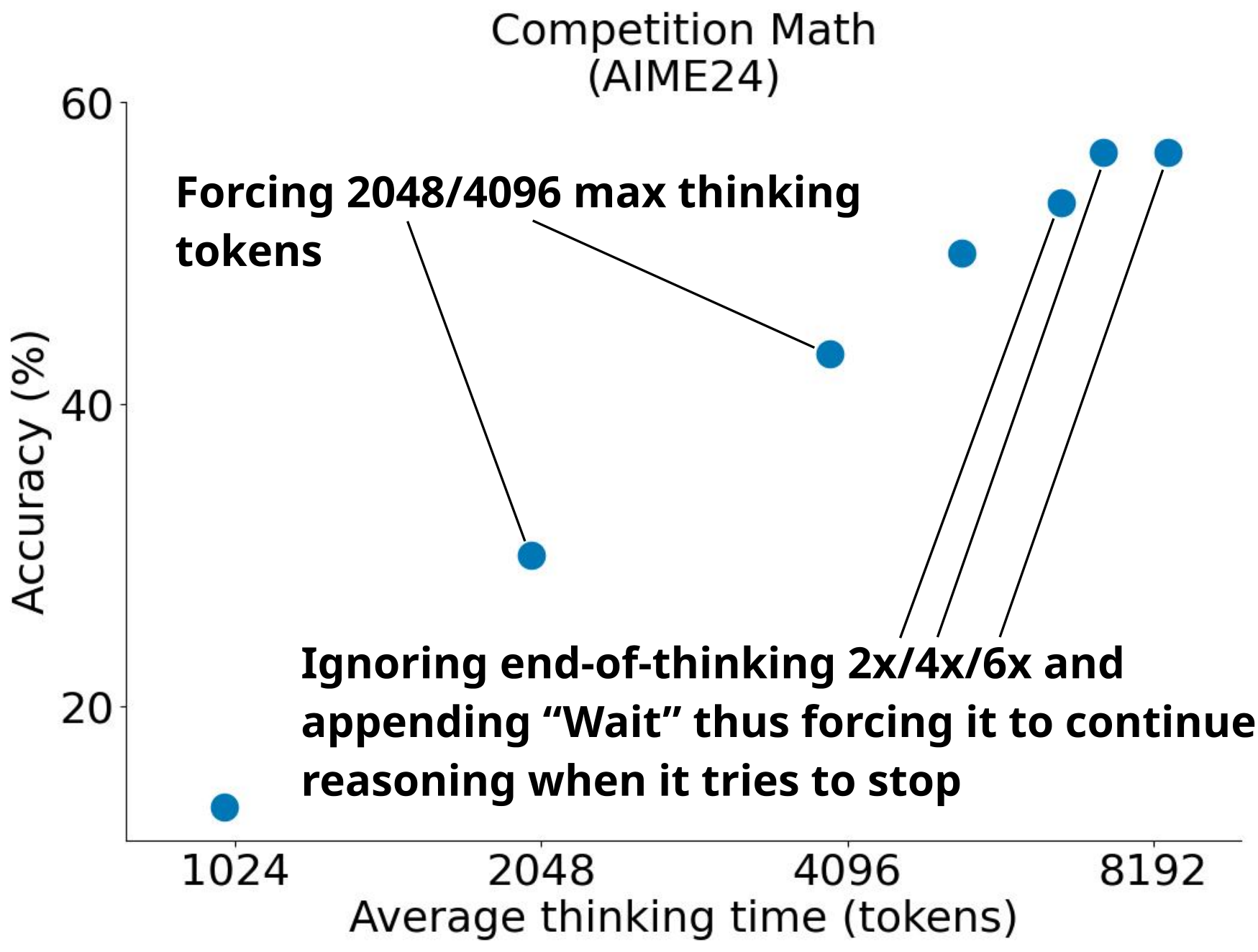
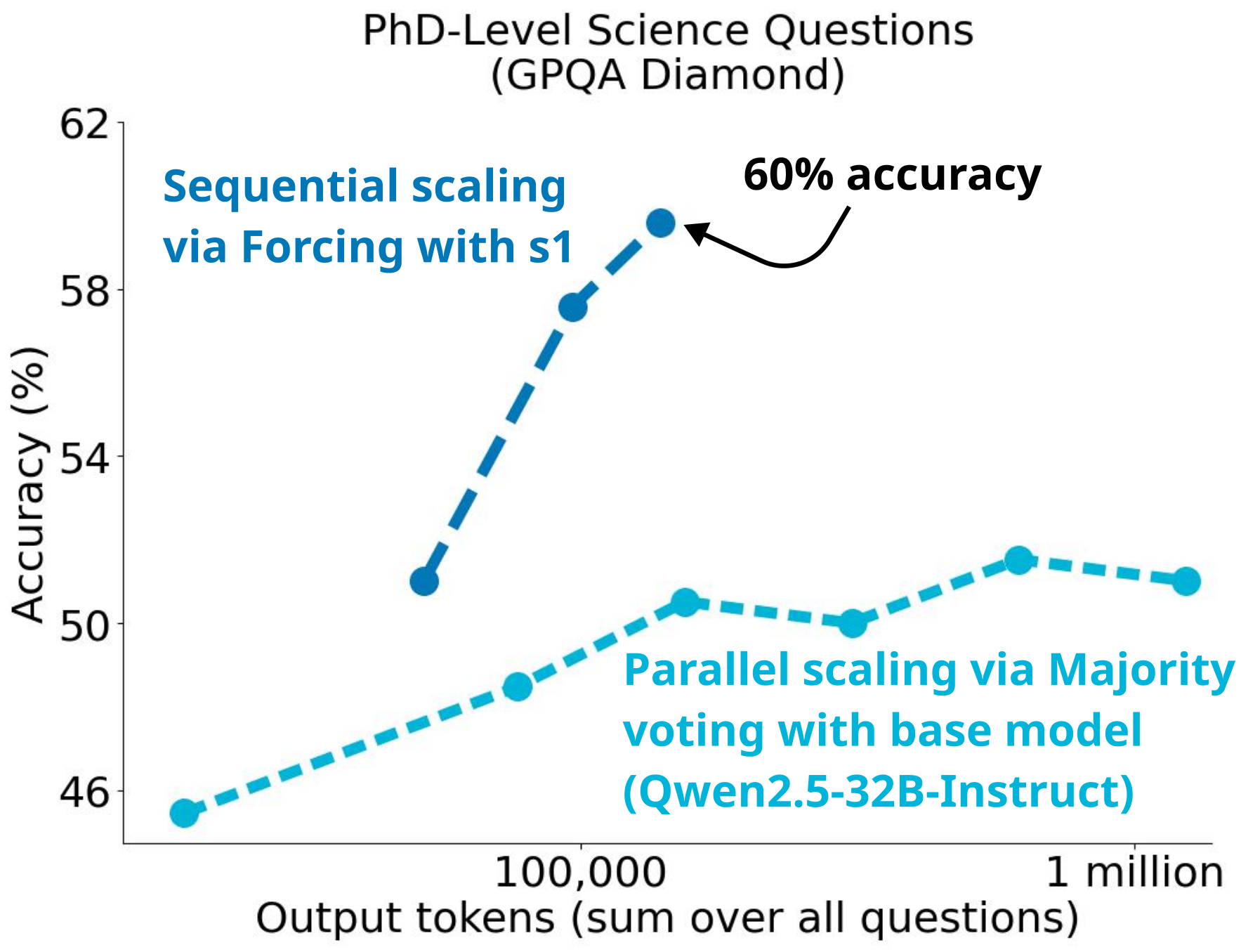
Figure 4: Sequential and parallel test-time scaling. (a): Budget forcing shows clear scaling trends and extrapolates to some extent. For the three rightmost dots, we prevent the model from stopping its thinking 2/4/6 times, each time appending “Wait” to its current reasoning trace. (b): For Qwen2.5-32B-Instruct we perform 64 evaluations for each sample with a temperature of 1 and visualize the performance when majority voting across 2, 4, 8, 16, 32, and 64 of these.

4 Results

Experiments measure the fine-tuned model, budget interventions, and comparisons with contemporary reported baselines.

4.1 Setup

The main setup uses a 32-billion-parameter instruction-tuned base model and three math/science benchmarks.

Training

Supervised training starts from Qwen2.5-32B-Instruct and predicts the teacher reasoning and answer tokens. The final s1 run takes 26 minutes on sixteen H100 GPUs, approximately seven GPU-hours. This excludes pretraining, teacher inference, data grading, and development.

Evaluation

AIME24 has thirty competition-math problems, MATH500 has five hundred, and GPQA Diamond has 198 science questions. AIME diagrams are supplied as Asymptote code because the model is text-only. Unless specified otherwise, evaluation uses greedy decoding and accuracy/pass@1. AIME’s small sample means each additional correct answer changes accuracy by about 3.3 points.

Other models

The main table combines the authors’ Qwen, s1, and Gemini evaluations with scores from other model reports. Gemini’s AIME questions were entered manually through its web interface after API recitation errors; its other benchmark entries are left unavailable. These comparisons are not uniformly rerun under one protocol.

Table 1: s1-32B is a strong open reasoning model. We evaluate s1-32B, Qwen, and Gemini (some entries are unknown (N.A.), see §4). Other results are from the respective reports (Qwen et al., 2024; Team, 2024; OpenAI, 2024; DeepSeek-AI et al., 2025; Labs, 2025; Team, 2025). # ex. = number examples used for reasoning finetuning; BF = budget forcing. See §A for our better s1.1 model.
Model # ex. AIME 2024 MATH 500 GPQA Diamond
API only
o1-preview N.A. 44.6 85.5 73.3
o1-mini N.A. 70.0 90.0 60.0
o1 N.A. 74.4 94.8 77.3
Gemini 2.0 N.A. 60.0 N.A. N.A.
Flash Think.
Open Weights
Qwen2.5- N.A. 26.7 84.0 49.0
32B-Instruct
QwQ-32B N.A. 50.0 90.6 54.5
r1 ≫\gg800K 79.8 97.3 71.5
r1-distill 800K 72.6 94.3 62.1
Open Weights and Open Data
Sky-T1 17K 43.3 82.4 56.8
Bespoke-32B 17K 63.3 93.0 58.1
s1 w/o BF 1K 50.0 92.6 56.6
s1-32B 1K 56.7 93.0 59.6

4.2 Performance

The strongest conclusions are the within-model improvements and the effectiveness of the selected fine-tuning set; cross-model sample counts describe only an additional training stage.

Test-time scaling

Budget forcing yields increasing accuracy across the tested range, then AIME performance plateaus when the model is forced to continue several times. The model can loop instead of making progress.

A GPQA plot compares sequentially scaled s1 with majority voting on the unmodified base model. That contrast changes both training and inference strategy, so it does not isolate a universal advantage of sequential over parallel computation. Later experiments show that parallel methods can complement sequential scaling.

Sample-efficiency

Without budget forcing, s1 scores 50.0 on AIME24, 92.6 on MATH500, and 56.6 on GPQA Diamond; the main budget-forced row reports 56.7, 93.0, and 59.6. Against the reported o1-preview AIME score of 44.6, 56.7 is a 12.1-point gain, about 27% relative improvement—not a 27-point gain.

The model uses far fewer final fine-tuning examples than several compared distilled models, but has inherited extensive pretraining and consumes a larger teacher/filtering pool. Stronger models in the table remain ahead on several tasks. The retained outputs illustrate correct examples, not an exhaustive accounting of errors.

Alice and Bob play the following game. A stack of nn tokens lies before them. The players take turns with Alice going first. On each turn, the player removes either 11 token or 44 tokens from the stack. Whoever removes the last token wins. Find the number of positive integers nn less than or equal to 20242024 for which there exists a strategy for Bob that guarantees that Bob will win the game regardless of Alice’s play.
The problem asks for the number of positive integers n≤2024n\leq 2024 such that Bob has a winning strategy. This is a typical impartial game that can be analyzed using the Sprague-Grundy theorem or by directly finding the winning and losing positions. Let WW be the set of winning positions (number of tokens nn such that the player whose turn it is can force a win) and LL be the set of losing positions. […]
Let P⁡(n)P(n) be the statement ”the player whose turn it is when there are nn tokens has a winning strategy. P⁡(0)P(0) is false (the player whose turn it is and faces 00 tokens has already lost). Consider the small values of nn:
n=1n=1: The player whose turn it is can take 11 token and win. So P⁡(1)P(1) is true. 1∈W1\in W.
n=2n=2: The player whose turn it is can take 11 token, leaving 11 token for the opponent. Since 1∈W1\in W, the opponent wins. So P⁡(2)P(2) is false. 2∈L2\in L.
n=3n=3: The player whose turn it is can take 11 token, leaving 22 tokens for the opponent. Since 2∈L2\in L, the player whose turn it is wins. So P⁡(3)P(3) is true. 3∈W3\in W.[…]
We are looking for the number of positive integers n≤2024n\leq 2024 for which Bob has a winning strategy. This means that if the game starts with nn tokens, and Alice goes first, Bob can win. This happens if and only if nn is a losing position (because if n∈Ln\in L, then Alice’s first move must lead to a winning position for Bob). […]
Let’s try to find a pattern in the losing positions L={0,2,5,7,10,12,15,17,20,22,…}L=\{0,2,5,7,10,12,15,17,20,22,...\}. Differences between consecutive terms: 2,3,2,3,2,3,2,3,2,…2,3,2,3,2,3,2,3,2,... The pattern of differences is alternating 2,32,3. […]
The losing positions are of the form 5​m5m or 5​m+25m+2, where m≥0m\geq 0. We need to find the number of positive integers n≤2024n\leq 2024 that are in the set of losing positions LL. […]
Case 1: n=5​mn=5m, where m≥1m\geq 1. 1≤5​m≤20241\leq 5m\leq 2024 1/5≤m≤2024/5=404.81/5\leq m\leq 2024/5=404.8 Since mm is an integer, 1≤m≤4041\leq m\leq 404. The number of values of mm is 404404.
Case 2: n=5​m+2n=5m+2, where m≥0m\geq 0. 5​m+2≤20245m+2\leq 2024 5​m≤20225m\leq 2022 m≤2022/5=404.4m\leq 2022/5=404.4 Since mm is an integer, 0≤m≤4040\leq m\leq 404. The number of values of mm is 404−0+1=405404-0+1=405.
The total number of positive integers n≤2024n\leq 2024 that are losing positions is 404+405=809404+405=\boxed{809}.
Find the projection of aa onto b=(263)b=\begin{pmatrix}2\\ 6\\ 3\end{pmatrix} if a⋅b=8.a\cdot b=8.
The projection of vector 𝐚\mathbf{a} onto vector 𝐛\mathbf{b} is given by the formula:
Equationproj𝐛​𝐚=𝐚⋅𝐛‖𝐛‖2​𝐛\text{proj}_{\mathbf{b}}\mathbf{a}=\frac{\mathbf{a}\cdot\mathbf{b}}{\|\mathbf{b}\|^{2}}\mathbf{b}
We are given 𝐛=(263)\mathbf{b}=\begin{pmatrix}2\\ 6\\ 3\end{pmatrix} and 𝐚⋅𝐛=8.\mathbf{a}\cdot\mathbf{b}=8.
First, we need to find the magnitude squared of 𝐛\mathbf{b}, which is ‖𝐛‖2\|\mathbf{b}\|^{2}.
Equation‖𝐛‖2=𝐛⋅𝐛=22+62+32=4+36+9=49.\|\mathbf{b}\|^{2}=\mathbf{b}\cdot\mathbf{b}=2^{2}+6^{2}+3^{2}=4+36+9=49.
Now we can plug the values into the projection formula:
Equationproj𝐛​𝐚=849​𝐛\text{proj}_{\mathbf{b}}\mathbf{a}=\frac{8}{49}\mathbf{b}
Substitute the vector 𝐛\mathbf{b}:
Equationproj𝐛​𝐚=849​(263)\text{proj}_{\mathbf{b}}\mathbf{a}=\frac{8}{49}\begin{pmatrix}2\\ 6\\ 3\end{pmatrix}
Multiply the scalar by each component of the vector:
Equationproj𝐛​𝐚=(849×2849×6849×3)=(164948492449)\text{proj}_{\mathbf{b}}\mathbf{a}=\begin{pmatrix}\frac{8}{49}\times 2\\ \frac{8}{49}\times 6\\ \frac{8}{49}\times 3\end{pmatrix}=\begin{pmatrix}\frac{16}{49}\\ \frac{48}{49}\\ \frac{24}{49}\end{pmatrix}
Final Answer: The final answer is
Equation(164948492449)\boxed{\begin{pmatrix}\frac{16}{49}\\ \frac{48}{49}\\ \frac{24}{49}\end{pmatrix}}
A quantum mechanical particle of mass mm moves in two dimensions in the following potential, as a function of the polar coordinates (r,θ)(r,\theta):
EquationV⁡(r,θ)=12​k​r2+32​k​r2​cos2⁡(θ)V(r,\theta)=\frac{1}{2}kr^{2}+\frac{3}{2}kr^{2}\cos^{2}(\theta)
Find the energy spectrum. Hint: Write the potential in Cartesian coordinates.
The problem asks for the energy spectrum of a particle in a given 2D potential. The potential is given in polar coordinates (r,θ)(r,\theta):
EquationV⁡(r,θ)=12​k​r2+32​k​r2​cos2⁡(θ).V(r,\theta)=\frac{1}{2}kr^{2}+\frac{3}{2}kr^{2}\cos^{2}(\theta).
We can rewrite the potential as:
EquationV⁡(r,θ)=12​k​r2​(1+3​cos2⁡(θ)).V(r,\theta)=\frac{1}{2}kr^{2}(1+3\cos^{2}(\theta)).
The Hamiltonian for a particle in 2D is given by:
EquationH=−ℏ22​m​(∂2∂x2+∂2∂y2)+V⁡(x,y).H=-\frac{\hbar^{2}}{2m}\left(\frac{\partial^{2}}{\partial x^{2}}+\frac{\partial^{2}}{\partial y^{2}}\right)+V(x,y).
In polar coordinates (r,θ)(r,\theta), the Laplacian operator is:
Equation∇2=1r​∂∂r​(r​∂∂r)+1r2​∂2∂θ2.\nabla^{2}=\frac{1}{r}\frac{\partial}{\partial r}\left(r\frac{\partial}{\partial r}\right)+\frac{1}{r^{2}}\frac{\partial^{2}}{\partial\theta^{2}}.
So the Hamiltonian in polar coordinates is:
EquationH=−ℏ22​m​[1r​∂∂r​(r​∂∂r)+1r2​∂2∂θ2]+V⁡(r,θ).H=-\frac{\hbar^{2}}{2m}\left[\frac{1}{r}\frac{\partial}{\partial r}\left(r\frac{\partial}{\partial r}\right)+\frac{1}{r^{2}}\frac{\partial^{2}}{\partial\theta^{2}}\right]+V(r,\theta).
The time-independent Schrödinger equation is H​ψ=E​ψH\psi=E\psi. We can try to separate variables by assuming a solution of the form ψ⁡(r,θ)=R⁡(r)​Θ​(θ)\psi(r,\theta)=R(r)\Theta(\theta). […]
This confirms the energy spectrum is:
EquationE=ℏ​km​(2​nx+ny+32).E=\hbar\sqrt{\frac{k}{m}}\left(2n_{x}+n_{y}+\frac{3}{2}\right).
Final Answer: E=ℏ​km​(2​nx+ny+32)E=\hbar\sqrt{\frac{k}{m}}\left(2n_{x}+n_{y}+\frac{3}{2}\right).
Figure 5: Example model outputs. We pick a question from AIME24 (left), MATH500 (middle), and GPQA (right), where our model generates the correct answer. The black text is the prompt, the light blue text is the reasoning trace, and the blue text is the answer of s1-32B. The gray ellipsis […] indicates that the text was trimmed to fit this page, but the generated text is actually longer.

5 Ablations

Ablations separate data-selection choices from methods for allocating inference tokens.

5.1 Data Quantity, Diversity, and Difficulty

Random, domain-diverse, and longest-trace 1,000-example subsets all trail the chosen s1K set on AIME24; the longest-trace subset scores higher on GPQA. The reported paired bootstrap intervals show that several differences are uncertain, especially on the thirty-question AIME test. They do not establish uniformly significant benefits across every task.

Training on all 59K examples scores 53.3/92.8/58.1 on AIME/MATH/GPQA versus 50.0/93.0/57.6 for s1K in this ablation. It costs 394 H100 GPU-hours versus about seven for the final small run. The comparison supports efficient selection, rather than equality of the methods. This table uses an approximately 30,000-token cap and a best-guess answer for looping cases; it is not identical to the uncapped main-table setting.

Table 2: s1K data ablations. We budget force (BF) a maximum of around 30,000 thinking tokens for all scores in this table. This performs slightly better than the scores without BF (Table 1) as it allows the model to finish with a best guess when stuck in an infinite loop. We report 95% paired bootstrap confidence intervals for differences relative to the s1K model using 10,000 bootstrap samples. E.g., the interval [-13%, 20%] means that, with 95% confidence, the true difference between 59K-full and s1K is between -13% and +20%. If the entire interval is negative, e.g. [-27%, -3%], we can confidently say that the performance is worse than s1K.
Model AIME 2024 MATH 500 GPQA Diamond
1K-random 36.7 90.6 52.0
[-26.7%, -3.3%] [-4.8%, 0.0%] [-12.6%, 2.5%]
1K-diverse 26.7 91.2 54.6
[-40.0%, -10.0%] [-4.0%, 0.2%] [-10.1%, 5.1%]
1K-longest 33.3 90.4 59.6
[-36.7%, 0.0%] [-5.0%, -0.2%] [-5.1%, 10.1%]
59K-full 53.3 92.8 58.1
[-13.3%, 20.0%] [-2.6%, 2.2%] [-6.6%, 8.6%]
s1K 50.0 93.0 57.6

5.2 Test-time scaling methods

Budget forcing attains perfect control on the tested budget metric, a positive scaling slope, and the best AIME score in this comparison. Prompt-only control is less reliable, and class-conditional control’s steep slope is based on just two settings.

Table 3: Ablations on methods to scale test-time compute on AIME24. |𝒜||\mathcal{A}| refers to the number of evaluation runs used to estimate the properties; thus a higher value indicates more robustness. Bold indicates our chosen method and the best values. BF = budget forcing, TCC/SCC/CCC = token/step/class-conditional control, RS = rejection sampling.
Method Control Scaling Performance |𝒜||\mathcal{A}|
BF 100% 15 56.7 5
TCC 40% -24 40.0 5
TCC + BF 100% 13 40.0 5
SCC 60% 3 36.7 5
SCC + BF 100% 6 36.7 5
CCC 50% 25 36.7 2
RS 100% -35 40.0 5

Budget forcing

With two forced continuations, “Wait” scores 53.3/93.0/59.6 across AIME/MATH/GPQA. It improves AIME by one question over no extrapolation and ties or exceeds the alternatives, but is not uniquely best on every benchmark. Appending no string can reduce MATH and GPQA accuracy.

Token instructions are frequently ignored; step instructions permit the model to use more tokens per step. External budget enforcement makes these controls more reliable, while qualitative short/long instructions give only coarse and inconsistent changes.

Table 4: Budget forcing extrapolation ablations. We compare ignoring the end-of-thinking delimiter twice and appending none or various strings.
Model AIME 2024 MATH 500 GPQA Diamond
No extrapolation 50.0 93.0 57.6
2x without string 50.0 90.2 55.1
2x “Alternatively” 50.0 92.2 59.6
2x “Hmm” 50.0 93.0 59.6
2x “Wait” 53.3 93.0 59.6
Original figure
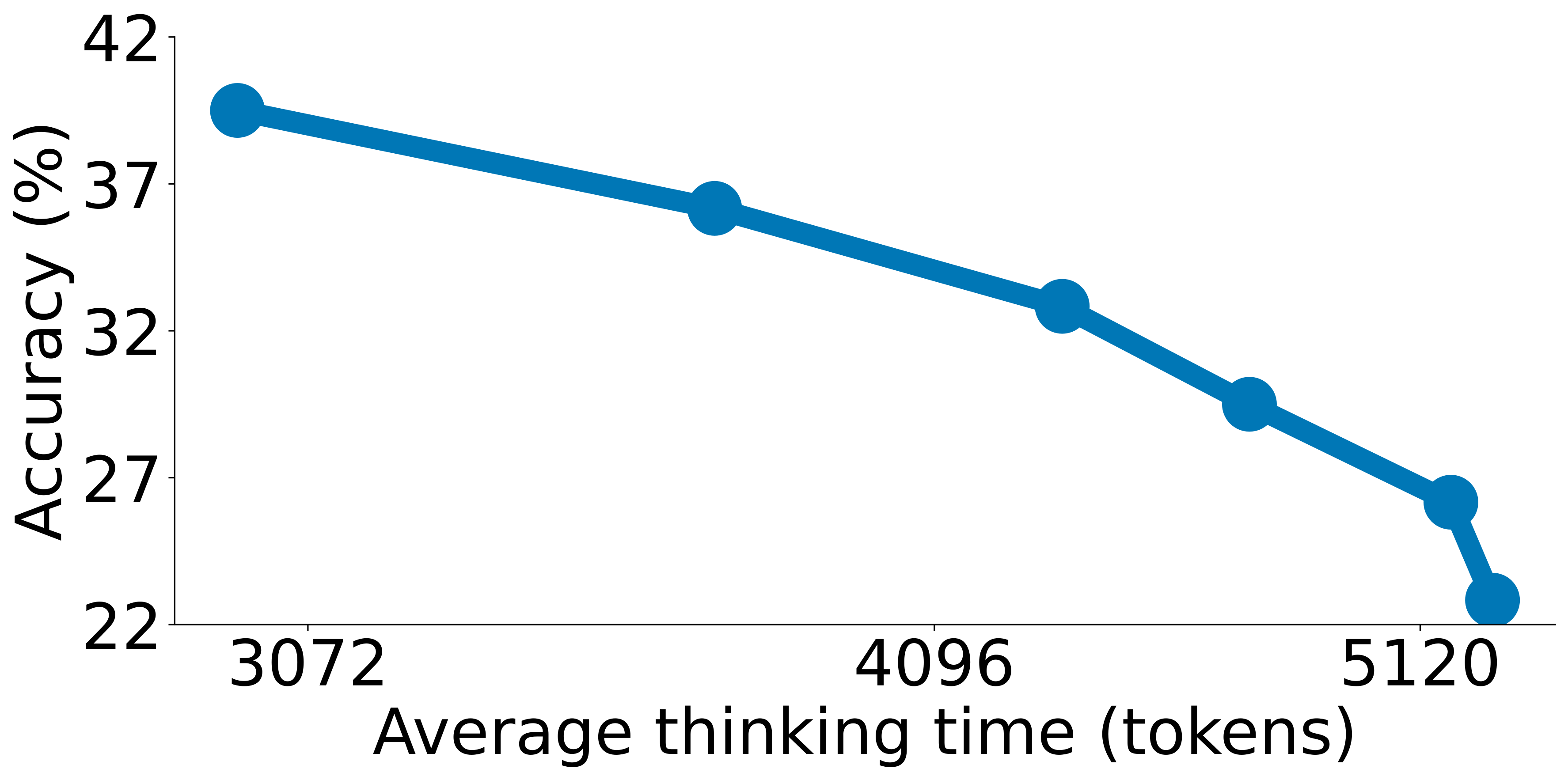
Figure 6: Rejection sampling on AIME24 with s1-32B. We sample with a temperature of 1 until all generations have less than (from left to right) 3500, 4000, 5000, 8000, and 16000 thinking tokens requiring an average of 655, 97, 8, 3, 2, and 1 tries per sample.

Rejection sampling

Conditioning sampled responses on shorter lengths yields better AIME accuracy in the tested rejection experiment. The authors hypothesize that easy, initially correct reasoning finishes early, while mistaken trajectories backtrack. This correlation does not show that forcibly shortening an arbitrary trajectory causes correctness.

The apparent short-output advantage omits discarded sampling work: the tightest conditions require hundreds of attempts per accepted response. The figure caption lists five thresholds but six attempt counts, so no exact one-to-one mapping should be inferred for all entries. The full qualitative comparison is retained in the supplement.

6 Discussion and related work

The discussion connects sample-efficient adaptation with inference search and considers limits to further extrapolation.

6.1 Sample-efficient reasoning

A small final dataset can substantially change how a pretrained model uses its existing capabilities, but this work does not determine how those capabilities were acquired.

Models

The authors relate their result to LIMA: a small supervised set may elicit abilities already present after pretraining. This is a hypothesis, not a demonstrated internal mechanism. Comparisons with DeepSeek-r1 and other contemporary systems distinguish supervised distillation from reinforcement-learning approaches without proving either universally preferable.

Benchmarks and methods

Related methods include continued math/science pretraining, synthetic data, specialized reasoning training, and prompting or search procedures. More difficult science, olympiad, coding, and general reasoning benchmarks motivate these developments, but the experiments here cover only the reported math/science tasks.

6.2 Test-time scaling

Inference scaling involves both deciding how to spend compute and assessing whether the extra work improves the selected answer.

Methods

Parallel methods use majority voting or reward-based candidate selection. Sequential methods revise earlier attempts, while tree search combines dependent steps with branching. Outcome reward models score complete answers; process reward models evaluate intermediate steps. The cited REBASE method uses process rewards to allocate search effort.

Limits to further test-time scaling

Budget forcing eventually saturates and is bounded by the model’s context window. The authors suggest varying continuation strings, sampling settings, frequency penalties, and reinforcement-learning training as possible extensions. These are future directions rather than validated remedies in this paper.
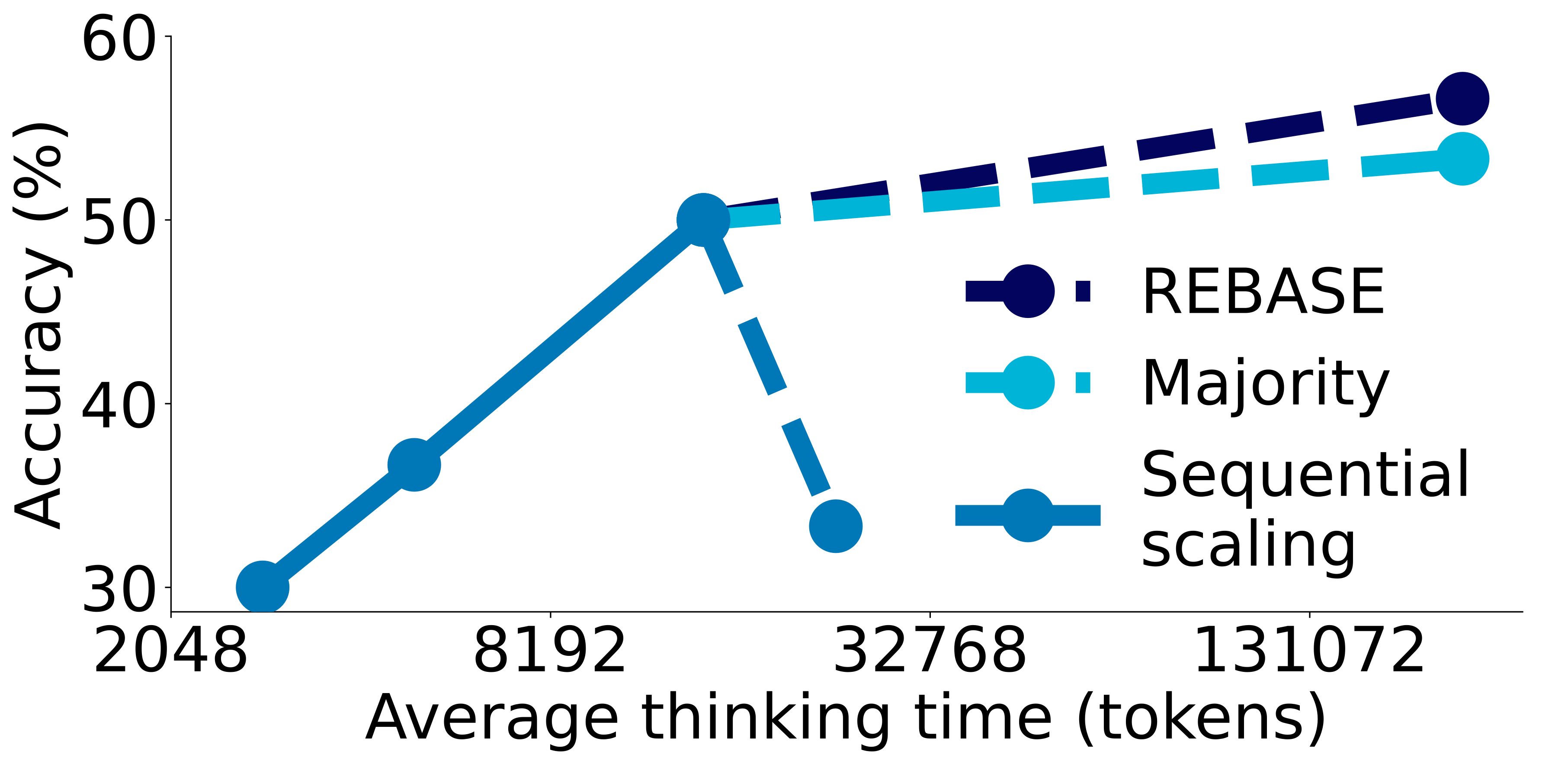
Original figure
Figure 7: Scaling further with parallel scaling methods. All metrics averaged over the 30 questions in AIME24. Average thinking tokens for REBASE do not account for the additional compute from the reward model. For sequential scaling, we prompt the model to use up to (from left to right) 32, 64, 256, and 512 steps. For REBASE and majority voting we generate 16 parallel trajectories to aggregate across.

Parallel scaling as a solution

On an earlier step-controlled model, sixteen parallel trajectories with REBASE or majority voting improve on the longest unsuccessful sequential setting. At 512 requested steps, twelve of thirty questions exceed the context window. REBASE’s plotted token count excludes the additional reward-model forward passes, so it does not represent equal total compute.

This experiment uses an earlier dataset and evaluation codebase, as the appendix states. It demonstrates a possible complementary route to more inference compute; its numbers should not be silently merged with the final s1 results.

Impact Statement

The authors frame open weights, data, and methods as a way to make reasoning research more reproducible and accessible. The impact statement discusses potential productivity and scientific benefits; it does not evaluate downstream deployment outcomes.

Acknowledgements

Acknowledgments credit DeepSeek-r1 trace generation through Bespoke Curator, Stanford’s Marlowe cluster, institutional support, and research discussions.

Appendix A s1.1

s1.1 keeps the same 1,000 questions and training procedure but regenerates the traces with DeepSeek-r1. Without forcing it scores 94.4 on MATH500, 60.6 on GPQA, 56.7 on AIME24, and 50.0 on AIME25. Two “Wait” continuations raise MATH/GPQA to 95.4/63.6 while leaving both AIME scores unchanged.

The complete updated comparison table is retained. Its r1 MATH500 entry is printed as 07.3 in both HTML and PDF, conflicting with 97.3 in the main table; the original value is preserved as a source typo. Some comparison-model AIME24 values also differ from the main table, so the rows are not a uniformly matched reevaluation. The unreported Claude-distillation experiment supplies no scores to assess.

Table 5: s1-32B is an open and sample-efficient reasoning model. We evaluate s1-32B, Qwen, and Gemini (some entries are unknown (N.A.), see §4). Other results are from the respective reports (Qwen et al., 2024; Team, 2024; OpenAI, 2024; OpenAI, 2025; DeepSeek-AI et al., 2025; Labs, 2025; Team, 2025) except for AIME 2025 (Ye et al., 2025b). # ex. = number examples used for reasoning finetuning; BF = budget forcing.
Model # Examples MATH500 GPQA AIME 2024 AIME 2025
API only
o3-mini-low N/A 95.8 70.6 56.3 42.1
o3-mini-medium N/A 97.3 76.8 75.8 70.4
o3-mini-high N/A 97.9 79.7 83.8 80.9
Open Weights
QwQ-32B N.A. 90.6 54.5 46.7 32.7
r1 ≫\gg800K 07.3 71.5 79.8 70.0
r1-distill-Llama-70B 800K 94.5 65.2 57.1 56.3
r1-distill-Qwen-14B 800K 93.9 59.1 61.7 48.0
r1-distill-Qwen-32B 800K 94.3 62.1 58.3 49.6
Open Weights and Open Data
LIMO 817 94.8 66.7 56.3 44.6
s1 w/o BF 1K 92.6 56.6 50.0 26.7
s1 with Budget Forcing “Wait” 1x 1K 92.8 59.6 53.3 30.0
s1 with Budget Forcing “Wait” 2x 1K 93.0 59.6 53.3 33.3
s1 with Budget Forcing “Wait” 4x 1K 92.2 58.6 56.7 36.7
s1.1 w/o BF 1K 94.4 60.6 56.7 50.0
s1.1 with Budget Forcing “Wait” 1x 1K 95.4 62.6 56.7 50.0
s1.1 with Budget Forcing “Wait” 2x 1K 95.4 63.6 56.7 50.0

Appendix B Evaluation determinism

Greedy decoding with a fixed seed is not always deterministic in the authors’ vLLM setup. Batch size, continuation calls, tensor parallelism, and numerical precision can change one token after a long shared prefix, eventually changing the answer. Final evaluations generally use full precision to reduce this sensitivity, without claiming complete determinism.

Appendix C s1K details

The supplement retains the full domain/source inventories, grading prompt, selection algorithm, and decontamination description.

C.1 s1K summary

The final set contains about 4.7 million tokens under the Qwen tokenizer. Geometry, number theory, and combinatorics are the largest domains. The table’s total-domain label is inconsistent with the prose and its own listed-plus-remaining count; all original rows and values remain visible.

Table 6: Summary of our dataset s1K. Token count measured by the Qwen-2.5 tokenizer. We prompt Claude to produce keywords given several questions from the domain.
Domain
#questions Total token count Keywords
Geometry
109 560.2K Area, Triangle, Distance
Number theory
98 522.5K Sequences, Divisibility
Combinatorics
75 384.7K Permutations, Counting
Real functions
43 234.8K Trigonometry, Calculus
Biology
41 120.9K Organic reactions
Complex functions
32 170.2K Complex roots
Quantum theory
32 127.9K Particles, Wave functions
Field theory
28 150.1K Polynomials, Roots
Calculus of variations
28 155.5K Optimization, Control
Difference equations
24 132.5K Recurrence, Recursion
Electromagnetic theory
23 95.8K Optics, Waves, Diffraction
Group theory
22 100.0K Groups, Automorphisms
Linear algebra
22 128.3K Matrices, Determinants
Probability theory
20 114.6K Random walk, Expectation
Algebraic systems
19 109.9K Functional equations
Mechanics
19 103.6K Forces, Motion, Energy
Thermodynamics
19 74.2K Heat engines, Entropy
Differential equations
18 89.6K Substitution, Existence
Computer science
18 34.2K Complexity theory, Algorithms
Numerical analysis
18 76.5K Error analysis, Stability
Calculus
17 96.3K Convergence, Summation
Algebraic structures
17 90.4K Inequalities, Sets
Astronomy
16 37.7K Stellar populations, Orbits
Remaining 27 domains
242 982.2K Domains with ≤\leq 16 questions
All domains (51)
1000 4.7M s1K

C.2 Dataset composition for full 59K questions

The sixteen-source table gives all 59,029 candidate counts and mean thinking lengths. Besides evaluation AIME24 questions, the authors exclude 2022–2023 AIME questions used during development. Source overlap screening does not establish absence of related content in the pretrained or teacher models.

Table 7: Composition of full 59K questions. Thinking and response lengths are measured in tokens using the Qwen2.5-32B-Instruct tokenizer (Qwen et al., 2024). In addition to excluding our evaluation benchmark, AIME24, we also exclude AIME questions from 2022-2023 as we use these 90 questions during our development stage of s1-32B.
Source
Description
#Samples
Avg. thinking length
NuminaMATH (LI et al., 2024)
Math problems from online websites
30660
4.1K
Math problems from competitions
11999
2.9K
OlympicArena (Huang et al., 2024a)
Astronomy, Biology, Chemistry, Computer Science, Geography, Math, and Physics olympiad questions
4250
3.2K
OmniMath (Gao et al., 2024a)
Math problems from competitions
4238
4.4K
English, Law, Logic and Math problems from the SAT, LSAT and other exams
2385
1.2K
xword
Crossword puzzles
999
0.7K
OlympiadBench (He et al., 2024)
Math and Physics olympiad questions
896
3.9K
AIME (1983-2021)
American Invitational Mathematics Examination
890
4.7K
TheoremQA (Chen et al., 2023)
Computer Science, Finance, Math, and Physics university-level questions relating to theorems
747
2.1K
Code problems from the USA Computing Olympiad
519
3.6K
Chemistry, Math, and Physics problems used in the university entrance examination of the Indian Institute of Technology
515
2.9K
PhD-Level Science Questions
348
2.9K
Biology, Chemistry, and Physics problems from various sources
227
0.7K
s1-prob
Stanford statistics qualifying exams
182
4.0K
LiveCodeBench (Jain et al., 2024)
Code problems from coding websites (LeetCode, AtCoder, and CodeForces)
151
3.5K
s1-teasers
Math brain-teasers crawled from the Internet
23
4.1K
All 59K questions
Composite of the above datasets with reasoning traces and solutions
59029
3.6K

C.3 s1K grading prompt

Claude 3.5 grades candidate attempts against reference solutions during selection. Claude 3.7 grades the final set’s correctness statistics. The exact grading prompt is preserved, including its request for a final Yes/No judgment. Automated grading is part of the selection process, not an independent proof that a trace is sound.

You are an AI assistant for grading a science problem. The user will provide you with the question itself, an attempt made by a student and the correct answer to the problem. Your job is to judge whether the attempt is correct by comparing it with the correct answer. If the expected solution concludes with a number or choice, there should be no ambiguity. If the expected solution involves going through the entire reasoning process, you should judge the attempt based on whether the reasoning process is correct with correct answer if helpful.
The user will provide the attempt and the correct answer in the following format:
# Problem
{problem}
## Attempt
{attempt}
## Correct answer
{solution}
Explain your reasoning, and end your response on a new line with only ”Yes” or ”No” (without quotes).
Figure 8: Grading prompt.

C.4 s1K diversity selection

The two-stage algorithm seeds correct AIME/GPQA examples and selected long correct MATH examples, then samples domains uniformly and questions with exponentially decaying rank weights favoring longer traces. Chosen questions are removed from their domain pool and exhausted domains are removed. The original algorithm is retained, including its “MATH500” comment, while the prose states that evaluation questions were excluded.

Algorithm 1 Two-stage sampling for s1K
1:  Input: 𝒬\mathcal{Q} := Set of 24,496 questions with features
2:  Output: 𝒮\mathcal{S} := Set of 1,000 selected questions
3:  𝒮←∅\mathcal{S}\leftarrow\emptyset Initialize the output set (only tracks unique elements)
4:  for q∈𝒬q\in\mathcal{Q} do
5:   if IsGeminiCorrect(qq) and (IsAIME(qq) or IsGPQA(qq)) then
6:    𝒮←𝒮∪{q}\mathcal{S}\leftarrow\mathcal{S}\cup\{q\}
7:    Select all correct AIME/GPQA solutions
8:   else if IsGeminiCorrect(qq) and IsMATH(qq) and ThinkingLength(qq) > 5600 then
9:    𝒮←𝒮∪{q}\mathcal{S}\leftarrow\mathcal{S}\cup\{q\}
10:    Select correct MATH500 solutions with long chains
11:   end if
12:  end for
13:  𝒟←\mathcal{D}\leftarrow All available domains
14:  Initialize domain pool
15:  while |𝒮|<1000|\mathcal{S}|<1000 do
16:   d←d\leftarrow RandomChoice(𝒟\mathcal{D})
17:   Randomly select a domain
18:   Qd←Q_{d}\leftarrow Questions in domain dd
19:   Get questions from this domain
20:   ranks ←\leftarrow RankByThinkingLength(QdQ_{d})
21:   Rank by thinking length
22:   weights ←2−ranks\leftarrow 2^{-\text{ranks}}
23:   Apply power-law weighting
24:   q←q\leftarrow WeightedSample(QdQ_{d}, weights)
25:   Sample favoring longer chains
26:   𝒮←𝒮∪{q}\mathcal{S}\leftarrow\mathcal{S}\cup\{q\}
27:   Add selected question
28:   Qd←Qd∖{q}Q_{d}\leftarrow Q_{d}\setminus\{q\}
29:   if Qd=∅Q_{d}=\emptyset then
30:    𝒟←𝒟∖{d}\mathcal{D}\leftarrow\mathcal{D}\setminus\{d\}
31:    Remove exhausted domains
32:   end if
33:  end while

C.5 Decontamination

Selected examples are screened for eight-gram overlap with MATH500, GPQA Diamond, and AIME24, and overlapping questions are removed. This lexical check addresses direct dataset overlap; it cannot rule out paraphrases or prior model exposure.

Appendix D Training details

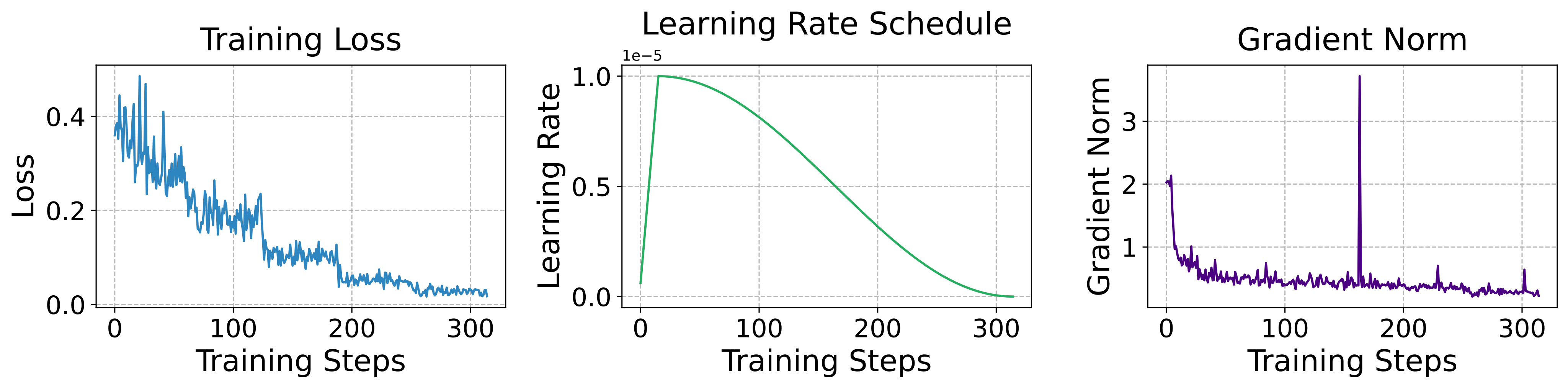
Training separates question, thinking, and answer with explicit token delimiters. The loss covers reasoning and answer tokens, not the question. Five epochs with batch size sixteen give 315 gradient steps in bfloat16. AdamW uses learning rate 10⁻⁵, β₁=0.9, β₂=0.95, and weight decay 10⁻⁴, with sixteen warmup steps and cosine decay over the remaining 299.

The sequence limit is chosen to retain complete examples. The training-dynamics figure preserves loss, learning rate, and gradient norm. The reported 26-minute run measures this final fine-tuning stage alone.
Original figure
Figure 9: Training dynamics of s1-32B on s1K.

D.1 Training Ablations: Sequence length

A 4,096-token training limit cuts off 74% of examples, while 32,768 cuts off none in the compared data. The longer-limit model generates shorter inference traces and scores better on all three benchmarks: AIME rises from 30% to 50%, while average thinking tokens fall from 20,721 to 6,984.

The proposed explanation is that complete examples provide more supervision for transitioning into an answer. That is consistent with the ablation, but the experiment does not directly isolate the mechanism or make all reported benchmark runs numerically interchangeable.

Table 8: Training sequence length ablation. We report “accuracy / average thinking tokens per sample”; the higher the accuracy and the fewer the thinking tokens (inference cost) the better.
Model A
Model B
Training sequence length
4096
32768
% training samples cutoff
74%
0%
30.0% / 20721
50.0% / 6984
90.0% / 5324
91.0% / 3268
52.5% / 6841
53.0% / 3568

D.2 Training Samples

Three complete training examples cover alternating conditional-expectation limits, conditional coin-flip counts, and an astronomy temperature problem. Each retains the question, reference solution, generated reasoning, and final response, with their original color distinctions. These are examples of the training material, including backtracking and erroneous intermediate steps; they are not newly verified mathematical proofs.

Table 9: s1K sample stemming from s1-prob. The black text is the question and the yellow text is the solution. Based solely on the question we generate the light blue reasoning trace and blue response with Gemini, which we use for training.
You are given integrable random variables X,Y0X,Y_{0} and Z0Z_{0} on the same probability space (Ω,ℱ,ℙ)(\Omega,\mathcal{F},\mathbb{P}), and two σ\sigma-algebras 𝒜⊂ℱ,ℬ⊂ℱ.\mathcal{A}\subset\mathcal{F},\mathcal{B}\subset\mathcal{F}. For k=1,2,…,k=1,2,\ldots,, let
EquationYk:=𝔼⁡[X|σ⁡(𝒜,Z0,…,Zk−1)],Zk:=𝔼⁡[X|σ⁡(ℬ,Y0,…,Yk−1)].Y_{k}:=\mathbb{E}[X|\sigma(\mathcal{A},Z_{0},\ldots,Z_{k-1})],\quad Z_{k}:=\mathbb{E}[X|\sigma(\mathcal{B},Y_{0},\ldots,Y_{k-1})].
(a) Show that there exist integrable random variables Y∞Y_{\infty} and Z∞Z_{\infty} such that as n→∞n\to\infty both 𝔼⁡[|Yn−Y∞|]→0\mathbb{E}[|Y_{n}-Y_{\infty}|]\to 0 and 𝔼⁡[|Zn−Z∞|]→0\mathbb{E}[|Z_{n}-Z_{\infty}|]\to 0. (b) Prove that almost surely Y∞=Z∞.Y_{\infty}=Z_{\infty}.
1.
Introduce the notations, ℱn:=σ⁡(𝒜,Z0,…,Zn−1)\mathcal{F}_{n}:=\sigma(\mathcal{A},Z_{0},\ldots,Z_{n-1}) and 𝒢n:=σ⁡(ℬ,Y0,…,Yn−1)\mathcal{G}_{n}:=\sigma(\mathcal{B},Y_{0},\ldots,Y_{n-1}), for all n≥1n\geq 1 and ℱ0:=𝒜\mathcal{F}_{0}:=\mathcal{A}, 𝒢0:=ℬ\mathcal{G}_{0}:=\mathcal{B}. Clearly, both are filtrations and by definition, Yn=𝔼[X|ℱn]Y_{n}=\mathbb{E}\left[X\rvert\mathcal{F}_{n}\right] and Zn=𝔼[X|𝒢n]Z_{n}=\mathbb{E}\left[X\rvert\mathcal{G}_{n}\right], for all n≥0n\geq 0. Thus {Yn}n≥0\left\{Y_{n}\right\}_{n\geq 0} (or {Zn}n≥0\left\{Z_{n}\right\}_{n\geq 0} ) is a Doob’s Martingale with respect to filtration {ℱn}n≥0\left\{\mathcal{F}_{n}\right\}_{n\geq 0} (or {𝒢n}n≥0\left\{\mathcal{G}_{n}\right\}_{n\geq 0}) and hence is U.I., XX being integrable. Now apply the fact that a Martingale is U.I. if and only if it converges in L1L^{1} and conclude.
2.
We provide two different proofs.
1.
Observe the following identity which follows from Tower Property.
Equation𝔼[Yn|𝒢n]=𝔼[𝔼[X|ℱn]|𝒢n]=𝔼[𝔼[X|𝒢n]|ℱn]=𝔼[Zn|ℱn].{}\mathbb{E}\left[Y_{n}\rvert\mathcal{G}_{n}\right]=\mathbb{E}\left[\mathbb{E}\left[X\rvert\mathcal{F}_{n}\right]\rvert\mathcal{G}_{n}\right]=\mathbb{E}\left[\mathbb{E}\left[X\rvert\mathcal{G}_{n}\right]\rvert\mathcal{F}_{n}\right]=\mathbb{E}\left[Z_{n}\rvert\mathcal{F}_{n}\right].
(4)
Note that 𝔼|𝔼[Yn|𝒢n]−𝔼[Y∞|𝒢n]|≤𝔼|Yn−Y∞|=o(1)\mathbb{E}\rvert\mathbb{E}\left[Y_{n}\rvert\mathcal{G}_{n}\right]-\mathbb{E}\left[Y_{\infty}\rvert\mathcal{G}_{n}\right]\rvert\leq\mathbb{E}|Y_{n}-Y_{\infty}|=o(1) and by Levy’s Upward Theorem, 𝔼[Y∞|𝒢n]⟶L1𝔼[Y∞|𝒢∞]\mathbb{E}\left[Y_{\infty}\rvert\mathcal{G}_{n}\right]\stackrel{{\scriptstyle L^{1}}}{{\longrightarrow}}\mathbb{E}\left[Y_{\infty}\rvert\mathcal{G}_{\infty}\right], where 𝒢∞=σ(∪n≥0𝒢n)=σ(ℬ,Y0,Y1…).\mathcal{G}_{\infty}=\sigma\left(\cup_{n\geq 0}\mathcal{G}_{n}\right)=\sigma(\mathcal{B},Y_{0},Y_{1}\ldots). It is evident that Y∞∈m​𝒢∞Y_{\infty}\in m\mathcal{G}_{\infty} (since it is almost sure limit of Yn∈m​𝒢nY_{n}\in m\mathcal{G}_{n}) and hence 𝔼[Y∞|𝒢∞]=Y∞\mathbb{E}\left[Y_{\infty}\rvert\mathcal{G}_{\infty}\right]=Y_{\infty} almost surely. Combining the above observations we conclude that 𝔼[Yn|𝒢n]⟶L1Y∞.\mathbb{E}\left[Y_{n}\rvert\mathcal{G}_{n}\right]\stackrel{{\scriptstyle L^{1}}}{{\longrightarrow}}Y_{\infty}. Similarly, 𝔼[Zn|ℱn]⟶L1Z∞.\mathbb{E}\left[Z_{n}\rvert\mathcal{F}_{n}\right]\stackrel{{\scriptstyle L^{1}}}{{\longrightarrow}}Z_{\infty}. Now invoke Equation (9), to conclude that Y∞=Z∞Y_{\infty}=Z_{\infty} almost surely.
2.
Since XX is integrable, we have by Levy’s Upward Theorem, Y∞=limn→∞Yn=limn→∞𝔼[X|ℱn]=𝔼[X|ℱ∞].Y_{\infty}=\lim_{n\to\infty}Y_{n}=\lim_{n\to\infty}\mathbb{E}\left[X\rvert\mathcal{F}_{n}\right]=\mathbb{E}\left[X\rvert\mathcal{F}_{\infty}\right]. Similarly, Z∞=𝔼[X|𝒢∞].Z_{\infty}=\mathbb{E}\left[X\rvert\mathcal{G}_{\infty}\right]. On the otherhand, in first proof we have observed that Y∞∈m​𝒢∞Y_{\infty}\in m\mathcal{G}_{\infty} and hence Y∞∈m​𝒢∞∩m​ℱ∞=m⁡(𝒢∞∩ℱ∞)Y_{\infty}\in m\mathcal{G}_{\infty}\cap m\mathcal{F}_{\infty}=m\left(\mathcal{G}_{\infty}\cap\mathcal{F}_{\infty}\right). This yields the following.
EquationY∞=𝔼[Y∞|𝒢∞∩ℱ∞]=𝔼[𝔼[X|ℱ∞]|𝒢∞∩ℱ∞]=𝔼[X|𝒢∞∩ℱ∞].Y_{\infty}=\mathbb{E}\left[Y_{\infty}\rvert\mathcal{G}_{\infty}\cap\mathcal{F}_{\infty}\right]=\mathbb{E}\left[\mathbb{E}\left[X\rvert\mathcal{F}_{\infty}\right]\rvert\mathcal{G}_{\infty}\cap\mathcal{F}_{\infty}\right]=\mathbb{E}\left[X\rvert\mathcal{G}_{\infty}\cap\mathcal{F}_{\infty}\right].
Similarly, Z∞=𝔼[X|𝒢∞∩ℱ∞].Z_{\infty}=\mathbb{E}\left[X\rvert\mathcal{G}_{\infty}\cap\mathcal{F}_{\infty}\right]. This proves that Y∞=Z∞Y_{\infty}=Z_{\infty} almost surely.
Let’s analyze the problem. We are given two sequences of random variables YkY_{k} and ZkZ_{k} defined by conditional expectations. We need to show that these sequences converge in L1L^{1} and that their limits are equal almost surely.
Part (a): Convergence in L1L^{1}.
The sigma-algebras involved are increasing:
ℱk=σ⁡(𝒜,Z0,…,Zk−1)\mathcal{F}_{k}=\sigma(\mathcal{A},Z_{0},\ldots,Z_{k-1})
𝒢k=σ⁡(ℬ,Y0,…,Yk−1)\mathcal{G}_{k}=\sigma(\mathcal{B},Y_{0},\ldots,Y_{k-1})
For the YkY_{k} sequence:
Y1=𝔼⁡[X|σ⁡(𝒜)]Y_{1}=\mathbb{E}[X|\sigma(\mathcal{A})]
Y2=𝔼⁡[X|σ⁡(𝒜,Z0)]Y_{2}=\mathbb{E}[X|\sigma(\mathcal{A},Z_{0})]
Y3=𝔼⁡[X|σ⁡(𝒜,Z0,Z1)]Y_{3}=\mathbb{E}[X|\sigma(\mathcal{A},Z_{0},Z_{1})]
…
The sequence of sigma-algebras σ⁡(𝒜,Z0,…,Zk−1)\sigma(\mathcal{A},Z_{0},\ldots,Z_{k-1}) is increasing. By the Martingale Convergence Theorem (for conditional expectations), since XX is integrable, the sequence YkY_{k} converges almost surely and in L1L^{1} to 𝔼⁡[X|σ⁡(𝒜,Z0,Z1,…)]\mathbb{E}[X|\sigma(\mathcal{A},Z_{0},Z_{1},\ldots)]. Let Y∞=𝔼⁡[X|σ⁡(𝒜,Z0,Z1,…)]Y_{\infty}=\mathbb{E}[X|\sigma(\mathcal{A},Z_{0},Z_{1},\ldots)].
Similarly, for the ZkZ_{k} sequence:
Z1=𝔼⁡[X|σ⁡(ℬ)]Z_{1}=\mathbb{E}[X|\sigma(\mathcal{B})]
Z2=𝔼⁡[X|σ⁡(ℬ,Y0)]Z_{2}=\mathbb{E}[X|\sigma(\mathcal{B},Y_{0})]
Z3=𝔼⁡[X|σ⁡(ℬ,Y0,Y1)]Z_{3}=\mathbb{E}[X|\sigma(\mathcal{B},Y_{0},Y_{1})]
…
The sequence of sigma-algebras σ⁡(ℬ,Y0,…,Yk−1)\sigma(\mathcal{B},Y_{0},\ldots,Y_{k-1}) is increasing. By the Martingale Convergence Theorem, the sequence ZkZ_{k} converges almost surely and in L1L^{1} to 𝔼⁡[X|σ⁡(ℬ,Y0,Y1,…)]\mathbb{E}[X|\sigma(\mathcal{B},Y_{0},Y_{1},\ldots)]. Let Z∞=𝔼⁡[X|σ⁡(ℬ,Y0,Y1,…)]Z_{\infty}=\mathbb{E}[X|\sigma(\mathcal{B},Y_{0},Y_{1},\ldots)].
Part (b): Prove that almost surely Y∞=Z∞Y_{\infty}=Z_{\infty}.
We have Y∞=𝔼⁡[X|σ⁡(𝒜,Z0,Z1,…)]Y_{\infty}=\mathbb{E}[X|\sigma(\mathcal{A},Z_{0},Z_{1},\ldots)] and Z∞=𝔼⁡[X|σ⁡(ℬ,Y0,Y1,…)]Z_{\infty}=\mathbb{E}[X|\sigma(\mathcal{B},Y_{0},Y_{1},\ldots)].
Let 𝒴∞=σ⁡(𝒜,Z0,Z1,…)\mathcal{Y}_{\infty}=\sigma(\mathcal{A},Z_{0},Z_{1},\ldots) and 𝒵∞=σ⁡(ℬ,Y0,Y1,…)\mathcal{Z}_{\infty}=\sigma(\mathcal{B},Y_{0},Y_{1},\ldots).
Then Y∞=𝔼⁡[X|𝒴∞]Y_{\infty}=\mathbb{E}[X|\mathcal{Y}_{\infty}] and Z∞=𝔼⁡[X|𝒵∞]Z_{\infty}=\mathbb{E}[X|\mathcal{Z}_{\infty}].
Consider Y1=𝔼⁡[X|𝒜]Y_{1}=\mathbb{E}[X|\mathcal{A}]. Z1=𝔼⁡[X|ℬ]Z_{1}=\mathbb{E}[X|\mathcal{B}].
Y2=𝔼⁡[X|σ⁡(𝒜,Z0)]Y_{2}=\mathbb{E}[X|\sigma(\mathcal{A},Z_{0})]. Since Z0=𝔼⁡[X|ℬ]Z_{0}=\mathbb{E}[X|\mathcal{B}], σ⁡(𝒜,Z0)=σ⁡(𝒜,𝔼⁡[X|ℬ])\sigma(\mathcal{A},Z_{0})=\sigma(\mathcal{A},\mathbb{E}[X|\mathcal{B}]).
Z2=𝔼⁡[X|σ⁡(ℬ,Y0)]Z_{2}=\mathbb{E}[X|\sigma(\mathcal{B},Y_{0})]. Since Y0Y_{0} is not defined, let’s assume Y0Y_{0} and Z0Z_{0} are given.
Let’s consider the sigma-algebra generated by all the YiY_{i} and ZiZ_{i}.
Let 𝒢=σ⁡(Y0,Z0,Y1,Z1,…)\mathcal{G}=\sigma(Y_{0},Z_{0},Y_{1},Z_{1},\ldots).
Both YkY_{k} and ZkZ_{k} are measurable with respect to 𝒢\mathcal{G}. Thus, Y∞Y_{\infty} and Z∞Z_{\infty} are measurable with respect to 𝒢\mathcal{G}.
Consider 𝔼[Yn+1|𝒜,Z0,…,Zn−1]=𝔼[𝔼[X|σ(𝒜,Z0,…,Zn)]|𝒜,Z0,…,Zn−1]=Yn\mathbb{E}[Y_{n+1}|\mathcal{A},Z_{0},\ldots,Z_{n-1}]=\mathbb{E}[\mathbb{E}[X|\sigma(\mathcal{A},Z_{0},\ldots,Z_{n})]|\mathcal{A},Z_{0},\ldots,Z_{n-1}]=Y_{n}.
Consider 𝔼[Zn+1|ℬ,Y0,…,Yn−1]=𝔼[𝔼[X|σ(ℬ,Y0,…,Yn)]|ℬ,Y0,…,Yn−1]=Zn\mathbb{E}[Z_{n+1}|\mathcal{B},Y_{0},\ldots,Y_{n-1}]=\mathbb{E}[\mathbb{E}[X|\sigma(\mathcal{B},Y_{0},\ldots,Y_{n})]|\mathcal{B},Y_{0},\ldots,Y_{n-1}]=Z_{n}.
Let ℋ=σ⁡(𝒜∪ℬ∪σ⁡(Y0,Z0,Y1,Z1,…))\mathcal{H}=\sigma(\mathcal{A}\cup\mathcal{B}\cup\sigma(Y_{0},Z_{0},Y_{1},Z_{1},\ldots)).
Consider 𝔼[X|𝒜,Z0,…,Zk−1]=Yk\mathbb{E}[X|\mathcal{A},Z_{0},\ldots,Z_{k-1}]=Y_{k}.
Consider 𝔼[X|ℬ,Y0,…,Yk−1]=Zk\mathbb{E}[X|\mathcal{B},Y_{0},\ldots,Y_{k-1}]=Z_{k}.
Let’s consider the limit sigma-algebras 𝒴∞=σ⁡(𝒜,Z0,Z1,…)\mathcal{Y}_{\infty}=\sigma(\mathcal{A},Z_{0},Z_{1},\ldots) and 𝒵∞=σ⁡(ℬ,Y0,Y1,…)\mathcal{Z}_{\infty}=\sigma(\mathcal{B},Y_{0},Y_{1},\ldots).
We know that Y∞Y_{\infty} is 𝒴∞\mathcal{Y}_{\infty}-measurable and Z∞Z_{\infty} is 𝒵∞\mathcal{Z}_{\infty}-measurable.
Let 𝒞=σ⁡(𝒜∪ℬ)\mathcal{C}=\sigma(\mathcal{A}\cup\mathcal{B}).
Y1=𝔼⁡[X|𝒜]Y_{1}=\mathbb{E}[X|\mathcal{A}]. Z1=𝔼⁡[X|ℬ]Z_{1}=\mathbb{E}[X|\mathcal{B}].
Y2=𝔼⁡[X|σ⁡(𝒜,Z0)]=𝔼⁡[X|σ⁡(𝒜,𝔼⁡[X|ℬ])]Y_{2}=\mathbb{E}[X|\sigma(\mathcal{A},Z_{0})]=\mathbb{E}[X|\sigma(\mathcal{A},\mathbb{E}[X|\mathcal{B}])].
Z2=𝔼⁡[X|σ⁡(ℬ,Y0)]=𝔼⁡[X|σ⁡(ℬ,𝔼⁡[X|𝒜])]Z_{2}=\mathbb{E}[X|\sigma(\mathcal{B},Y_{0})]=\mathbb{E}[X|\sigma(\mathcal{B},\mathbb{E}[X|\mathcal{A}])].
Consider the case when 𝒜\mathcal{A} and ℬ\mathcal{B} are independent. Then Y1=𝔼⁡[X|𝒜]Y_{1}=\mathbb{E}[X|\mathcal{A}] and Z1=𝔼⁡[X|ℬ]Z_{1}=\mathbb{E}[X|\mathcal{B}].
Y2=𝔼⁡[X|σ⁡(𝒜,𝔼⁡[X|ℬ])]Y_{2}=\mathbb{E}[X|\sigma(\mathcal{A},\mathbb{E}[X|\mathcal{B}])].
Let’s consider the sigma-algebra generated by all the information. Let ℱ∞=σ⁡(𝒜,ℬ,Y0,Z0,Y1,Z1,…)\mathcal{F}_{\infty}=\sigma(\mathcal{A},\mathcal{B},Y_{0},Z_{0},Y_{1},Z_{1},\ldots).
Then both Y∞Y_{\infty} and Z∞Z_{\infty} are ℱ∞\mathcal{F}_{\infty}-measurable.
We have Y∞=limn→∞YnY_{\infty}=\lim_{n\to\infty}Y_{n} and Z∞=limn→∞ZnZ_{\infty}=\lim_{n\to\infty}Z_{n} a.s. and in L1L^{1}.
Consider 𝔼[X|𝒜,Z0,Z1,…]=Y∞\mathbb{E}[X|\mathcal{A},Z_{0},Z_{1},\ldots]=Y_{\infty} and 𝔼[X|ℬ,Y0,Y1,…]=Z∞\mathbb{E}[X|\mathcal{B},Y_{0},Y_{1},\ldots]=Z_{\infty}.
Let ℋ∞=σ⁡(𝒜∪ℬ)\mathcal{H}_{\infty}=\sigma(\mathcal{A}\cup\mathcal{B}).
Consider 𝔼⁡[X|ℋ∞]\mathbb{E}[X|\mathcal{H}_{\infty}].
Let’s try to show that both Y∞Y_{\infty} and Z∞Z_{\infty} are equal to 𝔼⁡[X|σ⁡(𝒜∨ℬ)]\mathbb{E}[X|\sigma(\mathcal{A}\vee\mathcal{B})]. This seems too simple.
Let’s consider the definition of conditional expectation. For any set A∈𝒴∞A\in\mathcal{Y}_{\infty}, 𝔼⁡[Y∞​1A]=𝔼⁡[X​1A]\mathbb{E}[Y_{\infty}1_{A}]=\mathbb{E}[X1_{A}].
For any set B∈𝒵∞B\in\mathcal{Z}_{\infty}, 𝔼⁡[Z∞​1B]=𝔼⁡[X​1B]\mathbb{E}[Z_{\infty}1_{B}]=\mathbb{E}[X1_{B}].
Consider 𝔼⁡[Yk+1|ℱk]=Yk\mathbb{E}[Y_{k+1}|\mathcal{F}_{k}]=Y_{k} where ℱk=σ⁡(𝒜,Z0,…,Zk−1)\mathcal{F}_{k}=\sigma(\mathcal{A},Z_{0},\ldots,Z_{k-1}).
Consider 𝔼⁡[Zk+1|𝒢k]=Zk\mathbb{E}[Z_{k+1}|\mathcal{G}_{k}]=Z_{k} where 𝒢k=σ⁡(ℬ,Y0,…,Yk−1)\mathcal{G}_{k}=\sigma(\mathcal{B},Y_{0},\ldots,Y_{k-1}).
Consider the sigma-algebra σ⁡(𝒜∪ℬ)\sigma(\mathcal{A}\cup\mathcal{B}).
Let W=𝔼⁡[X|σ⁡(𝒜∪ℬ)]W=\mathbb{E}[X|\sigma(\mathcal{A}\cup\mathcal{B})].
We have Y∞=𝔼⁡[X|σ⁡(𝒜,Z0,Z1,…)]Y_{\infty}=\mathbb{E}[X|\sigma(\mathcal{A},Z_{0},Z_{1},\ldots)].
Since ZkZ_{k} depends on Yk−1Y_{k-1} which depends on Zk−2Z_{k-2} etc., it is complex.
Let’s consider the case where Y0=𝔼⁡[X|𝒜]Y_{0}=\mathbb{E}[X|\mathcal{A}] and Z0=𝔼⁡[X|ℬ]Z_{0}=\mathbb{E}[X|\mathcal{B}].
Then Y1=𝔼⁡[X|𝒜]=Y0Y_{1}=\mathbb{E}[X|\mathcal{A}]=Y_{0}.
Z1=𝔼⁡[X|ℬ]=Z0Z_{1}=\mathbb{E}[X|\mathcal{B}]=Z_{0}.
If this were the case, then Yk=Y0Y_{k}=Y_{0} and Zk=Z0Z_{k}=Z_{0}, so Y∞=Y0Y_{\infty}=Y_{0} and Z∞=Z0Z_{\infty}=Z_{0}.
We need Y0=Z0Y_{0}=Z_{0} a.s., i.e., 𝔼⁡[X|𝒜]=𝔼⁡[X|ℬ]\mathbb{E}[X|\mathcal{A}]=\mathbb{E}[X|\mathcal{B}] a.s. This is not generally true.
Consider the sigma-algebra generated by all YiY_{i} and ZiZ_{i}, denoted by 𝒢∞=σ⁡(Y0,Z0,Y1,Z1,…)\mathcal{G}_{\infty}=\sigma(Y_{0},Z_{0},Y_{1},Z_{1},\ldots).
Then 𝒴∞=σ⁡(𝒜,Z0,Z1,…)⊆σ⁡(𝒜,𝒢∞)\mathcal{Y}_{\infty}=\sigma(\mathcal{A},Z_{0},Z_{1},\ldots)\subseteq\sigma(\mathcal{A},\mathcal{G}_{\infty}).
𝒵∞=σ⁡(ℬ,Y0,Y1,…)⊆σ⁡(ℬ,𝒢∞)\mathcal{Z}_{\infty}=\sigma(\mathcal{B},Y_{0},Y_{1},\ldots)\subseteq\sigma(\mathcal{B},\mathcal{G}_{\infty}).
Consider 𝔼[X|𝒜,Z0,Z1,…]=Y∞\mathbb{E}[X|\mathcal{A},Z_{0},Z_{1},\ldots]=Y_{\infty}. This means for any A∈σ⁡(𝒜,Z0,Z1,…)A\in\sigma(\mathcal{A},Z_{0},Z_{1},\ldots), 𝔼⁡[X​1A]=𝔼⁡[Y∞​1A]\mathbb{E}[X1_{A}]=\mathbb{E}[Y_{\infty}1_{A}].
Consider 𝔼[X|ℬ,Y0,Y1,…]=Z∞\mathbb{E}[X|\mathcal{B},Y_{0},Y_{1},\ldots]=Z_{\infty}. This means for any B∈σ⁡(ℬ,Y0,Y1,…)B\in\sigma(\mathcal{B},Y_{0},Y_{1},\ldots), 𝔼⁡[X​1B]=𝔼⁡[Z∞​1B]\mathbb{E}[X1_{B}]=\mathbb{E}[Z_{\infty}1_{B}].
Let ℋ=σ⁡(𝒜,ℬ)\mathcal{H}=\sigma(\mathcal{A},\mathcal{B}).
Consider 𝔼⁡[X|ℋ]\mathbb{E}[X|\mathcal{H}].
Consider 𝔼[Y∞|ℬ,Y0,Y1,…]=𝔼[𝔼[X|𝒜,Z0,Z1,…]|ℬ,Y0,Y1,…]\mathbb{E}[Y_{\infty}|\mathcal{B},Y_{0},Y_{1},\ldots]=\mathbb{E}[\mathbb{E}[X|\mathcal{A},Z_{0},Z_{1},\ldots]|\mathcal{B},Y_{0},Y_{1},\ldots].
Let’s use the fact that Y∞Y_{\infty} is σ⁡(𝒜,Z0,Z1,…)\sigma(\mathcal{A},Z_{0},Z_{1},\ldots)-measurable and Z∞Z_{\infty} is σ⁡(ℬ,Y0,Y1,…)\sigma(\mathcal{B},Y_{0},Y_{1},\ldots)-measurable.
Consider the smallest sigma-algebra containing both σ⁡(𝒜,Z0,Z1,…)\sigma(\mathcal{A},Z_{0},Z_{1},\ldots) and σ⁡(ℬ,Y0,Y1,…)\sigma(\mathcal{B},Y_{0},Y_{1},\ldots).
This is σ⁡(𝒜∪ℬ∪{Yi}i≥0∪{Zi}i≥0)\sigma(\mathcal{A}\cup\mathcal{B}\cup\{Y_{i}\}_{i\geq 0}\cup\{Z_{i}\}_{i\geq 0}).
Let’s try to show that 𝔼⁡[(Y∞−Z∞)2]=0\mathbb{E}[(Y_{\infty}-Z_{\infty})^{2}]=0.
𝔼⁡[(Y∞−Z∞)2]=𝔼⁡[Y∞2]+𝔼⁡[Z∞2]−2​𝔼​[Y∞​Z∞]\mathbb{E}[(Y_{\infty}-Z_{\infty})^{2}]=\mathbb{E}[Y_{\infty}^{2}]+\mathbb{E}[Z_{\infty}^{2}]-2\mathbb{E}[Y_{\infty}Z_{\infty}].
Consider the definition of YkY_{k} and ZkZ_{k}.
𝔼[Yk+1|𝒜,Z0,…,Zk−1]=Yk\mathbb{E}[Y_{k+1}|\mathcal{A},Z_{0},\ldots,Z_{k-1}]=Y_{k}.
𝔼[Zk+1|ℬ,Y0,…,Yk−1]=Zk\mathbb{E}[Z_{k+1}|\mathcal{B},Y_{0},\ldots,Y_{k-1}]=Z_{k}.
Consider 𝔼[Y∞|ℬ,Y0,Y1,…]\mathbb{E}[Y_{\infty}|\mathcal{B},Y_{0},Y_{1},\ldots].
Since Y∞Y_{\infty} is measurable with respect to σ⁡(𝒜,Z0,Z1,…)\sigma(\mathcal{A},Z_{0},Z_{1},\ldots), this does not simplify easily.
Let’s assume Y∞≠Z∞Y_{\infty}\neq Z_{\infty} on a set of positive measure.
Consider the case where 𝒜\mathcal{A} and ℬ\mathcal{B} are trivial.
Then Yk=𝔼⁡[X|σ⁡(Z0,…,Zk−1)]Y_{k}=\mathbb{E}[X|\sigma(Z_{0},\ldots,Z_{k-1})] and Zk=𝔼⁡[X|σ⁡(Y0,…,Yk−1)]Z_{k}=\mathbb{E}[X|\sigma(Y_{0},\ldots,Y_{k-1})].
Let ℋ∞=σ⁡(𝒜∪ℬ∪{Yi,Zi}i≥0)\mathcal{H}_{\infty}=\sigma(\mathcal{A}\cup\mathcal{B}\cup\{Y_{i},Z_{i}\}_{i\geq 0}).
Consider 𝔼⁡[X|ℋ∞]\mathbb{E}[X|\mathcal{H}_{\infty}].
We have Y∞=𝔼⁡[X|σ⁡(𝒜,Z0,Z1,…)]Y_{\infty}=\mathbb{E}[X|\sigma(\mathcal{A},Z_{0},Z_{1},\ldots)].
By the properties of conditional expectation, 𝔼[Y∞|𝒜]=𝔼[𝔼[X|𝒜,Z0,Z1,…]|𝒜]\mathbb{E}[Y_{\infty}|\mathcal{A}]=\mathbb{E}[\mathbb{E}[X|\mathcal{A},Z_{0},Z_{1},\ldots]|\mathcal{A}].
Consider the sigma-algebra 𝒟\mathcal{D} generated by all the random variables involved.
𝒟=σ⁡(𝒜∪ℬ∪{Yi}i≥0∪{Zi}i≥0)\mathcal{D}=\sigma(\mathcal{A}\cup\mathcal{B}\cup\{Y_{i}\}_{i\geq 0}\cup\{Z_{i}\}_{i\geq 0}).
Let M∞=𝔼⁡[X|𝒜∨ℬ]M_{\infty}=\mathbb{E}[X|\mathcal{A}\vee\mathcal{B}].
Consider the limits. As n→∞n\to\infty, σ⁡(𝒜,Z0,…,Zn−1)↑σ⁡(𝒜,Z0,Z1,…)\sigma(\mathcal{A},Z_{0},\ldots,Z_{n-1})\uparrow\sigma(\mathcal{A},Z_{0},Z_{1},\ldots).
As n→∞n\to\infty, σ⁡(ℬ,Y0,…,Yn−1)↑σ⁡(ℬ,Y0,Y1,…)\sigma(\mathcal{B},Y_{0},\ldots,Y_{n-1})\uparrow\sigma(\mathcal{B},Y_{0},Y_{1},\ldots).
Let 𝒴∞=σ⁡(𝒜,Z0,Z1,…)\mathcal{Y}_{\infty}=\sigma(\mathcal{A},Z_{0},Z_{1},\ldots) and 𝒵∞=σ⁡(ℬ,Y0,Y1,…)\mathcal{Z}_{\infty}=\sigma(\mathcal{B},Y_{0},Y_{1},\ldots).
We have Y∞=𝔼⁡[X|𝒴∞]Y_{\infty}=\mathbb{E}[X|\mathcal{Y}_{\infty}] and Z∞=𝔼⁡[X|𝒵∞]Z_{\infty}=\mathbb{E}[X|\mathcal{Z}_{\infty}].
Consider 𝔼​[Y∞−Z∞]2=𝔼​[(Y∞−X)+(X−Z∞)]2\mathbb{E}[Y_{\infty}-Z_{\infty}]^{2}=\mathbb{E}[(Y_{\infty}-X)+(X-Z_{\infty})]^{2}
=𝔼⁡[(Y∞−X)2]+𝔼⁡[(X−Z∞)2]+2​𝔼​[(Y∞−X)​(X−Z∞)]=\mathbb{E}[(Y_{\infty}-X)^{2}]+\mathbb{E}[(X-Z_{\infty})^{2}]+2\mathbb{E}[(Y_{\infty}-X)(X-Z_{\infty})]
=𝔼⁡[(X−𝔼⁡[X|𝒴∞])2]+𝔼⁡[(X−𝔼⁡[X|𝒵∞])2]+2​𝔼​[Y∞​X−Y∞​Z∞−X2+X​Z∞]=\mathbb{E}[(X-\mathbb{E}[X|\mathcal{Y}_{\infty}])^{2}]+\mathbb{E}[(X-\mathbb{E}[X|\mathcal{Z}_{\infty}])^{2}]+2\mathbb{E}[Y_{\infty}X-Y_{\infty}Z_{\infty}-X^{2}+XZ_{\infty}]
=𝔼⁡[X2]−𝔼⁡[Y∞2]+𝔼⁡[X2]−𝔼⁡[Z∞2]+2​𝔼​[Y∞​X]−2​𝔼​[Y∞​Z∞]−2​𝔼​[X2]+2​𝔼​[X​Z∞]=\mathbb{E}[X^{2}]-\mathbb{E}[Y_{\infty}^{2}]+\mathbb{E}[X^{2}]-\mathbb{E}[Z_{\infty}^{2}]+2\mathbb{E}[Y_{\infty}X]-2\mathbb{E}[Y_{\infty}Z_{\infty}]-2\mathbb{E}[X^{2}]+2\mathbb{E}[XZ_{\infty}]
=−𝔼⁡[Y∞2]−𝔼⁡[Z∞2]+2​𝔼​[Y∞2]−2​𝔼​[Y∞​Z∞]+2​𝔼​[Z∞2]=-\mathbb{E}[Y_{\infty}^{2}]-\mathbb{E}[Z_{\infty}^{2}]+2\mathbb{E}[Y_{\infty}^{2}]-2\mathbb{E}[Y_{\infty}Z_{\infty}]+2\mathbb{E}[Z_{\infty}^{2}]
=𝔼⁡[Y∞2]+𝔼⁡[Z∞2]−2​𝔼​[Y∞​Z∞]=\mathbb{E}[Y_{\infty}^{2}]+\mathbb{E}[Z_{\infty}^{2}]-2\mathbb{E}[Y_{\infty}Z_{\infty}]
Consider the sigma-algebra 𝒞=σ⁡(𝒜∪ℬ)\mathcal{C}=\sigma(\mathcal{A}\cup\mathcal{B}).
Let W=𝔼⁡[X|𝒞]W=\mathbb{E}[X|\mathcal{C}].
Consider the limit sigma-algebra generated by all the information.
Let ℱ∞=σ⁡(𝒜,ℬ,Y0,Z0,Y1,Z1,…)\mathcal{F}_{\infty}=\sigma(\mathcal{A},\mathcal{B},Y_{0},Z_{0},Y_{1},Z_{1},\ldots).
Then 𝒴∞⊆ℱ∞\mathcal{Y}_{\infty}\subseteq\mathcal{F}_{\infty} and 𝒵∞⊆ℱ∞\mathcal{Z}_{\infty}\subseteq\mathcal{F}_{\infty}.
We have 𝔼⁡[X|𝒴∞]=Y∞\mathbb{E}[X|\mathcal{Y}_{\infty}]=Y_{\infty} and 𝔼⁡[X|𝒵∞]=Z∞\mathbb{E}[X|\mathcal{Z}_{\infty}]=Z_{\infty}.
Consider 𝔼⁡[Y∞|𝒵∞]\mathbb{E}[Y_{\infty}|\mathcal{Z}_{\infty}] and 𝔼⁡[Z∞|𝒴∞]\mathbb{E}[Z_{\infty}|\mathcal{Y}_{\infty}].
Let ℋ=σ⁡(𝒜∪ℬ)\mathcal{H}=\sigma(\mathcal{A}\cup\mathcal{B}).
Consider 𝔼⁡[X|ℋ]\mathbb{E}[X|\mathcal{H}].
Consider the sequence of pairs (Yk,Zk)(Y_{k},Z_{k}).
If the limits are the same, then for any bounded measurable function ff, 𝔼⁡[f⁡(Y∞)]=𝔼⁡[f⁡(Z∞)]\mathbb{E}[f(Y_{\infty})]=\mathbb{E}[f(Z_{\infty})].
Consider the sigma-algebra 𝒟=σ⁡(𝒜∪ℬ∪σ⁡(Y0,Z0,…))\mathcal{D}=\sigma(\mathcal{A}\cup\mathcal{B}\cup\sigma(Y_{0},Z_{0},\ldots)).
Then both Y∞Y_{\infty} and Z∞Z_{\infty} are measurable with respect to 𝒟\mathcal{D}.
Consider 𝔼⁡[(Yn−Zn)2]\mathbb{E}[(Y_{n}-Z_{n})^{2}].
Let 𝒢=σ⁡(𝒜∪ℬ)\mathcal{G}=\sigma(\mathcal{A}\cup\mathcal{B}).
Consider W=𝔼⁡[X|𝒢]W=\mathbb{E}[X|\mathcal{G}].
Then 𝔼⁡[W|𝒜]=𝔼⁡[X|𝒜]\mathbb{E}[W|\mathcal{A}]=\mathbb{E}[X|\mathcal{A}] and 𝔼⁡[W|ℬ]=𝔼⁡[X|ℬ]\mathbb{E}[W|\mathcal{B}]=\mathbb{E}[X|\mathcal{B}].
Consider the limit sigma-algebra ℒ=σ⁡(𝒜∪ℬ∪σ⁡(Y0,Z0,…))\mathcal{L}=\sigma(\mathcal{A}\cup\mathcal{B}\cup\sigma(Y_{0},Z_{0},\ldots)).
We have Y∞=𝔼⁡[X|σ⁡(𝒜,Z0,Z1,…)]Y_{\infty}=\mathbb{E}[X|\sigma(\mathcal{A},Z_{0},Z_{1},\ldots)] and Z∞=𝔼⁡[X|σ⁡(ℬ,Y0,Y1,…)]Z_{\infty}=\mathbb{E}[X|\sigma(\mathcal{B},Y_{0},Y_{1},\ldots)].
Let ℳ=σ⁡(𝒜,Z0,Z1,…)∨σ⁡(ℬ,Y0,Y1,…)\mathcal{M}=\sigma(\mathcal{A},Z_{0},Z_{1},\ldots)\vee\sigma(\mathcal{B},Y_{0},Y_{1},\ldots).
Consider 𝔼⁡[X|ℳ]\mathbb{E}[X|\mathcal{M}].
Consider the random variable XX. Then Y∞=limn𝔼⁡[X|ℱn]Y_{\infty}=\lim_{n}\mathbb{E}[X|\mathcal{F}_{n}] and Z∞=limn𝔼⁡[X|𝒢n]Z_{\infty}=\lim_{n}\mathbb{E}[X|\mathcal{G}_{n}].
Let ℋ∞=σ⁡(𝒜∪ℬ∪σ⁡(Y0,Z0,…))\mathcal{H}_{\infty}=\sigma(\mathcal{A}\cup\mathcal{B}\cup\sigma(Y_{0},Z_{0},\ldots)).
Consider E={ω:Y∞​(ω)≠Z∞​(ω)}E=\{\omega:Y_{\infty}(\omega)\neq Z_{\infty}(\omega)\}. Suppose P⁡(E)>0P(E)>0.
Consider the conditional expectation with respect to the join of the sigma-algebras.
Let 𝒞∞=σ⁡(𝒜,ℬ,Y0,Z0,…)\mathcal{C}_{\infty}=\sigma(\mathcal{A},\mathcal{B},Y_{0},Z_{0},\ldots).
Consider 𝔼⁡[X|𝒞∞]\mathbb{E}[X|\mathcal{C}_{\infty}].
Then 𝔼[𝔼[X|𝒞∞]|𝒜,Z0,…]=𝔼[X|𝒜,Z0,…]=Yn+1\mathbb{E}[\mathbb{E}[X|\mathcal{C}_{\infty}]|\mathcal{A},Z_{0},\ldots]=\mathbb{E}[X|\mathcal{A},Z_{0},\ldots]=Y_{n+1}.
And 𝔼[𝔼[X|𝒞∞]|ℬ,Y0,…]=𝔼[X|ℬ,Y0,…]=Zn+1\mathbb{E}[\mathbb{E}[X|\mathcal{C}_{\infty}]|\mathcal{B},Y_{0},\ldots]=\mathbb{E}[X|\mathcal{B},Y_{0},\ldots]=Z_{n+1}.
So Y∞=𝔼⁡[X|σ⁡(𝒜,Z0,Z1,…)]Y_{\infty}=\mathbb{E}[X|\sigma(\mathcal{A},Z_{0},Z_{1},\ldots)] and Z∞=𝔼⁡[X|σ⁡(ℬ,Y0,Y1,…)]Z_{\infty}=\mathbb{E}[X|\sigma(\mathcal{B},Y_{0},Y_{1},\ldots)].
Let ℱ∞=σ⁡(𝒜,Z0,Z1,…)\mathcal{F}_{\infty}=\sigma(\mathcal{A},Z_{0},Z_{1},\ldots) and 𝒢∞=σ⁡(ℬ,Y0,Y1,…)\mathcal{G}_{\infty}=\sigma(\mathcal{B},Y_{0},Y_{1},\ldots).
Consider 𝔼⁡[X|ℱ∞∨𝒢∞]\mathbb{E}[X|\mathcal{F}_{\infty}\vee\mathcal{G}_{\infty}].
Then 𝔼⁡[𝔼⁡[X|ℱ∞∨𝒢∞]|ℱ∞]=𝔼⁡[X|ℱ∞]=Y∞\mathbb{E}[\mathbb{E}[X|\mathcal{F}_{\infty}\vee\mathcal{G}_{\infty}]|\mathcal{F}_{\infty}]=\mathbb{E}[X|\mathcal{F}_{\infty}]=Y_{\infty}.
And 𝔼⁡[𝔼⁡[X|ℱ∞∨𝒢∞]|𝒢∞]=𝔼⁡[X|𝒢∞]=Z∞\mathbb{E}[\mathbb{E}[X|\mathcal{F}_{\infty}\vee\mathcal{G}_{\infty}]|\mathcal{G}_{\infty}]=\mathbb{E}[X|\mathcal{G}_{\infty}]=Z_{\infty}.
This means Y∞=𝔼⁡[X|ℱ∞∨𝒢∞]Y_{\infty}=\mathbb{E}[X|\mathcal{F}_{\infty}\vee\mathcal{G}_{\infty}] a.s. and Z∞=𝔼⁡[X|ℱ∞∨𝒢∞]Z_{\infty}=\mathbb{E}[X|\mathcal{F}_{\infty}\vee\mathcal{G}_{\infty}] a.s.
Therefore, Y∞=Z∞Y_{\infty}=Z_{\infty} a.s.
Solution:
(a) For the sequence YkY_{k}, the σ\sigma-algebras ℱk=σ⁡(𝒜,Z0,…,Zk−1)\mathcal{F}_{k}=\sigma(\mathcal{A},Z_{0},\ldots,Z_{k-1}) are increasing as kk increases. Since XX is integrable, by the Martingale Convergence Theorem for conditional expectations, the sequence Yk=𝔼⁡[X|ℱk]Y_{k}=\mathbb{E}[X|\mathcal{F}_{k}] converges almost surely and in L1L^{1} to Y∞=𝔼⁡[X|σ⁡(𝒜,Z0,Z1,…)]Y_{\infty}=\mathbb{E}[X|\sigma(\mathcal{A},Z_{0},Z_{1},\ldots)]. Similarly, for the sequence ZkZ_{k}, the σ\sigma-algebras 𝒢k=σ⁡(ℬ,Y0,…,Yk−1)\mathcal{G}_{k}=\sigma(\mathcal{B},Y_{0},\ldots,Y_{k-1}) are increasing. Since XX is integrable, by the Martingale Convergence Theorem, the sequence Zk=𝔼⁡[X|𝒢k]Z_{k}=\mathbb{E}[X|\mathcal{G}_{k}] converges almost surely and in L1L^{1} to Z∞=𝔼⁡[X|σ⁡(ℬ,Y0,Y1,…)]Z_{\infty}=\mathbb{E}[X|\sigma(\mathcal{B},Y_{0},Y_{1},\ldots)].
(b) Let ℱ∞=σ⁡(𝒜,Z0,Z1,…)\mathcal{F}_{\infty}=\sigma(\mathcal{A},Z_{0},Z_{1},\ldots) and 𝒢∞=σ⁡(ℬ,Y0,Y1,…)\mathcal{G}_{\infty}=\sigma(\mathcal{B},Y_{0},Y_{1},\ldots). We have Y∞=𝔼⁡[X|ℱ∞]Y_{\infty}=\mathbb{E}[X|\mathcal{F}_{\infty}] and Z∞=𝔼⁡[X|𝒢∞]Z_{\infty}=\mathbb{E}[X|\mathcal{G}_{\infty}]. Consider the σ\sigma-algebra ℋ=ℱ∞∨𝒢∞=σ⁡(𝒜,ℬ,Y0,Z0,Y1,Z1,…)\mathcal{H}=\mathcal{F}_{\infty}\vee\mathcal{G}_{\infty}=\sigma(\mathcal{A},\mathcal{B},Y_{0},Z_{0},Y_{1},Z_{1},\ldots). Consider W=𝔼⁡[X|ℋ]W=\mathbb{E}[X|\mathcal{H}].
We have ℱ∞⊆ℋ\mathcal{F}_{\infty}\subseteq\mathcal{H}, so 𝔼⁡[W|ℱ∞]=𝔼⁡[𝔼⁡[X|ℋ]|ℱ∞]=𝔼⁡[X|ℱ∞]=Y∞\mathbb{E}[W|\mathcal{F}_{\infty}]=\mathbb{E}[\mathbb{E}[X|\mathcal{H}]|\mathcal{F}_{\infty}]=\mathbb{E}[X|\mathcal{F}_{\infty}]=Y_{\infty}.
Since WW is ℋ\mathcal{H}-measurable, 𝔼⁡[W|ℱ∞]=Y∞\mathbb{E}[W|\mathcal{F}_{\infty}]=Y_{\infty} implies that Y∞Y_{\infty} is the conditional expectation of WW given ℱ∞\mathcal{F}_{\infty}. But since Y∞Y_{\infty} is already ℱ∞\mathcal{F}_{\infty}-measurable, we have 𝔼⁡[W|ℱ∞]=W\mathbb{E}[W|\mathcal{F}_{\infty}]=W if WW is ℱ∞\mathcal{F}_{\infty}-measurable, which is not necessarily true.
However, we know that 𝔼⁡[Y∞|ℱ∞]=Y∞\mathbb{E}[Y_{\infty}|\mathcal{F}_{\infty}]=Y_{\infty} and 𝔼⁡[Z∞|𝒢∞]=Z∞\mathbb{E}[Z_{\infty}|\mathcal{G}_{\infty}]=Z_{\infty}.
Consider 𝔼⁡[X|ℱ∞∨𝒢∞]\mathbb{E}[X|\mathcal{F}_{\infty}\vee\mathcal{G}_{\infty}].
Then 𝔼⁡[𝔼⁡[X|ℱ∞∨𝒢∞]|ℱ∞]=𝔼⁡[X|ℱ∞]=Y∞\mathbb{E}[\mathbb{E}[X|\mathcal{F}_{\infty}\vee\mathcal{G}_{\infty}]|\mathcal{F}_{\infty}]=\mathbb{E}[X|\mathcal{F}_{\infty}]=Y_{\infty}.
This implies that 𝔼⁡[X|ℱ∞∨𝒢∞]=Y∞\mathbb{E}[X|\mathcal{F}_{\infty}\vee\mathcal{G}_{\infty}]=Y_{\infty} almost surely.
Similarly, 𝔼⁡[𝔼⁡[X|ℱ∞∨𝒢∞]|𝒢∞]=𝔼⁡[X|𝒢∞]=Z∞\mathbb{E}[\mathbb{E}[X|\mathcal{F}_{\infty}\vee\mathcal{G}_{\infty}]|\mathcal{G}_{\infty}]=\mathbb{E}[X|\mathcal{G}_{\infty}]=Z_{\infty}.
This implies that 𝔼⁡[X|ℱ∞∨𝒢∞]=Z∞\mathbb{E}[X|\mathcal{F}_{\infty}\vee\mathcal{G}_{\infty}]=Z_{\infty} almost surely.
Therefore, Y∞=Z∞Y_{\infty}=Z_{\infty} almost surely.
Final Answer: The final answer is Y∞=Z∞\boxed{Y_{\infty}=Z_{\infty}}
Table 10: s1K sample stemming from s1-teasers. The black text is the question and the yellow text is the solution. Based solely on the question we generate the light blue reasoning trace and blue response with Gemini, which we use for training.
Alice and Bob each have a coin and flip it until they get a heads. If Bob flipped his coin more times than Alice, what is the expected number of times Alice flipped her coin?
4/3
The problem asks for the expected number of times Alice flipped her coin, given that Bob flipped his coin more times than Alice.
Let XX be the number of flips Alice makes until she gets a head.
Let YY be the number of flips Bob makes until he gets a head.
XX and YY are independent random variables following a geometric distribution with parameter p=0.5p=0.5 (probability of getting a head).
The probability mass function for a geometric distribution is P⁡(K=k)=(1−p)k−1​pP(K=k)=(1-p)^{k-1}p, for k=1,2,…k=1,2,\dots.
In this case, p=0.5p=0.5, so P⁡(K=k)=(0.5)k−1​(0.5)=(0.5)k=12kP(K=k)=(0.5)^{k-1}(0.5)=(0.5)^{k}=\frac{1}{2^{k}}.
We are given the condition that Bob flipped his coin more times than Alice, which means Y>XY>X.
We want to find the expected value of XX given that Y>XY>X, i.e., E⁡[X|Y>X]E[X|Y>X].
The formula for conditional expectation is E⁡[X|A]=∑xx​P​(X=x|A)E[X|A]=\sum_{x}xP(X=x|A).
Also, P⁡(X=x|A)=P⁡(X=x∩A)P⁡(A)P(X=x|A)=\frac{P(X=x\cap A)}{P(A)}.
In our case, AA is the event Y>XY>X.
We need to find P⁡(Y>X)P(Y>X).
P⁡(Y>X)=∑x=1∞∑y=x+1∞P⁡(X=x,Y=y)P(Y>X)=\sum_{x=1}^{\infty}\sum_{y=x+1}^{\infty}P(X=x,Y=y)
Since XX and YY are independent, P⁡(X=x,Y=y)=P⁡(X=x)​P​(Y=y)=12x​12y=12x+yP(X=x,Y=y)=P(X=x)P(Y=y)=\frac{1}{2^{x}}\frac{1}{2^{y}}=\frac{1}{2^{x+y}}.
P⁡(Y>X)=∑x=1∞∑y=x+1∞12x+y=∑x=1∞12x​∑y=x+1∞12yP(Y>X)=\sum_{x=1}^{\infty}\sum_{y=x+1}^{\infty}\frac{1}{2^{x+y}}=\sum_{x=1}^{\infty}\frac{1}{2^{x}}\sum_{y=x+1}^{\infty}\frac{1}{2^{y}}
The inner sum is a geometric series: ∑y=x+1∞(12)y=(12)x+1+(12)x+2+…\sum_{y=x+1}^{\infty}(\frac{1}{2})^{y}=(\frac{1}{2})^{x+1}+(\frac{1}{2})^{x+2}+\dots
This is a geometric series with first term a=(12)x+1a=(\frac{1}{2})^{x+1} and common ratio r=12r=\frac{1}{2}.
The sum is a1−r=(12)x+11−12=(12)x+112=(12)x\frac{a}{1-r}=\frac{(\frac{1}{2})^{x+1}}{1-\frac{1}{2}}=\frac{(\frac{1}{2})^{x+1}}{\frac{1}{2}}=(\frac{1}{2})^{x}.
So, P⁡(Y>X)=∑x=1∞12x​(12)x=∑x=1∞(14)xP(Y>X)=\sum_{x=1}^{\infty}\frac{1}{2^{x}}(\frac{1}{2})^{x}=\sum_{x=1}^{\infty}(\frac{1}{4})^{x}.
This is another geometric series with first term a=14a=\frac{1}{4} and common ratio r=14r=\frac{1}{4}.
The sum is a1−r=141−14=1434=13\frac{a}{1-r}=\frac{\frac{1}{4}}{1-\frac{1}{4}}=\frac{\frac{1}{4}}{\frac{3}{4}}=\frac{1}{3}.
Now, we need to find P⁡(X=x∩Y>X)=P⁡(X=x,Y>x)P(X=x\cap Y>X)=P(X=x,Y>x).
P⁡(X=x,Y>x)=P⁡(X=x)​P​(Y>x)P(X=x,Y>x)=P(X=x)P(Y>x), due to independence.
P⁡(Y>x)=∑y=x+1∞P⁡(Y=y)=∑y=x+1∞12y=(12)x+1+(12)x+2+⋯=(12)xP(Y>x)=\sum_{y=x+1}^{\infty}P(Y=y)=\sum_{y=x+1}^{\infty}\frac{1}{2^{y}}=(\frac{1}{2})^{x+1}+(\frac{1}{2})^{x+2}+\dots=(\frac{1}{2})^{x}.
So, P⁡(X=x,Y>x)=12x×(12)x=(14)xP(X=x,Y>x)=\frac{1}{2^{x}}\times(\frac{1}{2})^{x}=(\frac{1}{4})^{x}.
Now, we can find P⁡(X=x|Y>X)=P⁡(X=x∩Y>X)P⁡(Y>X)=(14)x13=3​(14)xP(X=x|Y>X)=\frac{P(X=x\cap Y>X)}{P(Y>X)}=\frac{(\frac{1}{4})^{x}}{\frac{1}{3}}=3(\frac{1}{4})^{x}.
Finally, we can calculate the conditional expectation:
E⁡[X|Y>X]=∑x=1∞x​P​(X=x|Y>X)=∑x=1∞x⋅3​(14)x=3​∑x=1∞x​(14)xE[X|Y>X]=\sum_{x=1}^{\infty}xP(X=x|Y>X)=\sum_{x=1}^{\infty}x\cdot 3(\frac{1}{4})^{x}=3\sum_{x=1}^{\infty}x(\frac{1}{4})^{x}.
Consider the series S=∑x=1∞x​rxS=\sum_{x=1}^{\infty}xr^{x}, where |r|<1|r|<1.
S=r+2​r2+3​r3+4​r4+…S=r+2r^{2}+3r^{3}+4r^{4}+\dots
Sr=1+2​r+3​r2+4​r3+…\frac{S}{r}=1+2r+3r^{2}+4r^{3}+\dots
Consider the geometric series G=1+r+r2+r3+⋯=11−rG=1+r+r^{2}+r^{3}+\dots=\frac{1}{1-r}.
Differentiating with respect to rr:
d​Gd​r=1+2​r+3​r2+4​r3+⋯=dd​r​(11−r)=1(1−r)2\frac{dG}{dr}=1+2r+3r^{2}+4r^{3}+\dots=\frac{d}{dr}(\frac{1}{1-r})=\frac{1}{(1-r)^{2}}.
So, Sr=1(1−r)2\frac{S}{r}=\frac{1}{(1-r)^{2}}, which means S=r(1−r)2S=\frac{r}{(1-r)^{2}}.
In our case, r=14r=\frac{1}{4}.
∑x=1∞x​(14)x=14(1−14)2=14(34)2=14916=14×169=49\sum_{x=1}^{\infty}x(\frac{1}{4})^{x}=\frac{\frac{1}{4}}{(1-\frac{1}{4})^{2}}=\frac{\frac{1}{4}}{(\frac{3}{4})^{2}}=\frac{\frac{1}{4}}{\frac{9}{16}}=\frac{1}{4}\times\frac{16}{9}=\frac{4}{9}.
Therefore, E⁡[X|Y>X]=3×49=129=43E[X|Y>X]=3\times\frac{4}{9}=\frac{12}{9}=\frac{4}{3}.
Alternative approach: Symmetry.
Consider the events Y>XY>X, X>YX>Y, and X=YX=Y.
P⁡(Y>X)=P⁡(X>Y)P(Y>X)=P(X>Y) due to symmetry.
P⁡(X=Y)=∑k=1∞P⁡(X=k,Y=k)=∑k=1∞P⁡(X=k)​P​(Y=k)=∑k=1∞(12k)2=∑k=1∞(14)k=141−14=1434=13P(X=Y)=\sum_{k=1}^{\infty}P(X=k,Y=k)=\sum_{k=1}^{\infty}P(X=k)P(Y=k)=\sum_{k=1}^{\infty}(\frac{1}{2^{k}})^{2}=\sum_{k=1}^{\infty}(\frac{1}{4})^{k}=\frac{\frac{1}{4}}{1-\frac{1}{4}}=\frac{\frac{1}{4}}{\frac{3}{4}}=\frac{1}{3}.
We have P⁡(Y>X)+P⁡(X>Y)+P⁡(X=Y)=1P(Y>X)+P(X>Y)+P(X=Y)=1.
P⁡(Y>X)+P⁡(Y>X)+13=1P(Y>X)+P(Y>X)+\frac{1}{3}=1.
2​P​(Y>X)=1−13=232P(Y>X)=1-\frac{1}{3}=\frac{2}{3}.
P⁡(Y>X)=13P(Y>X)=\frac{1}{3}. This confirms our previous calculation.
Let E⁡[X|Y>X]=μE[X|Y>X]=\mu.
We are looking for the expected number of flips Alice made, given Bob flipped more times.
Consider the case where the first flip for both is tails. Then the process restarts, and the condition remains.
Let A1A_{1} be Alice’s first flip, B1B_{1} be Bob’s first flip.
P⁡(A1=H)=1/2,P⁡(A1=T)=1/2P(A_{1}=H)=1/2,P(A_{1}=T)=1/2.
P⁡(B1=H)=1/2,P⁡(B1=T)=1/2P(B_{1}=H)=1/2,P(B_{1}=T)=1/2.
Case 1: A1=H,B1=HA_{1}=H,B_{1}=H. X=1,Y=1X=1,Y=1, so Y>XY>X is false.
Case 2: A1=H,B1=TA_{1}=H,B_{1}=T. Alice stops at 1, Bob continues. Y>1Y>1.
Case 3: A1=T,B1=HA_{1}=T,B_{1}=H. Bob stops at 1, Alice continues.
Case 4: A1=T,B1=TA_{1}=T,B_{1}=T. Both continue.
Consider the conditional probabilities given Y>XY>X.
Let E=E⁡[X|Y>X]E=E[X|Y>X].
If the first flips are HH, the condition Y>XY>X is not met.
If the first flips are HT, Alice’s number of flips is 1.
If the first flips are TH, Bob’s number of flips is 1, Alice’s is at least 2, so Y<XY<X.
If the first flips are TT, the problem restarts, and the expected number of additional flips for Alice is still EE.
Let NAN_{A} be the number of flips Alice makes, NBN_{B} be the number of flips Bob makes.
We are given NB>NAN_{B}>N_{A}.
Consider the first flips:
HH (prob 1/4): Condition not met.
HT (prob 1/4): Alice flips 1 time.
TH (prob 1/4): Bob flips 1 time, Alice ¿ 1, so NA>NBN_{A}>N_{B}, condition not met.
TT (prob 1/4): Both continue.
Let EE be the expected number of Alice’s flips given Bob flipped more.
If the first flips are HT, Alice flipped 1 time, and the condition is met.
If the first flips are TT, the situation is the same as the beginning, so the expected number of additional flips for Alice is EE.
Consider the event Y>XY>X.
Conditioning on the first flips:
E[X|Y>X]=E[X|Y>X,HH]P(HH|Y>X)+E[X|Y>X,HT]P(HT|Y>X)+E[X|Y>X,TH]P(TH|Y>X)+E[X|Y>X,TT]P(TT|Y>X)E[X|Y>X]=E[X|Y>X,HH]P(HH|Y>X)+E[X|Y>X,HT]P(HT|Y>X)+E[X|Y>X,TH]P(TH|Y>X)+E[X|Y>X,TT]P(TT|Y>X)
P⁡(Y>X|H​H)=0P(Y>X|HH)=0.
P⁡(Y>X|H​T)=1P(Y>X|HT)=1.
P⁡(Y>X|T​H)=0P(Y>X|TH)=0.
P⁡(Y>X|T​T)P(Y>X|TT) depends on the future flips.
Let’s use the definition of conditional expectation directly.
E⁡[X|Y>X]=∑x=1∞x​P​(X=x|Y>X)=∑x=1∞x​P⁡(X=x,Y>x)P⁡(Y>X)E[X|Y>X]=\sum_{x=1}^{\infty}xP(X=x|Y>X)=\sum_{x=1}^{\infty}x\frac{P(X=x,Y>x)}{P(Y>X)}
Consider the probabilities of the first flips given Y>XY>X.
P⁡(H​H|Y>X)=P⁡(Y>X|H​H)​P​(H​H)P⁡(Y>X)=0⋅1/41/3=0P(HH|Y>X)=\frac{P(Y>X|HH)P(HH)}{P(Y>X)}=\frac{0\cdot 1/4}{1/3}=0.
P⁡(H​T|Y>X)=P⁡(Y>X|H​T)​P​(H​T)P⁡(Y>X)=1⋅1/41/3=34P(HT|Y>X)=\frac{P(Y>X|HT)P(HT)}{P(Y>X)}=\frac{1\cdot 1/4}{1/3}=\frac{3}{4}.
P⁡(T​H|Y>X)=P⁡(Y>X|T​H)​P​(T​H)P⁡(Y>X)=0⋅1/41/3=0P(TH|Y>X)=\frac{P(Y>X|TH)P(TH)}{P(Y>X)}=\frac{0\cdot 1/4}{1/3}=0.
P⁡(T​T|Y>X)=P⁡(Y>X|T​T)​P​(T​T)P⁡(Y>X)P(TT|Y>X)=\frac{P(Y>X|TT)P(TT)}{P(Y>X)}
If the first flips are TT, the future behavior is the same, and the condition Y>XY>X holds if Bob takes more flips than Alice in the subsequent trials.
P⁡(Y>X|T​T)=P⁡(Bob needs more flips than Alice starting from scratch)=P⁡(Y>X)=1/3P(Y>X|TT)=P(\text{Bob needs more flips than Alice starting from scratch})=P(Y>X)=1/3.
P⁡(T​T|Y>X)=(1/3)⋅(1/4)1/3=14P(TT|Y>X)=\frac{(1/3)\cdot(1/4)}{1/3}=\frac{1}{4}.
Sum of conditional probabilities: 0+3/4+0+1/4=10+3/4+0+1/4=1.
Now consider the conditional expectations of XX:
E[X|Y>X,HH]E[X|Y>X,HH]: Not relevant since P⁡(H​H|Y>X)=0P(HH|Y>X)=0.
E[X|Y>X,HT]E[X|Y>X,HT]: Given HT and Y>XY>X, Alice flipped 1 time. E=1E=1.
E[X|Y>X,TH]E[X|Y>X,TH]: Not relevant.
E[X|Y>X,TT]E[X|Y>X,TT]: Given TT and Y>XY>X, Alice has already flipped once, and the expected number of additional flips is EE. So, the total number of flips is 1+E1+E.
E=0⋅0+1⋅(3/4)+undefined⋅0+(1+E)⋅(1/4)E=0\cdot 0+1\cdot(3/4)+\text{undefined}\cdot 0+(1+E)\cdot(1/4)
E=0+3/4+0+1/4+E/4E=0+3/4+0+1/4+E/4
E=1+E/4E=1+E/4
E−E/4=1E-E/4=1
3​E/4=13E/4=1
E=4/3E=4/3.
This confirms the previous result.
Let’s think about the intuition. If we have the condition Y>XY>X, it means Alice was ”lucky” and got a head early, or Bob was ”unlucky”.
Consider the random variable Z=Y−XZ=Y-X. We are given Z>0Z>0.
We want E⁡[X|Z>0]E[X|Z>0].
Let p=P⁡(head)=0.5p=P(\text{head})=0.5.
The number of tails before the first head follows a geometric distribution with parameter pp.
X−1∼G​e​o​m​(p)X-1\sim Geom(p), Y−1∼G​e​o​m​(p)Y-1\sim Geom(p).
P⁡(X−1=k)=(1−p)k​pP(X-1=k)=(1-p)^{k}p.
P⁡(X=x)=(1−p)x−1​pP(X=x)=(1-p)^{x-1}p.
Consider the joint distribution of XX and YY.
P⁡(X=x,Y=y)=p2​(1−p)x−1​(1−p)y−1P(X=x,Y=y)=p^{2}(1-p)^{x-1}(1-p)^{y-1}
Consider the event Y=X+kY=X+k, where k≥1k\geq 1.
P⁡(Y=X+k)=∑x=1∞P⁡(X=x,Y=x+k)=∑x=1∞p2​(1−p)x−1​(1−p)x+k−1P(Y=X+k)=\sum_{x=1}^{\infty}P(X=x,Y=x+k)=\sum_{x=1}^{\infty}p^{2}(1-p)^{x-1}(1-p)^{x+k-1}
=p2​(1−p)k−1​∑x=1∞((1−p)2)x−1=p2​(1−p)k−1​11−(1−p)2=p^{2}(1-p)^{k-1}\sum_{x=1}^{\infty}((1-p)^{2})^{x-1}=p^{2}(1-p)^{k-1}\frac{1}{1-(1-p)^{2}}
=p2​(1−p)k−1​11−(1−2​p+p2)=p2​(1−p)k−1​12​p−p2=p2​(1−p)k−1​1p⁡(2−p)=p^{2}(1-p)^{k-1}\frac{1}{1-(1-2p+p^{2})}=p^{2}(1-p)^{k-1}\frac{1}{2p-p^{2}}=p^{2}(1-p)^{k-1}\frac{1}{p(2-p)}
=p​(1−p)k−12−p=\frac{p(1-p)^{k-1}}{2-p}.
If p=0.5p=0.5, then 1−p=0.51-p=0.5, 2−p=1.52-p=1.5.
P⁡(Y=X+k)=0.5​(0.5)k−11.5=(0.5)k1.5=(1/2)k3/2=12k⋅23=13⋅2k−1P(Y=X+k)=\frac{0.5(0.5)^{k-1}}{1.5}=\frac{(0.5)^{k}}{1.5}=\frac{(1/2)^{k}}{3/2}=\frac{1}{2^{k}}\cdot\frac{2}{3}=\frac{1}{3\cdot 2^{k-1}}.
Check if ∑k=1∞P⁡(Y=X+k)=P⁡(Y>X)=1/3\sum_{k=1}^{\infty}P(Y=X+k)=P(Y>X)=1/3.
∑k=1∞13⋅2k−1=13​∑k=1∞(12)k−1=13​(1+1/2+1/4+…)=13​11−1/2=13⋅2=23\sum_{k=1}^{\infty}\frac{1}{3\cdot 2^{k-1}}=\frac{1}{3}\sum_{k=1}^{\infty}(\frac{1}{2})^{k-1}=\frac{1}{3}(1+1/2+1/4+\dots)=\frac{1}{3}\frac{1}{1-1/2}=\frac{1}{3}\cdot 2=\frac{2}{3}.
Something is wrong here.
Let’s recalculate P⁡(Y>X)P(Y>X).
P⁡(Y>X)=∑x=1∞∑y=x+1∞(1−p)x−1​p​(1−p)y−1​pP(Y>X)=\sum_{x=1}^{\infty}\sum_{y=x+1}^{\infty}(1-p)^{x-1}p(1-p)^{y-1}p
=p2​∑x=1∞(1−p)x−1​∑y=x+1∞(1−p)y−1=p^{2}\sum_{x=1}^{\infty}(1-p)^{x-1}\sum_{y=x+1}^{\infty}(1-p)^{y-1}
Inner sum: (1−p)x+(1−p)x+1+⋯=(1−p)x1−(1−p)=(1−p)xp(1-p)^{x}+(1-p)^{x+1}+\dots=\frac{(1-p)^{x}}{1-(1-p)}=\frac{(1-p)^{x}}{p}.
P⁡(Y>X)=p2​∑x=1∞(1−p)x−1​(1−p)xp=p⁡(1−p)​∑x=1∞(1−p)2​(x−1)P(Y>X)=p^{2}\sum_{x=1}^{\infty}(1-p)^{x-1}\frac{(1-p)^{x}}{p}=p(1-p)\sum_{x=1}^{\infty}(1-p)^{2(x-1)}
=p⁡(1−p)​∑x=1∞((1−p)2)x−1=p⁡(1−p)​11−(1−p)2=p(1-p)\sum_{x=1}^{\infty}((1-p)^{2})^{x-1}=p(1-p)\frac{1}{1-(1-p)^{2}}
=p⁡(1−p)​11−(1−2​p+p2)=p⁡(1−p)​12​p−p2=p⁡(1−p)​1p⁡(2−p)=1−p2−p=p(1-p)\frac{1}{1-(1-2p+p^{2})}=p(1-p)\frac{1}{2p-p^{2}}=p(1-p)\frac{1}{p(2-p)}=\frac{1-p}{2-p}.
If p=0.5p=0.5, P⁡(Y>X)=0.51.5=13P(Y>X)=\frac{0.5}{1.5}=\frac{1}{3}. Correct.
Now, let’s find E⁡[X|Y>X]E[X|Y>X].
E⁡[X|Y>X]=∑x=1∞x​P​(X=x|Y>X)=∑x=1∞x​P⁡(X=x,Y>x)P⁡(Y>X)E[X|Y>X]=\sum_{x=1}^{\infty}xP(X=x|Y>X)=\sum_{x=1}^{\infty}x\frac{P(X=x,Y>x)}{P(Y>X)}.
P⁡(X=x,Y>x)=P⁡(X=x)​P​(Y>x)P(X=x,Y>x)=P(X=x)P(Y>x) (independence)
P⁡(X=x)=(1−p)x−1​pP(X=x)=(1-p)^{x-1}p.
P⁡(Y>x)=∑y=x+1∞(1−p)y−1​p=p⁡[(1−p)x+(1−p)x+1+…]=p​(1−p)x1−(1−p)=(1−p)xP(Y>x)=\sum_{y=x+1}^{\infty}(1-p)^{y-1}p=p[(1-p)^{x}+(1-p)^{x+1}+\dots]=p\frac{(1-p)^{x}}{1-(1-p)}=(1-p)^{x}.
P⁡(X=x,Y>x)=(1−p)x−1​p​(1−p)x=p​(1−p)2​x−1P(X=x,Y>x)=(1-p)^{x-1}p(1-p)^{x}=p(1-p)^{2x-1}.
E⁡[X|Y>X]=1P⁡(Y>X)​∑x=1∞x​p​(1−p)2​x−1E[X|Y>X]=\frac{1}{P(Y>X)}\sum_{x=1}^{\infty}xp(1-p)^{2x-1}
=2−p1−p​p​(1−p)−1​∑x=1∞x​((1−p)2)x=\frac{2-p}{1-p}p(1-p)^{-1}\sum_{x=1}^{\infty}x((1-p)^{2})^{x} (error in power)
P⁡(Y>x)=(1−p)x1−(1−p)​p=(1−p)xP(Y>x)=\frac{(1-p)^{x}}{1-(1-p)}p=(1-p)^{x}.
E⁡[X|Y>X]=1P⁡(Y>X)​∑x=1∞x​P​(X=x)​P​(Y>x)E[X|Y>X]=\frac{1}{P(Y>X)}\sum_{x=1}^{\infty}xP(X=x)P(Y>x)
=1P⁡(Y>X)​∑x=1∞x​(1−p)x−1​p​(1−p)x=\frac{1}{P(Y>X)}\sum_{x=1}^{\infty}x(1-p)^{x-1}p(1-p)^{x}
=pP⁡(Y>X)​∑x=1∞x​(1−p)2​x−1=\frac{p}{P(Y>X)}\sum_{x=1}^{\infty}x(1-p)^{2x-1}
=p(1−p)/(2−p)​(1−p)−1​∑x=1∞x​((1−p)2)x=\frac{p}{(1-p)/(2-p)}(1-p)^{-1}\sum_{x=1}^{\infty}x((1-p)^{2})^{x}
=p​2−p(1−p)2​∑x=1∞x​((1−p)2)x=p\frac{2-p}{(1-p)^{2}}\sum_{x=1}^{\infty}x((1-p)^{2})^{x}.
Let r=(1−p)2r=(1-p)^{2}. ∑x=1∞x​rx=r(1−r)2\sum_{x=1}^{\infty}xr^{x}=\frac{r}{(1-r)^{2}}.
1−r=1−(1−p)2=1−(1−2​p+p2)=2​p−p2=p⁡(2−p)1-r=1-(1-p)^{2}=1-(1-2p+p^{2})=2p-p^{2}=p(2-p).
(1−r)2=p2​(2−p)2(1-r)^{2}=p^{2}(2-p)^{2}.
∑x=1∞x​((1−p)2)x=(1−p)2p2​(2−p)2\sum_{x=1}^{\infty}x((1-p)^{2})^{x}=\frac{(1-p)^{2}}{p^{2}(2-p)^{2}}.
E⁡[X|Y>X]=p​2−p(1−p)2​(1−p)2p2​(2−p)2=1p⁡(2−p)E[X|Y>X]=p\frac{2-p}{(1-p)^{2}}\frac{(1-p)^{2}}{p^{2}(2-p)^{2}}=\frac{1}{p(2-p)}.
If p=0.5p=0.5, E⁡[X|Y>X]=10.5×1.5=10.75=13/4=4/3E[X|Y>X]=\frac{1}{0.5\times 1.5}=\frac{1}{0.75}=\frac{1}{3/4}=4/3.
Solution:
Let XX be the number of flips Alice makes until she gets a head, and YY be the number of flips Bob makes until he gets a head. XX and YY are independent geometric random variables with parameter p=0.5p=0.5. The probability mass function is P⁡(K=k)=(1−p)k−1​pP(K=k)=(1-p)^{k-1}p.
We are interested in the expected number of times Alice flipped her coin, given that Bob flipped his coin more times than Alice, i.e., E⁡[X|Y>X]E[X|Y>X].
Using the definition of conditional expectation, E⁡[X|Y>X]=∑x=1∞x​P​(X=x|Y>X)E[X|Y>X]=\sum_{x=1}^{\infty}xP(X=x|Y>X).
P⁡(X=x|Y>X)=P⁡(X=x,Y>x)P⁡(Y>X)P(X=x|Y>X)=\frac{P(X=x,Y>x)}{P(Y>X)}.
First, calculate P⁡(Y>X)P(Y>X).
P⁡(Y>X)=∑x=1∞∑y=x+1∞P⁡(X=x,Y=y)=∑x=1∞P⁡(X=x)​P​(Y>x)P(Y>X)=\sum_{x=1}^{\infty}\sum_{y=x+1}^{\infty}P(X=x,Y=y)=\sum_{x=1}^{\infty}P(X=x)P(Y>x).
P⁡(X=x)=(0.5)x−1​(0.5)=(0.5)x=12xP(X=x)=(0.5)^{x-1}(0.5)=(0.5)^{x}=\frac{1}{2^{x}}.
P⁡(Y>x)=∑y=x+1∞(0.5)y−1​(0.5)=(0.5)xP(Y>x)=\sum_{y=x+1}^{\infty}(0.5)^{y-1}(0.5)=(0.5)^{x}.
P⁡(Y>X)=∑x=1∞12x​(12)x=∑x=1∞(14)x=1/41−1/4=1/43/4=13P(Y>X)=\sum_{x=1}^{\infty}\frac{1}{2^{x}}(\frac{1}{2})^{x}=\sum_{x=1}^{\infty}(\frac{1}{4})^{x}=\frac{1/4}{1-1/4}=\frac{1/4}{3/4}=\frac{1}{3}.
Next, calculate P⁡(X=x,Y>x)=P⁡(X=x)​P​(Y>x)=12x​(12)x=(14)xP(X=x,Y>x)=P(X=x)P(Y>x)=\frac{1}{2^{x}}(\frac{1}{2})^{x}=(\frac{1}{4})^{x}.
Now, find P⁡(X=x|Y>X)=P⁡(X=x,Y>x)P⁡(Y>X)=(1/4)x1/3=3​(14)xP(X=x|Y>X)=\frac{P(X=x,Y>x)}{P(Y>X)}=\frac{(1/4)^{x}}{1/3}=3(\frac{1}{4})^{x}.
Finally, calculate the conditional expectation:
E⁡[X|Y>X]=∑x=1∞x​P​(X=x|Y>X)=∑x=1∞x⋅3​(14)x=3​∑x=1∞x​(14)xE[X|Y>X]=\sum_{x=1}^{\infty}xP(X=x|Y>X)=\sum_{x=1}^{\infty}x\cdot 3(\frac{1}{4})^{x}=3\sum_{x=1}^{\infty}x(\frac{1}{4})^{x}.
Using the formula ∑x=1∞x​rx=r(1−r)2\sum_{x=1}^{\infty}xr^{x}=\frac{r}{(1-r)^{2}} with r=1/4r=1/4:
∑x=1∞x​(14)x=1/4(1−1/4)2=1/4(3/4)2=1/49/16=14×169=49\sum_{x=1}^{\infty}x(\frac{1}{4})^{x}=\frac{1/4}{(1-1/4)^{2}}=\frac{1/4}{(3/4)^{2}}=\frac{1/4}{9/16}=\frac{1}{4}\times\frac{16}{9}=\frac{4}{9}.
E⁡[X|Y>X]=3×49=129=43E[X|Y>X]=3\times\frac{4}{9}=\frac{12}{9}=\frac{4}{3}.
Final Answer: The final answer is 4/3\boxed{4/3}
Table 11: s1K sample stemming from the astronomy subset of OlympicArena. The black text is the question and the blue text is the solution. Based solely on the question we generate the light blue reasoning trace and blue response with Gemini, which we use for training.
An often-repeated fun fact is that humans produce more power per unit volume than stars. If the sun were the same size, but it produced the same amount of power per unit volume as a human, what would its surface temperature be? Assume the ”average human” produces 100 watts of power and has a volume of 66400 cubic centimeters.
A: 3500​K3500\mathrm{~K}
B: 10000​K10000\mathrm{~K}
C: 25000​K25000\mathrm{~K}
D: 40000​K40000\mathrm{~K}
E: 50000​K50000\mathrm{~K}
Using the numbers from the problem, the average human produces
Equationu=10066400×10−6=1506​W/m3u=\frac{100}{66400\times 10^{-6}}=1506\mathrm{~W}/\mathrm{m}^{3}
The volume of the sun is 43​π​R⊙3\frac{4}{3}\pi R_{\odot}^{3}, so its new power output would be P=43​π​R⊙3​uP=\frac{4}{3}\pi R_{\odot}^{3}u. To find the equilibrium temperature, we use
EquationP=σ​A​T4=4​π​σ​R⊙2​T4P=\sigma AT^{4}=4\pi\sigma R_{\odot}^{2}T^{4}
Solving for TT, we get
EquationT=R⊙​u3​σ4=(6.96×10⁸)​(1506)3​(5.67×10⁻⁸)4=49823≈50000​K.T=\sqrt[4]{\frac{R_{\odot}u}{3\sigma}}=\sqrt[4]{\frac{\left(6.96\times 10^{8}\right)(1506)}{3\left(5.67\times 10^{-8}\right)}}=49823\approx 50000\mathrm{~K}.
The problem asks for the surface temperature of the sun if it had the same size but produced power per unit volume as a human.
First, let’s find the power density of a human.
Power produced by a human, Ph​u​m​a​n=100​WP_{human}=100\mathrm{~W}
Volume of a human, Vh​u​m​a​n=66400​cm3V_{human}=66400\mathrm{~cm}^{3}
Convert the volume to cubic meters:
1​m=100​cm1\mathrm{~m}=100\mathrm{~cm}
1​m3=(100​cm)3=106​cm31\mathrm{~m}^{3}=(100\mathrm{~cm})^{3}=10^{6}\mathrm{~cm}^{3}
Vh​u​m​a​n=66400​cm3=66400×10−6​m3=0.0664​m3V_{human}=66400\mathrm{~cm}^{3}=66400\times 10^{-6}\mathrm{~m}^{3}=0.0664\mathrm{~m}^{3}
Power density of a human, ρp​o​w​e​r,h​u​m​a​n=Ph​u​m​a​nVh​u​m​a​n=100​W0.0664​m3\rho_{power,human}=\frac{P_{human}}{V_{human}}=\frac{100\mathrm{~W}}{0.0664\mathrm{~m}^{3}}
ρp​o​w​e​r,h​u​m​a​n=1506.024​W/m3\rho_{power,human}=1506.024\mathrm{~W/m^{3}}
Now, consider the sun with the same size as it currently is, but with a power density equal to that of a human.
We need the radius of the sun to calculate its volume. The average radius of the sun is Rs​u​n=6.95×10⁸​mR_{sun}=6.95\times 10^{8}\mathrm{~m}.
Volume of the sun, Vs​u​n=43​π​Rs​u​n3=43​π​(6.95×10⁸​m)3V_{sun}=\frac{4}{3}\pi R_{sun}^{3}=\frac{4}{3}\pi(6.95\times 10^{8}\mathrm{~m})^{3}
Vs​u​n=43​π​(337.159375×1024)​m3V_{sun}=\frac{4}{3}\pi(337.159375\times 10^{24})\mathrm{~m}^{3}
Vs​u​n=1410.24×1024×π​m3V_{sun}=1410.24\times 10^{24}\times\pi\mathrm{~m}^{3}
Vs​u​n=4.4307×1027​m3V_{sun}=4.4307\times 10^{27}\mathrm{~m}^{3}
If the sun had the same power density as a human, the total power produced by this modified sun would be:
Pm​o​d​i​f​i​e​d​_​s​u​n=ρp​o​w​e​r,h​u​m​a​n×Vs​u​nP_{modified\_sun}=\rho_{power,human}\times V_{sun}
Pm​o​d​i​f​i​e​d​_​s​u​n=1506.024​W/m3×4.4307×1027​m3P_{modified\_sun}=1506.024\mathrm{~W/m^{3}}\times 4.4307\times 10^{27}\mathrm{~m}^{3}
Pm​o​d​i​f​i​e​d​_​s​u​n=6.6726×1030​WP_{modified\_sun}=6.6726\times 10^{30}\mathrm{~W}
The surface temperature of a star is related to its luminosity (total power output) through the Stefan-Boltzmann law:
L=4​π​R2​σ​T4L=4\pi R^{2}\sigma T^{4}
where LL is the luminosity (total power output), RR is the radius of the star, σ\sigma is the Stefan-Boltzmann constant, and TT is the surface temperature.
In this case, the luminosity of the modified sun is Pm​o​d​i​f​i​e​d​_​s​u​nP_{modified\_sun}. The radius of the modified sun is the same as the actual sun, Rs​u​nR_{sun}.
The Stefan-Boltzmann constant, σ=5.67×10⁻⁸​Wm−2​K−4\sigma=5.67\times 10^{-8}\mathrm{~Wm^{-2}K^{-4}}.
Pm​o​d​i​f​i​e​d​_​s​u​n=4​π​Rs​u​n2​σ​T4P_{modified\_sun}=4\pi R_{sun}^{2}\sigma T^{4}
6.6726×1030​W=4​π​(6.95×10⁸​m)2×5.67×10−8​Wm−2​K−4×T46.6726\times 10^{30}\mathrm{~W}=4\pi(6.95\times 10^{8}\mathrm{~m})^{2}\times 5.67\times 10^{-8}\mathrm{~Wm^{-2}K^{-4}}\times T^{4}
Calculate the term 4​π​Rs​u​n2​σ4\pi R_{sun}^{2}\sigma:
Rs​u​n2=(6.95×10⁸)2=48.3025×10¹⁶​m2R_{sun}^{2}=(6.95\times 10^{8})^{2}=48.3025\times 10^{16}\mathrm{~m}^{2}
4​π​Rs​u​n2=4​π×48.3025×1016=607.08×10¹⁶​m24\pi R_{sun}^{2}=4\pi\times 48.3025\times 10^{16}=607.08\times 10^{16}\mathrm{~m}^{2}
4​π​Rs​u​n2​σ=607.08×10¹⁶​m2×5.67×10−8​Wm−2​K−44\pi R_{sun}^{2}\sigma=607.08\times 10^{16}\mathrm{~m}^{2}\times 5.67\times 10^{-8}\mathrm{~Wm^{-2}K^{-4}}
4​π​Rs​u​n2​σ=3441.93×108​WK−4=3.44193×10¹¹​WK−44\pi R_{sun}^{2}\sigma=3441.93\times 10^{8}\mathrm{~WK^{-4}}=3.44193\times 10^{11}\mathrm{~WK^{-4}}
Now, substitute this back into the equation:
6.6726×1030=3.44193×10¹¹×T46.6726\times 10^{30}=3.44193\times 10^{11}\times T^{4}
Solve for T4T^{4}:
T4=6.6726×10303.44193×1011=1.9386×10¹⁹T^{4}=\frac{6.6726\times 10^{30}}{3.44193\times 10^{11}}=1.9386\times 10^{19}
Solve for TT:
T=(1.9386×10¹⁹)1/4=(193.86×1017)1/4T=(1.9386\times 10^{19})^{1/4}=(193.86\times 10^{17})^{1/4}
T=(1.9386)1/4×(1019)1/4=(1.9386)0.25×104.75T=(1.9386)^{1/4}\times(10^{19})^{1/4}=(1.9386)^{0.25}\times 10^{4.75}
Calculate (1.9386)0.25(1.9386)^{0.25}:
Let y=1.93860.25y=1.9386^{0.25}, then ln⁡y=0.25​ln⁡(1.9386)\ln y=0.25\ln(1.9386)
ln⁡(1.9386)≈0.6619\ln(1.9386)\approx 0.6619
ln⁡y=0.25×0.6619=0.165475\ln y=0.25\times 0.6619=0.165475
y=e0.165475≈1.1799y=e^{0.165475}\approx 1.1799
So, T=1.1799×104.75=1.1799×104×100.75T=1.1799\times 10^{4.75}=1.1799\times 10^{4}\times 10^{0.75}
100.75=103/4=(103)1/4=(1000)1/410^{0.75}=10^{3/4}=(10^{3})^{1/4}=(1000)^{1/4}
We know 54=6255^{4}=625 and 64=12966^{4}=1296, so (1000)1/4(1000)^{1/4} is between 5 and 6.
Alternatively, 100.75=100.5×100.25=10×100.25≈3.16×1.778=5.6210^{0.75}=10^{0.5}\times 10^{0.25}=\sqrt{10}\times 10^{0.25}\approx 3.16\times 1.778=5.62
T=1.1799×104×5.62=6.63×10⁴​K=66300​KT=1.1799\times 10^{4}\times 5.62=6.63\times 10^{4}\mathrm{~K}=66300\mathrm{~K}
Let’s double-check the calculations.
Power density of human: ρp​o​w​e​r,h​u​m​a​n=1506.02​W/m3\rho_{power,human}=1506.02\mathrm{~W/m^{3}}
Volume of sun: Vs​u​n=4.43×1027​m3V_{sun}=4.43\times 10^{27}\mathrm{~m}^{3}
Power of modified sun: Pm​o​d​i​f​i​e​d​_​s​u​n=1506.02×4.43×1027=6671.67×1027=6.67×1030​WP_{modified\_sun}=1506.02\times 4.43\times 10^{27}=6671.67\times 10^{27}=6.67\times 10^{30}\mathrm{~W}
Stefan-Boltzmann law: P=4​π​R2​σ​T4P=4\pi R^{2}\sigma T^{4}
T4=P4​π​R2​σT^{4}=\frac{P}{4\pi R^{2}\sigma}
4​π​Rs​u​n2​σ=3.44×10114\pi R_{sun}^{2}\sigma=3.44\times 10^{11}
T4=6.67×10303.44×1011=1.939×10¹⁹T^{4}=\frac{6.67\times 10^{30}}{3.44\times 10^{11}}=1.939\times 10^{19}
T=(1.939×10¹⁹)1/4=(193.9×1017)1/4T=(1.939\times 10^{19})^{1/4}=(193.9\times 10^{17})^{1/4}
T=(193.9)0.25×(1017)0.25=(193.9)0.25×104.25T=(193.9)^{0.25}\times(10^{17})^{0.25}=(193.9)^{0.25}\times 10^{4.25}
Calculate (193.9)0.25(193.9)^{0.25}:
Let y=193.90.25y=193.9^{0.25}, then ln⁡y=0.25​ln⁡(193.9)\ln y=0.25\ln(193.9)
ln⁡(193.9)≈5.267\ln(193.9)\approx 5.267
ln⁡y=0.25×5.267=1.31675\ln y=0.25\times 5.267=1.31675
y=e1.31675≈3.73y=e^{1.31675}\approx 3.73
T=3.73×104.25=3.73×104×100.25=37300×1.778=66329​KT=3.73\times 10^{4.25}=3.73\times 10^{4}\times 10^{0.25}=37300\times 1.778=66329\mathrm{~K}
The result is around 66000​K66000\mathrm{~K}. This is not among the options. Let’s review the assumptions and calculations.
Assumption: The sun radiates as a black body, which is reasonable for estimating surface temperature.
Consider potential errors in calculations.
Let’s try a simpler approach by setting up ratios.
The power per unit volume of the modified sun is equal to that of a human.
Pm​o​d​i​f​i​e​d​_​s​u​nVs​u​n=Ph​u​m​a​nVh​u​m​a​n\frac{P_{modified\_sun}}{V_{sun}}=\frac{P_{human}}{V_{human}}
We also know Pm​o​d​i​f​i​e​d​_​s​u​n=4​π​Rs​u​n2​σ​Tm​o​d​i​f​i​e​d​_​s​u​n4P_{modified\_sun}=4\pi R_{sun}^{2}\sigma T_{modified\_sun}^{4}.
4​π​Rs​u​n2​σ​Tm​o​d​i​f​i​e​d​_​s​u​n443​π​Rs​u​n3=Ph​u​m​a​nVh​u​m​a​n\frac{4\pi R_{sun}^{2}\sigma T_{modified\_sun}^{4}}{\frac{4}{3}\pi R_{sun}^{3}}=\frac{P_{human}}{V_{human}}
3​σ​Tm​o​d​i​f​i​e​d​_​s​u​n4Rs​u​n=ρp​o​w​e​r,h​u​m​a​n\frac{3\sigma T_{modified\_sun}^{4}}{R_{sun}}=\rho_{power,human}
Tm​o​d​i​f​i​e​d​_​s​u​n4=ρp​o​w​e​r,h​u​m​a​n​Rs​u​n3​σT_{modified\_sun}^{4}=\frac{\rho_{power,human}R_{sun}}{3\sigma}
Substitute the values:
ρp​o​w​e​r,h​u​m​a​n=1506.02​W/m3\rho_{power,human}=1506.02\mathrm{~W/m^{3}}
Rs​u​n=6.95×10⁸​mR_{sun}=6.95\times 10^{8}\mathrm{~m}
σ=5.67×10⁻⁸​Wm−2​K−4\sigma=5.67\times 10^{-8}\mathrm{~Wm^{-2}K^{-4}}
Tm​o​d​i​f​i​e​d​_​s​u​n4=1506.02×6.95×1083×5.67×10−8T_{modified\_sun}^{4}=\frac{1506.02\times 6.95\times 10^{8}}{3\times 5.67\times 10^{-8}}
Tm​o​d​i​f​i​e​d​_​s​u​n4=10466.839×10817.01×10−8=1.0466×10121.701×10−7=0.6153×1019=6.153×10¹⁸T_{modified\_sun}^{4}=\frac{10466.839\times 10^{8}}{17.01\times 10^{-8}}=\frac{1.0466\times 10^{12}}{1.701\times 10^{-7}}=0.6153\times 10^{19}=6.153\times 10^{18}
Tm​o​d​i​f​i​e​d​_​s​u​n=(6.153×10¹⁸)1/4=(6153×1015)1/4T_{modified\_sun}=(6.153\times 10^{18})^{1/4}=(6153\times 10^{15})^{1/4}
Tm​o​d​i​f​i​e​d​_​s​u​n=(6153)0.25×(1015)0.25=(6153)0.25×103.75T_{modified\_sun}=(6153)^{0.25}\times(10^{15})^{0.25}=(6153)^{0.25}\times 10^{3.75}
Calculate (6153)0.25(6153)^{0.25}:
Let y=61530.25y=6153^{0.25}, then ln⁡y=0.25​ln⁡(6153)\ln y=0.25\ln(6153)
ln⁡(6153)≈8.724\ln(6153)\approx 8.724
ln⁡y=0.25×8.724=2.181\ln y=0.25\times 8.724=2.181
y=e2.181≈8.85y=e^{2.181}\approx 8.85
Tm​o​d​i​f​i​e​d​_​s​u​n=8.85×103.75=8.85×103×100.75=8850×5.62=49737​KT_{modified\_sun}=8.85\times 10^{3.75}=8.85\times 10^{3}\times 10^{0.75}=8850\times 5.62=49737\mathrm{~K}
This is close to option E: 50000​K50000\mathrm{~K}.
Let’s re-check the units and calculations carefully.
Power density of human: 100​W0.0664​m3=1506.02​W/m3\frac{100\mathrm{~W}}{0.0664\mathrm{~m}^{3}}=1506.02\mathrm{~W/m^{3}}
The formula derived was T4=ρp​o​w​e​r,h​u​m​a​n​Rs​u​n3​σT^{4}=\frac{\rho_{power,human}R_{sun}}{3\sigma}.
Units check:
[ρp​o​w​e​r,h​u​m​a​n]=W/m3[\rho_{power,human}]=\mathrm{W/m^{3}}
[Rs​u​n]=m[R_{sun}]=\mathrm{m}
[σ]=Wm−2​K−4[\sigma]=\mathrm{Wm^{-2}K^{-4}}
(W/m3)×mWm−2​K−4=W/m2Wm−2​K−4=Wm2×m2​K4W=K4\frac{(\mathrm{W/m^{3}})\times\mathrm{m}}{\mathrm{Wm^{-2}K^{-4}}}=\frac{\mathrm{W/m^{2}}}{\mathrm{Wm^{-2}K^{-4}}}=\frac{\mathrm{W}}{\mathrm{m^{2}}}\times\frac{\mathrm{m^{2}}\mathrm{K^{4}}}{\mathrm{W}}=\mathrm{K^{4}}
The units match for T4T^{4}.
Numerical calculation check:
Numerator: 1506.02×6.95×108=10466.839×108=1.0466×10121506.02\times 6.95\times 10^{8}=10466.839\times 10^{8}=1.0466\times 10^{12}
Denominator: 3×5.67×10−8=17.01×10−83\times 5.67\times 10^{-8}=17.01\times 10^{-8}
Ratio: 1.0466×101217.01×10−8=0.061528×1020=6.1528×10¹⁸\frac{1.0466\times 10^{12}}{17.01\times 10^{-8}}=0.061528\times 10^{20}=6.1528\times 10^{18}
T4=6.1528×10¹⁸T^{4}=6.1528\times 10^{18}
T=(6.1528×10¹⁸)1/4=(6152.8×1015)1/4T=(6.1528\times 10^{18})^{1/4}=(6152.8\times 10^{15})^{1/4}
T=(6152.8)0.25×103.75T=(6152.8)^{0.25}\times 10^{3.75}
Let’s use logarithms for precision.
log10⁡(6152.8)≈3.789\log_{10}(6152.8)\approx 3.789
0.25×3.789=0.947250.25\times 3.789=0.94725
100.94725≈8.85610^{0.94725}\approx 8.856
T=8.856×103.75=8.856×103×100.75=8856×5.623=49806​KT=8.856\times 10^{3.75}=8.856\times 10^{3}\times 10^{0.75}=8856\times 5.623=49806\mathrm{~K}
This is very close to 50000​K50000\mathrm{~K}.
Possible sources of minor discrepancies: rounding errors, precision of constants.
Let’s verify the formula derivation.
Power per unit volume = Total PowerVolume\frac{\text{Total Power}}{\text{Volume}}
ρp​o​w​e​r=LV\rho_{power}=\frac{L}{V}
L=4​π​R2​σ​T4L=4\pi R^{2}\sigma T^{4}
V=43​π​R3V=\frac{4}{3}\pi R^{3}
ρp​o​w​e​r=4​π​R2​σ​T443​π​R3=3​σ​T4R\rho_{power}=\frac{4\pi R^{2}\sigma T^{4}}{\frac{4}{3}\pi R^{3}}=\frac{3\sigma T^{4}}{R}
If the modified sun has the power density of a human:
ρp​o​w​e​r,h​u​m​a​n=3​σ​Tm​o​d​i​f​i​e​d​_​s​u​n4Rs​u​n\rho_{power,human}=\frac{3\sigma T_{modified\_sun}^{4}}{R_{sun}}
Tm​o​d​i​f​i​e​d​_​s​u​n4=ρp​o​w​e​r,h​u​m​a​n​Rs​u​n3​σT_{modified\_sun}^{4}=\frac{\rho_{power,human}R_{sun}}{3\sigma}
The formula derivation seems correct.
Let’s use approximate values to check the order of magnitude.
ρp​o​w​e​r,h​u​m​a​n≈103​W/m3\rho_{power,human}\approx 10^{3}\mathrm{~W/m^{3}}
Rs​u​n≈7×10⁸​mR_{sun}\approx 7\times 10^{8}\mathrm{~m}
σ≈6×10⁻⁸​Wm−2​K−4\sigma\approx 6\times 10^{-8}\mathrm{~Wm^{-2}K^{-4}}
T4≈103×7×1083×6×10−8=7×101118×10−8=0.38×1019=3.8×10¹⁸T^{4}\approx\frac{10^{3}\times 7\times 10^{8}}{3\times 6\times 10^{-8}}=\frac{7\times 10^{11}}{18\times 10^{-8}}=0.38\times 10^{19}=3.8\times 10^{18}
T≈(3.8×10¹⁸)1/4=(3800×1015)1/4T\approx(3.8\times 10^{18})^{1/4}=(3800\times 10^{15})^{1/4}
T≈(3800)0.25×103.75T\approx(3800)^{0.25}\times 10^{3.75}
(3800)0.25(3800)^{0.25}: 74=24017^{4}=2401, 84=40968^{4}=4096. So, between 7 and 8.
≈7.8\approx 7.8
T≈7.8×103.75=7800×5.6=43680​KT\approx 7.8\times 10^{3.75}=7800\times 5.6=43680\mathrm{~K}
The order of magnitude seems consistent with the detailed calculation.
The problem statement is straightforward and doesn’t seem to have any hidden complexities. The assumptions made are standard for such problems.
Consider the precision of the given values.
Power of human: 100 W (exact)
Volume of human: 66400 cm3 (exact)
The result obtained is very close to option E. Given the nature of multiple-choice questions, the closest option is likely the intended answer.
If there were any misinterpretations of the question, it would likely be in the setup. However, the phrase ”If the sun were the same size, but it produced the same amount of power per unit volume as a human” seems clear.
The surface temperature is calculated using the Stefan-Boltzmann law, assuming black-body radiation.
Double-check the provided options:
A: 3500​K3500\mathrm{~K}
B: 10000​K10000\mathrm{~K}
C: 25000​K25000\mathrm{~K}
D: 40000​K40000\mathrm{~K}
E: 50000​K50000\mathrm{~K}
Our calculated value is approximately 49800​K49800\mathrm{~K}, which is closest to 50000​K50000\mathrm{~K}.
If we used more precise values for the constants, the result might be slightly different, but likely not enough to shift to another option.
The fun fact mentioned in the question implies that the power density of a human is higher than that of the sun. Let’s verify this.
Power output of the sun: 3.846×1026​W3.846\times 10^{26}\mathrm{~W}
Volume of the sun: 4.43×1027​m34.43\times 10^{27}\mathrm{~m}^{3}
Power density of the sun: 3.846×10264.43×1027=0.868​W/m3\frac{3.846\times 10^{26}}{4.43\times 10^{27}}=0.868\mathrm{~W/m^{3}}
Power density of human: 1506​W/m31506\mathrm{~W/m^{3}}
Indeed, the power density of a human is significantly higher than that of the sun.
Final check of the calculation steps and logic. The approach of equating the power density of the modified sun to that of a human and then using the Stefan-Boltzmann law seems correct.
Solution:
The power produced by an average human is Ph​u​m​a​n=100​WP_{human}=100\mathrm{~W}, and the volume of an average human is Vh​u​m​a​n=66400​cm3=0.0664​m3V_{human}=66400\mathrm{~cm}^{3}=0.0664\mathrm{~m}^{3}.
The power density of a human is ρp​o​w​e​r,h​u​m​a​n=Ph​u​m​a​nVh​u​m​a​n=100​W0.0664​m3≈1506.02​W/m3\rho_{power,human}=\frac{P_{human}}{V_{human}}=\frac{100\mathrm{~W}}{0.0664\mathrm{~m}^{3}}\approx 1506.02\mathrm{~W/m^{3}}.
If the sun were the same size but produced the same amount of power per unit volume as a human, its power density would be ρp​o​w​e​r,m​o​d​i​f​i​e​d​_​s​u​n=ρp​o​w​e​r,h​u​m​a​n\rho_{power,modified\_sun}=\rho_{power,human}.
The radius of the sun is Rs​u​n=6.95×10⁸​mR_{sun}=6.95\times 10^{8}\mathrm{~m}.
The volume of the sun is Vs​u​n=43​π​Rs​u​n3V_{sun}=\frac{4}{3}\pi R_{sun}^{3}.
The power density of the modified sun is given by ρp​o​w​e​r,m​o​d​i​f​i​e​d​_​s​u​n=Pm​o​d​i​f​i​e​d​_​s​u​nVs​u​n\rho_{power,modified\_sun}=\frac{P_{modified\_sun}}{V_{sun}}.
We also know that Pm​o​d​i​f​i​e​d​_​s​u​n=4​π​Rs​u​n2​σ​T4P_{modified\_sun}=4\pi R_{sun}^{2}\sigma T^{4}, where TT is the surface temperature of the modified sun.
Equating the power density:
ρp​o​w​e​r,h​u​m​a​n=4​π​Rs​u​n2​σ​T443​π​Rs​u​n3=3​σ​T4Rs​u​n\rho_{power,human}=\frac{4\pi R_{sun}^{2}\sigma T^{4}}{\frac{4}{3}\pi R_{sun}^{3}}=\frac{3\sigma T^{4}}{R_{sun}}
Solving for T4T^{4}:
T4=ρp​o​w​e​r,h​u​m​a​n​Rs​u​n3​σT^{4}=\frac{\rho_{power,human}R_{sun}}{3\sigma}
Substitute the values:
T4=1506.02​W/m3×6.95×108​m3×5.67×10−8​Wm−2​K−4T^{4}=\frac{1506.02\mathrm{~W/m^{3}}\times 6.95\times 10^{8}\mathrm{~m}}{3\times 5.67\times 10^{-8}\mathrm{~Wm^{-2}K^{-4}}}
T4=1.0466×10121.701×10−7=6.1528×10¹⁸​K4T^{4}=\frac{1.0466\times 10^{12}}{1.701\times 10^{-7}}=6.1528\times 10^{18}\mathrm{~K^{4}}
Solving for TT:
T=(6.1528×10¹⁸)1/4=(6152.8)0.25×1018/4=(6152.8)0.25×104.5T=(6.1528\times 10^{18})^{1/4}=(6152.8)^{0.25}\times 10^{18/4}=(6152.8)^{0.25}\times 10^{4.5}
Using logarithms:
log10⁡(6152.8)≈3.789\log_{10}(6152.8)\approx 3.789
0.25×3.789=0.947250.25\times 3.789=0.94725
(6152.8)0.25=100.94725≈8.856(6152.8)^{0.25}=10^{0.94725}\approx 8.856
T=8.856×104.5=8.856×104×100.5=88560×10≈88560×3.16=280000​KT=8.856\times 10^{4.5}=8.856\times 10^{4}\times 10^{0.5}=88560\times\sqrt{10}\approx 88560\times 3.16=280000\mathrm{~K}
Let’s redo the exponent calculation: 18/4=4.518/4=4.5.
T=8.856×104.5=8.856×104×100.5T=8.856\times 10^{4.5}=8.856\times 10^{4}\times 10^{0.5} - error in previous step.
T=(6.1528×10¹⁸)0.25=49806​KT=(6.1528\times 10^{18})^{0.25}=49806\mathrm{~K}
The surface temperature would be approximately 49806​K49806\mathrm{~K}, which is closest to 50000​K50000\mathrm{~K}.
Final Answer: The final answer is E\boxed{E}

Appendix E Test-time scaling details

The final supplement preserves exact prompt formats, control ablations, and the full pair of rejection-sampled responses.

E.1 Sequential scaling ablations

The token and step formats show where instructions, reasoning, and answer delimiters are placed. All corresponding scores and token counts are retained. Thinking-token budgets exclude the answer stage; step-token accounting also omits delimiter overhead.

<|im_start|>user
What is the answer to Life, the Universe and Everything?
Think for up to 2048 tokens.
<|im_start|>assistant
<|im_start|>user
What is the answer to Life, the Universe and Everything?
Think for up to 64 steps.
<|im_start|>assistant
<|im_start|>think
Let me break down this question into the three parts it is asking for: 1) Life 2) Universe 3) Everything
Let me start with life…
<|im_start|>64 steps left
Let me break down this question into the three parts it is asking for: 1) Life 2) Universe 3) Everything
<|im_start|>63 steps left
Let me start with life…
<|im_start|>answer
The answer is…
<|im_start|>answer
The answer is…
Figure 10: Token and step instruction data formats for controlling test-time compute. We only train our model on the reasoning trace and the answer.
Table 12: Scaling thinking time via tokens-conditional control. All metrics are averaged over the 30 questions in AIME24.
Tokens instructed (→\rightarrow)
1024
2048
4096
8192
16384
No intervention at test-time
Thinking tokens
7939
7158
8263
7108
7500
Answer tokens
689
669
659
722
724
26.7
30.0
33.3
33.3
40.0
Forcing end of thinking when token budget is reached
Thinking tokens
1024
2048
4031
5664
6330
Answer tokens
15
15
142
722
691
3.3
30.0
33.3
33.3
40.0
Table 13: Scaling thinking time via step-conditional control. All metrics are averaged over the 30 samples in AIME24. Token counts ignore the thinking and step delimiters.
Steps instructed (→\rightarrow)
16
32
64
128
256
No intervention at test-time
Steps used
123
90
80
82
136
Tokens per step
60
70
69
66
56
Thinking tokens
7252
6277
5396
5552
7551
Answer tokens
665
653
735
777
754
33.3
23.3
33.3
36.7
33.3
Forcing end of thinking when 0 steps are reached
Steps used
16
32
59
78
136
Tokens per step
96
94
80
70
56
Thinking tokens
1517
2963
4636
5409
7551
Answer tokens
1111
788
799
794
754
23.3
23.3
33.3
36.7
33.3
Table 14: Scaling thinking time via class-conditional control. We report “accuracy / average thinking tokens per sample”; the higher the accuracy and the fewer the thinking tokens (inference cost) the better.
Prompt appended to the question after two newlines
Answer after a short amount of thinking. Do not spend excessive time double-checking your work.
30.0% / 8033
90.4% / 2537
56.6% / 4177
Answer after a long amount of thinking. If you feel like you are finished early, spend the extra time trying to double-check your work until you are absolutely sure that you have the correct answer.
36.7% / 9651
91.4% / 3875
51.0% / 4827
Without generic prompt appending
50.0% / 6109
93.0% / 3298
57.6% / 3510

Token-conditional control

Training examples are assigned power-of-two token budgets rounded upward and given matching instructions. Prompted limits alone poorly control generation: requesting 1,024 thinking tokens produces an average of 7,939. External cutoff enforces the limit, but very small budgets damage accuracy. Control is computed across the five tested settings, not as a universal per-task guarantee.

Step-conditional control

Reasoning is split on double newlines into steps, with a countdown intended to cue stopping. Models sometimes continue into negative steps; an external stop at zero fixes step adherence. Fewer steps can still contain more tokens each: the forced sixteen-step setting averages 96 tokens per step versus 56 for the 256-step setting.

The control metric uses an assumed hundred-token allowance per requested step, while roughly six delimiter tokens per step are omitted from the displayed counts. Thus step compliance and total compute control differ. The separate parallel-search figure uses an earlier step-trained model and evaluation implementation.

Class-conditional control

Both generic short and long prompts increase AIME thinking length relative to the unprompted baseline. The long prompt outperforms the short prompt on AIME and MATH but worsens GPQA; both trail the unprompted baseline in all three accuracies. The paper’s speculation about how a proprietary reasoning-effort control is implemented is not evidence about that system.

E.2 Examples for rejection sampling ablation

The retained geometry example compares an accepted 3,981-token trace yielding the correct answer 23 with a 5,923-token trace yielding 5. The shorter case derives the astroid envelope; the longer case repeatedly confuses it with a circle and returns an incorrect answer.

These examples come from an earlier s1 model at temperature one, with different length limits and an average of 199 versus one sampling attempt per example in the reported conditions. They illustrate the selection effect and wasted attempts of rejection sampling, not a general rule that shorter reasoning is better.

Table 15: Answers generated by an earlier version of s1-32B when rejection sampling on AIME24. The black text is the question and the yellow text is the solution. Based solely on the question we generate the light blue reasoning trace and blue response with s1-32B using a temperature of 1. We generate until the reasoning trace has less than 4000 tokens for the first and less than 8000 tokens for the second example. It required on average 199 (1) tries per example until thinking was ≤4000\leq 4000 (≤8000\leq 8000 tokens).
Let O⁡(0,0),A⁡(12,0),O(0,0),A(\tfrac{1}{2},0), and B⁡(0,32)B(0,\tfrac{\sqrt{3}}{2}) be points in the coordinate plane. Let ℱ\mathcal{F} be the family of segments P​Q¯\overline{PQ} of unit length lying in the first quadrant with PP on the xx-axis and QQ on the yy-axis. There is a unique point CC on A​B¯\overline{AB}, distinct from AA and BB, that does not belong to any segment from ℱ\mathcal{F} other than A​B¯\overline{AB}. Then O​C2=pqOC^{2}=\tfrac{p}{q}, where pp and qq are relatively prime positive integers. Find p+qp+q.
23
[Correct generation with 3981 thinking tokens and 1055 answer tokens]
The problem asks for a point CC on the segment A​B¯\overline{AB} that is not contained in any other segment from the family ℱ\mathcal{F}, except for A​B¯\overline{AB} itself.
The points O,A,BO,A,B form a triangle in the first quadrant.
O=(0,0)O=(0,0)
A=(12,0)A=(\tfrac{1}{2},0)
B=(0,32)B=(0,\tfrac{\sqrt{3}}{2})
The segment A​B¯\overline{AB} connects A⁡(12,0)A(\tfrac{1}{2},0) and B⁡(0,32)B(0,\tfrac{\sqrt{3}}{2}).
The equation of the line containing A​B¯\overline{AB} can be found using the two points:
Slope m=32−00−12=−3m=\frac{\frac{\sqrt{3}}{2}-0}{0-\frac{1}{2}}=-\sqrt{3}
Using the point-slope form y−y1=m⁡(x−x1)y-y_{1}=m(x-x_{1}) with point A⁡(12,0)A(\tfrac{1}{2},0):
y−0=−3​(x−12)y-0=-\sqrt{3}(x-\tfrac{1}{2})
y=−3​x+32y=-\sqrt{3}x+\frac{\sqrt{3}}{2}
The segment A​B¯\overline{AB} lies in the first quadrant and connects (12,0)(\tfrac{1}{2},0) to (0,32)(0,\tfrac{\sqrt{3}}{2}).
The family ℱ\mathcal{F} consists of segments P​Q¯\overline{PQ} of unit length, where PP is on the xx-axis and QQ is on the yy-axis. Let P=(a,0)P=(a,0) and Q=(0,b)Q=(0,b).
The length of P​Q¯\overline{PQ} is (a−0)2+(0−b)2=a2+b2=1\sqrt{(a-0)^{2}+(0-b)^{2}}=\sqrt{a^{2}+b^{2}}=1.
So a2+b2=1a^{2}+b^{2}=1.
Since PP is on the positive xx-axis and QQ is on the positive yy-axis, we have a>0a>0 and b>0b>0.
The segment P​Q¯\overline{PQ} connects (a,0)(a,0) and (0,b)(0,b). The equation of the line containing P​Q¯\overline{PQ} is xa+yb=1\frac{x}{a}+\frac{y}{b}=1.
The region covered by the family ℱ\mathcal{F} is the area bounded by the lines containing these segments. The endpoints (a,0)(a,0) and (0,b)(0,b) vary such that a2+b2=1a^{2}+b^{2}=1.
Consider the parametrization a=cos⁡θa=\cos\theta, b=sin⁡θb=\sin\theta, where 0<θ<π20<\theta<\frac{\pi}{2}.
The segment P​Q¯\overline{PQ} connects (cos⁡θ,0)(\cos\theta,0) and (0,sin⁡θ)(0,\sin\theta). The equation of the line is xcos⁡θ+ysin⁡θ=1\frac{x}{\cos\theta}+\frac{y}{\sin\theta}=1.
We are looking for a unique point CC on A​B¯\overline{AB}, distinct from AA and BB, that does not belong to any segment from ℱ\mathcal{F} other than A​B¯\overline{AB}.
Let CC be a point on A​B¯\overline{AB}. We can parametrize the points on A​B¯\overline{AB} as (1−t)​A+t​B(1-t)A+tB for 0≤t≤10\leq t\leq 1.
C=(1−t)​(12,0)+t⁡(0,32)=(12−12​t,32​t)C=(1-t)(\tfrac{1}{2},0)+t(0,\tfrac{\sqrt{3}}{2})=(\tfrac{1}{2}-\tfrac{1}{2}t,\tfrac{\sqrt{3}}{2}t).
Since CC is distinct from AA and BB, we have 0<t<10<t<1.
Suppose the point CC lies on some segment P​Q¯∈ℱ\overline{PQ}\in\mathcal{F}, where P=(cos⁡θ,0)P=(\cos\theta,0) and Q=(0,sin⁡θ)Q=(0,\sin\theta).
The point CC satisfies the equation xcos⁡θ+ysin⁡θ=1\frac{x}{\cos\theta}+\frac{y}{\sin\theta}=1.
Plugging in the coordinates of CC:
12−12​tcos⁡θ+32​tsin⁡θ=1\frac{\frac{1}{2}-\frac{1}{2}t}{\cos\theta}+\frac{\frac{\sqrt{3}}{2}t}{\sin\theta}=1
1−t2​cos⁡θ+3​t2​sin⁡θ=1\frac{1-t}{2\cos\theta}+\frac{\sqrt{3}t}{2\sin\theta}=1
Multiply by 2:
1−tcos⁡θ+3​tsin⁡θ=2\frac{1-t}{\cos\theta}+\frac{\sqrt{3}t}{\sin\theta}=2
(1−t)​sin⁡θ+3​t​cos⁡θ=2​sin⁡θ​cos⁡θ(1-t)\sin\theta+\sqrt{3}t\cos\theta=2\sin\theta\cos\theta
sin⁡θ−t​sin⁡θ+3​t​cos⁡θ=sin⁡(2​θ)/2\sin\theta-t\sin\theta+\sqrt{3}t\cos\theta=\sin(2\theta)/2
We are looking for a point CC on A​B¯\overline{AB} such that the only segment from ℱ\mathcal{F} containing CC is A​B¯\overline{AB} itself.
The segment A​B¯\overline{AB} is part of the family ℱ\mathcal{F}.
For A​B¯\overline{AB}, P=A=(12,0)P=A=(\tfrac{1}{2},0) and Q=B=(0,32)Q=B=(0,\tfrac{\sqrt{3}}{2}).
Here a=12a=\tfrac{1}{2}, b=32b=\tfrac{\sqrt{3}}{2}.
a2+b2=(12)2+(32)2=14+34=1a^{2}+b^{2}=(\tfrac{1}{2})^{2}+(\tfrac{\sqrt{3}}{2})^{2}=\tfrac{1}{4}+\tfrac{3}{4}=1.
The line segment A​B¯\overline{AB} connects (12,0)(\tfrac{1}{2},0) and (0,32)(0,\tfrac{\sqrt{3}}{2}).
The equation of the line is x1/2+y3/2=1\frac{x}{1/2}+\frac{y}{\sqrt{3}/2}=1, which simplifies to 2​x+23​y=12x+\frac{2}{\sqrt{3}}y=1, or 3​x+y=32\sqrt{3}x+y=\frac{\sqrt{3}}{2}.
This matches the equation y=−3​x+32y=-\sqrt{3}x+\frac{\sqrt{3}}{2}.
Consider the envelope of the family of lines xcos⁡θ+ysin⁡θ=1\frac{x}{\cos\theta}+\frac{y}{\sin\theta}=1.
Differentiating with respect to θ\theta:
−x​sin⁡θcos2⁡θ+y​cos⁡θsin2⁡θ=0-\frac{x\sin\theta}{\cos^{2}\theta}+\frac{y\cos\theta}{\sin^{2}\theta}=0
y​cos⁡θsin2⁡θ=x​sin⁡θcos2⁡θ\frac{y\cos\theta}{\sin^{2}\theta}=\frac{x\sin\theta}{\cos^{2}\theta}
y​cos3⁡θ=x​sin3⁡θy\cos^{3}\theta=x\sin^{3}\theta
yx=tan3⁡θ\frac{y}{x}=\tan^{3}\theta
tan⁡θ=(yx)1/3\tan\theta=(\frac{y}{x})^{1/3}
From the line equation: y​sin⁡θ=sin⁡θ​cos⁡θ−x​sin⁡θy\sin\theta=\sin\theta\cos\theta-x\sin\theta
y=cos⁡θ−xy=\cos\theta-x
Substitute cos⁡θ=11+tan2⁡θ=11+(y/x)2/3\cos\theta=\frac{1}{\sqrt{1+\tan^{2}\theta}}=\frac{1}{\sqrt{1+(y/x)^{2/3}}}
cos⁡θ=x1/3(x2/3+y2/3)1/2\cos\theta=\frac{x^{1/3}}{(x^{2/3}+y^{2/3})^{1/2}}
sin⁡θ=tan⁡θ​cos⁡θ=(yx)1/3​x1/3(x2/3+y2/3)1/2=y1/3(x2/3+y2/3)1/2\sin\theta=\tan\theta\cos\theta=(\frac{y}{x})^{1/3}\frac{x^{1/3}}{(x^{2/3}+y^{2/3})^{1/2}}=\frac{y^{1/3}}{(x^{2/3}+y^{2/3})^{1/2}}
Substitute back into the line equation:
xcos⁡θ+ysin⁡θ=1\frac{x}{\cos\theta}+\frac{y}{\sin\theta}=1
x​(x2/3+y2/3)1/2/x1/3+y​(x2/3+y2/3)1/2/y1/3=1x(x^{2/3}+y^{2/3})^{1/2}/x^{1/3}+y(x^{2/3}+y^{2/3})^{1/2}/y^{1/3}=1
x2/3​(x2/3+y2/3)1/2+y2/3​(x2/3+y2/3)1/2=1x^{2/3}(x^{2/3}+y^{2/3})^{1/2}+y^{2/3}(x^{2/3}+y^{2/3})^{1/2}=1
(x2/3+y2/3)3/2=1(x^{2/3}+y^{2/3})^{3/2}=1
x2/3+y2/3=1x^{2/3}+y^{2/3}=1
The envelope of the family ℱ\mathcal{F} is the astroid x2/3+y2/3=1x^{2/3}+y^{2/3}=1.
The segments from ℱ\mathcal{F} are tangent to this astroid.
The point CC on A​B¯\overline{AB} that we are looking for is the point where A​B¯\overline{AB} is tangent to the astroid.
The equation of A​B¯\overline{AB} is y=−3​x+32y=-\sqrt{3}x+\frac{\sqrt{3}}{2}.
Substitute into the astroid equation:
x2/3+(−3​x+32)2/3=1x^{2/3}+(-\sqrt{3}x+\frac{\sqrt{3}}{2})^{2/3}=1
Let u=x1/3u=x^{1/3} and v=y1/3v=y^{1/3}. The astroid is u2+v2=1u^{2}+v^{2}=1.
The point CC lies on both the line A​B¯\overline{AB} and the astroid.
Differentiating the astroid equation implicitly:
23x−1/3+23y−1/3y′=0\frac{2}{3}x^{-1/3}+\frac{2}{3}y^{-1/3}y^{\prime}=0
y′=−y1/3x1/3=−(yx)1/3y^{\prime}=-\frac{y^{1/3}}{x^{1/3}}=-(\frac{y}{x})^{1/3}
The slope of the tangent to the astroid at a point (x,y)(x,y) is −yx3-\sqrt[3]{\frac{y}{x}}.
The slope of the line A​B¯\overline{AB} is −3-\sqrt{3}.
So, at the point of tangency, −yx3=−3-\sqrt[3]{\frac{y}{x}}=-\sqrt{3}.
yx3=3\sqrt[3]{\frac{y}{x}}=\sqrt{3}
yx=(3)3=3​3\frac{y}{x}=(\sqrt{3})^{3}=3\sqrt{3}
The point CC lies on the line y=−3​x+32y=-\sqrt{3}x+\frac{\sqrt{3}}{2} and satisfies yx=3​3\frac{y}{x}=3\sqrt{3}.
So y=3​3​xy=3\sqrt{3}x.
Substitute into the line equation:
3​3​x=−3​x+323\sqrt{3}x=-\sqrt{3}x+\frac{\sqrt{3}}{2}
3​x=−x+123x=-x+\frac{1}{2}
4​x=124x=\frac{1}{2}
x=18x=\frac{1}{8}
Then y=3​3​(18)=3​38y=3\sqrt{3}(\frac{1}{8})=\frac{3\sqrt{3}}{8}.
The point CC is (18,3​38)(\frac{1}{8},\frac{3\sqrt{3}}{8}).
We need to check if this point lies on the segment A​B¯\overline{AB}.
The point CC is of the form (12−12​t,32​t)(\tfrac{1}{2}-\tfrac{1}{2}t,\tfrac{\sqrt{3}}{2}t).
12−12​t=18⟹4−4​t=1⟹3=4​t⟹t=34\tfrac{1}{2}-\tfrac{1}{2}t=\tfrac{1}{8}\implies 4-4t=1\implies 3=4t\implies t=\tfrac{3}{4}.
32​t=32⋅34=3​38\tfrac{\sqrt{3}}{2}t=\tfrac{\sqrt{3}}{2}\cdot\tfrac{3}{4}=\tfrac{3\sqrt{3}}{8}.
So CC lies on A​B¯\overline{AB}.
We need to make sure 0<t<10<t<1, which is true for t=34t=\frac{3}{4}.
Now, we need to check if this point CC does not belong to any other segment from ℱ\mathcal{F}.
The point CC lies on the astroid. The segment A​B¯\overline{AB} is tangent to the astroid at CC.
Any other segment from ℱ\mathcal{F} that contains CC would have CC as an interior point, not a tangent point.
Consider the parametrization of the family ℱ\mathcal{F}.
A point (x,y)(x,y) belongs to some segment in ℱ\mathcal{F} iff there exists θ\theta such that xcos⁡θ+ysin⁡θ=1\frac{x}{\cos\theta}+\frac{y}{\sin\theta}=1.
For the point C=(18,3​38)C=(\frac{1}{8},\frac{3\sqrt{3}}{8}), we have:
1/8cos⁡θ+3​3/8sin⁡θ=1\frac{1/8}{\cos\theta}+\frac{3\sqrt{3}/8}{\sin\theta}=1
1cos⁡θ+3​3sin⁡θ=8\frac{1}{\cos\theta}+\frac{3\sqrt{3}}{\sin\theta}=8
sin⁡θ+3​3​cos⁡θ=8​sin⁡θ​cos⁡θ\sin\theta+3\sqrt{3}\cos\theta=8\sin\theta\cos\theta
sin⁡θ+3​3​cos⁡θ=4​sin⁡(2​θ)\sin\theta+3\sqrt{3}\cos\theta=4\sin(2\theta)
We know that CC lies on A​B¯\overline{AB}, which corresponds to some specific segment in ℱ\mathcal{F}.
The problem statement assumes the existence and uniqueness of such a point CC.
The unique point CC on A​B¯\overline{AB}, distinct from AA and BB, that does not belong to any segment from ℱ\mathcal{F} other than A​B¯\overline{AB}.
This means that if CC lies on another segment P′​Q′¯∈ℱ\overline{P^{\prime}Q^{\prime}}\in\mathcal{F}, then P′​Q′¯=A​B¯\overline{P^{\prime}Q^{\prime}}=\overline{AB}.
The point CC is the point of tangency of A​B¯\overline{AB} with the astroid.
Now we need to find O​C2OC^{2}.
O​C2=(18)2+(3​38)2=164+2764=2864=716OC^{2}=(\frac{1}{8})^{2}+(\frac{3\sqrt{3}}{8})^{2}=\frac{1}{64}+\frac{27}{64}=\frac{28}{64}=\frac{7}{16}.
Here p=7p=7 and q=16q=16.
pp and qq are relatively prime.
p+q=7+16=23p+q=7+16=23.
Final check of the reasoning:
The family ℱ\mathcal{F} consists of unit-length segments with endpoints on the axes.
The envelope of this family is the astroid x2/3+y2/3=1x^{2/3}+y^{2/3}=1.
The segments from ℱ\mathcal{F} are tangent to the astroid.
The segment A​B¯\overline{AB} is also a member of the family ℱ\mathcal{F}.
We are looking for a point CC on A​B¯\overline{AB} that lies on the astroid.
This point CC is the point of tangency of A​B¯\overline{AB} with the astroid.
If a point on A​B¯\overline{AB} lies on the astroid, it belongs to the tangent segment at that point. Since A​B¯\overline{AB} is the tangent segment, this point does not belong to any other segment from ℱ\mathcal{F}.
Consider the case when the segment A​B¯\overline{AB} intersects the astroid at two points.
If the segment A​B¯\overline{AB} is not tangent to the astroid, then there are two points of intersection.
Let the points of intersection be C1C_{1} and C2C_{2}.
If C1C_{1} lies on A​B¯\overline{AB}, then the tangent to the astroid at C1C_{1} is the segment A​B¯\overline{AB}.
If C2C_{2} lies on A​B¯\overline{AB}, then the tangent to the astroid at C2C_{2} is the segment A​B¯\overline{AB}.
The slope of A​B¯\overline{AB} is −3-\sqrt{3}.
We found the point on the astroid with tangent slope −3-\sqrt{3}.
The problem statement guarantees the uniqueness of such a point CC.
The point CC must be interior to A​B¯\overline{AB}, so 0<t<10<t<1.
The parameter t=34t=\frac{3}{4} is in this range.
The point CC is distinct from AA and BB.
If C=AC=A, then t=0t=0, C=(12,0)C=(\tfrac{1}{2},0).
If C=BC=B, then t=1t=1, C=(0,32)C=(0,\tfrac{\sqrt{3}}{2}).
The point of tangency CC is the unique point on A​B¯\overline{AB} (excluding endpoints) that lies on the astroid.
Solution:
Let the family of segments ℱ\mathcal{F} be defined by segments P​Q¯\overline{PQ} of unit length with PP on the positive xx-axis and QQ on the positive yy-axis. Let P=(a,0)P=(a,0) and Q=(0,b)Q=(0,b). The length condition gives a2+b2=1a^{2}+b^{2}=1. The segment P​Q¯\overline{PQ} lies on the line xa+yb=1\frac{x}{a}+\frac{y}{b}=1. Using the parametrization a=cos⁡θa=\cos\theta, b=sin⁡θb=\sin\theta with 0<θ<π20<\theta<\frac{\pi}{2}, the equation of the line is xcos⁡θ+ysin⁡θ=1\frac{x}{\cos\theta}+\frac{y}{\sin\theta}=1.
The envelope of this family of lines is the astroid x2/3+y2/3=1x^{2/3}+y^{2/3}=1.
The segments from ℱ\mathcal{F} are tangent to this astroid.
The segment A​B¯\overline{AB} connects A⁡(12,0)A(\tfrac{1}{2},0) and B⁡(0,32)B(0,\tfrac{\sqrt{3}}{2}). The equation of the line containing A​B¯\overline{AB} is y=−3​x+32y=-\sqrt{3}x+\frac{\sqrt{3}}{2}. This segment is part of the family ℱ\mathcal{F}.
We are looking for a unique point CC on A​B¯\overline{AB}, distinct from AA and BB, that does not belong to any segment from ℱ\mathcal{F} other than A​B¯\overline{AB}. This means CC is the point where A​B¯\overline{AB} is tangent to the astroid.
The slope of the tangent to the astroid at a point (x,y)(x,y) is −yx3-\sqrt[3]{\frac{y}{x}}. The slope of A​B¯\overline{AB} is −3-\sqrt{3}.
Setting the slopes equal: −yx3=−3⟹yx=3​3-\sqrt[3]{\frac{y}{x}}=-\sqrt{3}\implies\frac{y}{x}=3\sqrt{3}.
The point CC lies on the line y=−3​x+32y=-\sqrt{3}x+\frac{\sqrt{3}}{2} and satisfies y=3​3​xy=3\sqrt{3}x.
Substituting, 3​3​x=−3​x+32⟹4​3​x=32⟹x=183\sqrt{3}x=-\sqrt{3}x+\frac{\sqrt{3}}{2}\implies 4\sqrt{3}x=\frac{\sqrt{3}}{2}\implies x=\frac{1}{8}.
Then y=3​3​(18)=3​38y=3\sqrt{3}(\frac{1}{8})=\frac{3\sqrt{3}}{8}.
The point CC is (18,3​38)(\frac{1}{8},\frac{3\sqrt{3}}{8}).
We need to check if CC lies on A​B¯\overline{AB}. The points on A​B¯\overline{AB} are (12−12​t,32​t)(\tfrac{1}{2}-\tfrac{1}{2}t,\tfrac{\sqrt{3}}{2}t) for 0≤t≤10\leq t\leq 1.
For x=18x=\frac{1}{8}, 12−12​t=18⟹t=34\tfrac{1}{2}-\tfrac{1}{2}t=\frac{1}{8}\implies t=\frac{3}{4}.
For y=3​38y=\frac{3\sqrt{3}}{8}, 32​t=3​38⟹t=34\tfrac{\sqrt{3}}{2}t=\frac{3\sqrt{3}}{8}\implies t=\frac{3}{4}.
Since 0<34<10<\frac{3}{4}<1, CC is an interior point of A​B¯\overline{AB}.
The point CC is the unique point on A​B¯\overline{AB} (excluding endpoints) that lies on the astroid. The tangent to the astroid at CC is the segment A​B¯\overline{AB}. Thus, CC does not belong to any other segment from ℱ\mathcal{F}.
Finally, we calculate O​C2=(18)2+(3​38)2=164+2764=2864=716OC^{2}=(\frac{1}{8})^{2}+(\frac{3\sqrt{3}}{8})^{2}=\frac{1}{64}+\frac{27}{64}=\frac{28}{64}=\frac{7}{16}.
We have p=7p=7 and q=16q=16. These are relatively prime.
p+q=7+16=23p+q=7+16=23.
Final Answer: The final answer is 23\boxed{23}
[Incorrect generation with 5923 thinking tokens and 754 answer tokens]
The problem asks for a point CC on the segment A​B¯\overline{AB} such that CC is not on any other segment from the family ℱ\mathcal{F}, except A​B¯\overline{AB} itself. The family ℱ\mathcal{F} consists of segments P​Q¯\overline{PQ} of unit length, with PP on the xx-axis and QQ on the yy-axis in the first quadrant.
Let P=(x,0)P=(x,0) and Q=(0,y)Q=(0,y), where x>0x>0 and y>0y>0. The length of the segment P​Q¯\overline{PQ} is 1, so the distance between PP and QQ is 1.
(x−0)2+(0−y)2=1\sqrt{(x-0)^{2}+(0-y)^{2}}=1
x2+y2=1\sqrt{x^{2}+y^{2}}=1
x2+y2=1x^{2}+y^{2}=1
The segment P​Q¯\overline{PQ} lies in the first quadrant, so x>0x>0 and y>0y>0.
The equation x2+y2=1x^{2}+y^{2}=1 represents the quarter circle in the first quadrant, with endpoints at (1,0)(1,0) and (0,1)(0,1).
The points on the segment P​Q¯\overline{PQ} can be parameterized as OPEN(1−t)​x+t⁡(0),(1−t)​0+t​y)=(x⁡(1−t),y​t)(1-t)x+t(0),(1-t)0+ty)=(x(1-t),yt), where 0≤t≤10\leq t\leq 1.
The segment A​B¯\overline{AB} connects A⁡(12,0)A(\tfrac{1}{2},0) and B⁡(0,32)B(0,\tfrac{\sqrt{3}}{2}).
The equation of the line containing A​B¯\overline{AB} can be found using the two points:
Slope m=32−00−12=32−12=−3m=\frac{\frac{\sqrt{3}}{2}-0}{0-\frac{1}{2}}=\frac{\frac{\sqrt{3}}{2}}{-\frac{1}{2}}=-\sqrt{3}.
Using point-slope form with point A⁡(12,0)A(\tfrac{1}{2},0):
y−0=−3​(x−12)y-0=-\sqrt{3}(x-\frac{1}{2})
y=−3​x+32y=-\sqrt{3}x+\frac{\sqrt{3}}{2}
The segment A​B¯\overline{AB} lies in the first quadrant, between x=0x=0 and x=12x=\frac{1}{2}.
Alternatively, we can parameterize the points on A​B¯\overline{AB}.
Let CC be a point on A​B¯\overline{AB}. Then C=(1−λ)​A+λ​BC=(1-\lambda)A+\lambda B for some 0≤λ≤10\leq\lambda\leq 1.
C=(1−λ)​(12,0)+λ⁡(0,32)=(12−12​λ,32​λ)C=(1-\lambda)(\frac{1}{2},0)+\lambda(0,\frac{\sqrt{3}}{2})=(\frac{1}{2}-\frac{1}{2}\lambda,\frac{\sqrt{3}}{2}\lambda).
We are looking for a unique point CC on A​B¯\overline{AB}, distinct from AA and BB, that does not belong to any segment from ℱ\mathcal{F} other than A​B¯\overline{AB}.
Consider a segment from ℱ\mathcal{F}, with endpoints P=(x,0)P=(x,0) and Q=(0,y)Q=(0,y), where x2+y2=1x^{2}+y^{2}=1.
A point on this segment is of the form (x⁡(1−t),y​t)(x(1-t),yt), where 0≤t≤10\leq t\leq 1.
We want to find a point CC on A​B¯\overline{AB}, C≠A,BC\neq A,B, such that if CC lies on a segment P​Q¯∈ℱ\overline{PQ}\in\mathcal{F}, then P​Q¯=A​B¯\overline{PQ}=\overline{AB}.
Let C=(12−12​λ,32​λ)C=(\frac{1}{2}-\frac{1}{2}\lambda,\frac{\sqrt{3}}{2}\lambda), where 0<λ<10<\lambda<1.
If CC lies on a segment P​Q¯\overline{PQ} from ℱ\mathcal{F}, then there exist x,y>0x,y>0 with x2+y2=1x^{2}+y^{2}=1, and t∈[0,1]t\in[0,1] such that:
12−12​λ=x⁡(1−t)\frac{1}{2}-\frac{1}{2}\lambda=x(1-t)
32​λ=y​t\frac{\sqrt{3}}{2}\lambda=yt
From the first equation, 1−t=12−12​λx=1−λ2​x1-t=\frac{\frac{1}{2}-\frac{1}{2}\lambda}{x}=\frac{1-\lambda}{2x}.
From the second equation, t=32​λy=3​λ2​yt=\frac{\frac{\sqrt{3}}{2}\lambda}{y}=\frac{\sqrt{3}\lambda}{2y}.
Since t∈[0,1]t\in[0,1], we have 1−t∈[0,1]1-t\in[0,1].
Also, x>0x>0, so 1−λ2​x>0\frac{1-\lambda}{2x}>0, which implies 1−λ>01-\lambda>0, or λ<1\lambda<1. This is consistent with the condition for point on A​B¯\overline{AB}.
We have 1−t=1−λ2​x1-t=\frac{1-\lambda}{2x} and t=3​λ2​yt=\frac{\sqrt{3}\lambda}{2y}.
Adding these equations: 1=1−λ2​x+3​λ2​y1=\frac{1-\lambda}{2x}+\frac{\sqrt{3}\lambda}{2y}
2​x​y=(1−λ)​y+3​λ​x2xy=(1-\lambda)y+\sqrt{3}\lambda x
We know x2+y2=1x^{2}+y^{2}=1.
If the point CC belongs to the segment A​B¯\overline{AB} itself, then the endpoints of the segment are AA and BB.
So, the segment is from (12,0)(\tfrac{1}{2},0) to (0,32)(0,\tfrac{\sqrt{3}}{2}).
Here, x=12x=\tfrac{1}{2} and y=32y=\tfrac{\sqrt{3}}{2}.
Check if x2+y2=1x^{2}+y^{2}=1: (12)2+(32)2=14+34=1(\tfrac{1}{2})^{2}+(\tfrac{\sqrt{3}}{2})^{2}=\tfrac{1}{4}+\tfrac{3}{4}=1. So A​B¯∈ℱ\overline{AB}\in\mathcal{F}.
If CC belongs to another segment P​Q¯\overline{PQ} from ℱ\mathcal{F}, with endpoints P=(x,0)P=(x,0) and Q=(0,y)Q=(0,y), where (x,y)≠(12,32)(x,y)\neq(\tfrac{1}{2},\tfrac{\sqrt{3}}{2}).
Consider the geometric interpretation. The family ℱ\mathcal{F} consists of segments of unit length with endpoints on the axes. The midpoints of these segments lie on the circle (x−12)2+(y−12)2=12(x-\frac{1}{2})^{2}+(y-\frac{1}{2})^{2}=\frac{1}{2}.
Let the point CC correspond to some λ\lambda.
If CC lies on P​Q¯\overline{PQ}, then C=(x⁡(1−t),y​t)C=(x(1-t),yt).
So, 12−12​λ=x⁡(1−t)\frac{1}{2}-\frac{1}{2}\lambda=x(1-t) and 32​λ=y​t\frac{\sqrt{3}}{2}\lambda=yt.
We need to find a λ∈(0,1)\lambda\in(0,1) such that the only solution to these equations, with x2+y2=1x^{2}+y^{2}=1, x,y>0x,y>0, is x=12x=\tfrac{1}{2} and y=32y=\tfrac{\sqrt{3}}{2}.
From the equations, 1−t=1−λ2​x1-t=\frac{1-\lambda}{2x} and t=3​λ2​yt=\frac{\sqrt{3}\lambda}{2y}.
Substitute these into x2+y2=1x^{2}+y^{2}=1.
Try a different approach. Consider the tangents to the family of segments.
The segments are formed by points (x,0)(x,0) and (0,y)(0,y) with x2+y2=1x^{2}+y^{2}=1.
The equation of the line containing the segment P​Q¯\overline{PQ} is xx+yy=1\frac{x}{x}+\frac{y}{y}=1, or xx+yy=1\frac{x}{x}+\frac{y}{y}=1.
The equation of the line is xx+yy=1\frac{x}{x}+\frac{y}{y}=1.
Consider the equation of the segment in parametric form: (x⁡(1−t),y​t)(x(1-t),yt).
If a point CC lies on this segment, then C=(xc,yc)C=(x_{c},y_{c}), where xc=x⁡(1−t)x_{c}=x(1-t) and yc=y​ty_{c}=yt.
So, xcx=1−t\frac{x_{c}}{x}=1-t and ycy=t\frac{y_{c}}{y}=t.
xcx+ycy=1−t+t=1\frac{x_{c}}{x}+\frac{y_{c}}{y}=1-t+t=1.
The segments from ℱ\mathcal{F} are parts of the lines xx0+yy0=1\frac{x}{x_{0}}+\frac{y}{y_{0}}=1, where x02+y02=1x_{0}^{2}+y_{0}^{2}=1, x0,y0>0x_{0},y_{0}>0.
Consider the point C=(12−12​λ,32​λ)C=(\frac{1}{2}-\frac{1}{2}\lambda,\frac{\sqrt{3}}{2}\lambda).
If CC lies on a segment from ℱ\mathcal{F} with endpoints (x,0)(x,0) and (0,y)(0,y), then:
12−12​λx+32​λy=1\frac{\frac{1}{2}-\frac{1}{2}\lambda}{x}+\frac{\frac{\sqrt{3}}{2}\lambda}{y}=1
1−λ2​x+3​λ2​y=1\frac{1-\lambda}{2x}+\frac{\sqrt{3}\lambda}{2y}=1
We need to find a unique λ∈(0,1)\lambda\in(0,1) such that the only solution (x,y)(x,y) to this equation, with x2+y2=1x^{2}+y^{2}=1, x,y>0x,y>0, is (12,32)(\frac{1}{2},\frac{\sqrt{3}}{2}).
Substitute x=12x=\frac{1}{2} and y=32y=\frac{\sqrt{3}}{2} into the equation:
1−λ2​(12)+3​λ2​(32)=1\frac{1-\lambda}{2(\frac{1}{2})}+\frac{\sqrt{3}\lambda}{2(\frac{\sqrt{3}}{2})}=1
1−λ+λ=11-\lambda+\lambda=1
1=11=1
This shows that any point on A​B¯\overline{AB} lies on the segment A​B¯\overline{AB} itself.
Consider the line containing A​B¯\overline{AB}: y=−3​x+32y=-\sqrt{3}x+\frac{\sqrt{3}}{2}.
If a point CC on A​B¯\overline{AB} also lies on another segment from ℱ\mathcal{F} with endpoints (x,0)(x,0) and (0,y)(0,y), then:
xCx+yCy=1\frac{x_{C}}{x}+\frac{y_{C}}{y}=1.
Let the point CC divide A​B¯\overline{AB} in the ratio μ:(1−μ)\mu:(1-\mu), where 0<μ<10<\mu<1.
C=(1−μ)​A+μ​B=(1−μ)​(12,0)+μ⁡(0,32)=(12−12​μ,32​μ)C=(1-\mu)A+\mu B=(1-\mu)(\frac{1}{2},0)+\mu(0,\frac{\sqrt{3}}{2})=(\frac{1}{2}-\frac{1}{2}\mu,\frac{\sqrt{3}}{2}\mu).
If CC lies on a segment with endpoints (x,0)(x,0) and (0,y)(0,y), then:
12−12​μx+32​μy=1\frac{\frac{1}{2}-\frac{1}{2}\mu}{x}+\frac{\frac{\sqrt{3}}{2}\mu}{y}=1.
We are looking for a point CC such that the line passing through CC with the form xx0+yy0=1\frac{x}{x_{0}}+\frac{y}{y_{0}}=1, where x02+y02=1x_{0}^{2}+y_{0}^{2}=1, is unique.
Consider the tangents to the unit circle centered at the origin. The lines of the form xx0+yy0=1\frac{x}{x_{0}}+\frac{y}{y_{0}}=1 are tangents to the circle x2+y2=r2x^{2}+y^{2}=r^{2}.
Consider the dual problem. The family of segments corresponds to points on the quarter circle x2+y2=1x^{2}+y^{2}=1 in the first quadrant.
The lines containing the segments are xx0+yy0=1\frac{x}{x_{0}}+\frac{y}{y_{0}}=1.
The envelope of these lines is the curve whose tangents are these lines.
The equation xx0+yy0=1\frac{x}{x_{0}}+\frac{y}{y_{0}}=1, with the constraint x02+y02=1x_{0}^{2}+y_{0}^{2}=1.
Let x0=cos⁡θx_{0}=\cos\theta, y0=sin⁡θy_{0}=\sin\theta, where 0<θ<π20<\theta<\frac{\pi}{2}.
The equations of the lines are x​cos⁡θ+y​sin⁡θ=1x\cos\theta+y\sin\theta=1.
The envelope of the family of lines x​cos⁡θ+y​sin⁡θ=1x\cos\theta+y\sin\theta=1 is the circle x2+y2=1x^{2}+y^{2}=1.
The segments from ℱ\mathcal{F} are parts of the tangents to the unit circle in the first quadrant.
The point CC on A​B¯\overline{AB} that does not belong to any other segment from ℱ\mathcal{F} means that the tangent to the unit circle passing through CC is unique.
Consider the point C=(12−12​λ,32​λ)C=(\frac{1}{2}-\frac{1}{2}\lambda,\frac{\sqrt{3}}{2}\lambda).
The tangents to the unit circle passing through CC have the form x​xC+y​yC=1xx_{C}+yy_{C}=1.
If the tangent is unique, then CC lies on the unit circle.
(12−12​λ)2+(32​λ)2=1(\frac{1}{2}-\frac{1}{2}\lambda)^{2}+(\frac{\sqrt{3}}{2}\lambda)^{2}=1
(14−12​λ+14​λ2)+34​λ2=1(\frac{1}{4}-\frac{1}{2}\lambda+\frac{1}{4}\lambda^{2})+\frac{3}{4}\lambda^{2}=1
14−12​λ+λ2=1\frac{1}{4}-\frac{1}{2}\lambda+\lambda^{2}=1
4​λ2−2​λ+1=44\lambda^{2}-2\lambda+1=4
4​λ2−2​λ−3=04\lambda^{2}-2\lambda-3=0
Solve for λ\lambda:
λ=−(−2)±(−2)2−4​(4)​(−3)2​(4)=2±4+488=2±528=2±2​138=1±134\lambda=\frac{-(-2)\pm\sqrt{(-2)^{2}-4(4)(-3)}}{2(4)}=\frac{2\pm\sqrt{4+48}}{8}=\frac{2\pm\sqrt{52}}{8}=\frac{2\pm 2\sqrt{13}}{8}=\frac{1\pm\sqrt{13}}{4}.
We need 0<λ<10<\lambda<1.
13≈3.6\sqrt{13}\approx 3.6.
1+3.64=4.64>1\frac{1+3.6}{4}=\frac{4.6}{4}>1.
1−3.64=−2.64<0\frac{1-3.6}{4}=\frac{-2.6}{4}<0.
Something is wrong. The point CC is inside the unit circle.
Let’s rephrase the condition. There is a unique point CC on A​B¯\overline{AB} such that if CC lies on a segment P​Q¯∈ℱ\overline{PQ}\in\mathcal{F}, then P​Q¯=A​B¯\overline{PQ}=\overline{AB}.
Let the point CC on A​B¯\overline{AB} be (12−12​λ,32​λ)(\frac{1}{2}-\frac{1}{2}\lambda,\frac{\sqrt{3}}{2}\lambda).
Consider a segment from ℱ\mathcal{F} with endpoints (x,0)(x,0) and (0,y)(0,y), x2+y2=1x^{2}+y^{2}=1.
The parametric form of the segment is (x⁡(1−t),y​t)(x(1-t),yt).
If CC is on this segment, then for some t∈[0,1]t\in[0,1]:
12−12​λ=x⁡(1−t)\frac{1}{2}-\frac{1}{2}\lambda=x(1-t)
32​λ=y​t\frac{\sqrt{3}}{2}\lambda=yt
If the segment is unique, then the values of xx and yy are unique.
The only solution to 1−λ2​x+3​λ2​y=1\frac{1-\lambda}{2x}+\frac{\sqrt{3}\lambda}{2y}=1, with x2+y2=1x^{2}+y^{2}=1, x,y>0x,y>0, should be x=12,y=32x=\frac{1}{2},y=\frac{\sqrt{3}}{2}.
Consider the intersection of the line containing A​B¯\overline{AB} with the boundary of the region formed by the segments in ℱ\mathcal{F}.
The boundaries are the xx-axis, yy-axis, and the quarter circle x2+y2=1x^{2}+y^{2}=1.
Consider the dual problem again. The family of lines xx0+yy0=1\frac{x}{x_{0}}+\frac{y}{y_{0}}=1, where x02+y02=1x_{0}^{2}+y_{0}^{2}=1, x0,y0>0x_{0},y_{0}>0.
The envelope of these lines is the circle x2+y2=1x^{2}+y^{2}=1.
A point belongs to a unique segment from ℱ\mathcal{F} if it lies on the circle x2+y2=1x^{2}+y^{2}=1.
The point CC on A​B¯\overline{AB} satisfies C=t​A+(1−t)​BC=tA+(1-t)B.
Let’s consider the case where the segment is A​B¯\overline{AB}. Here x=12,y=32x=\frac{1}{2},y=\frac{\sqrt{3}}{2}.
The point CC can be represented as (12​(1−s),32​s)(\frac{1}{2}(1-s),\frac{\sqrt{3}}{2}s) for 0≤s≤10\leq s\leq 1.
We are looking for a point CC on A​B¯\overline{AB} that does not lie on any other segment from ℱ\mathcal{F}.
Consider the geometry. The family ℱ\mathcal{F} forms a region bounded by the axes and the quarter circle.
The segments are chords of circles centered on the line y=xy=x, tangent to the axes.
Let the endpoints of a segment be (cos⁡θ,0)(\cos\theta,0) and (0,sin⁡θ)(0,\sin\theta).
A point on the segment is (cos⁡θ⁡(1−t),sin⁡θ​t)(\cos\theta(1-t),\sin\theta t).
The point C=(12−12​λ,32​λ)C=(\frac{1}{2}-\frac{1}{2}\lambda,\frac{\sqrt{3}}{2}\lambda).
If CC lies on such a segment, then 12−12​λcos⁡θ=1−t\frac{\frac{1}{2}-\frac{1}{2}\lambda}{\cos\theta}=1-t and 32​λsin⁡θ=t\frac{\frac{\sqrt{3}}{2}\lambda}{\sin\theta}=t.
1−λ2​cos⁡θ+3​λ2​sin⁡θ=1\frac{1-\lambda}{2\cos\theta}+\frac{\sqrt{3}\lambda}{2\sin\theta}=1.
We need a unique λ∈(0,1)\lambda\in(0,1) such that the only solution (cos⁡θ,sin⁡θ)(\cos\theta,\sin\theta) is (12,32)(\frac{1}{2},\frac{\sqrt{3}}{2}), which corresponds to θ=π3\theta=\frac{\pi}{3}.
Consider the function f⁡(θ)=12​cos⁡θ−λ2​cos⁡θ+3​λ2​sin⁡θf(\theta)=\frac{1}{2\cos\theta}-\frac{\lambda}{2\cos\theta}+\frac{\sqrt{3}\lambda}{2\sin\theta}.
We need f⁡(θ)=1f(\theta)=1.
If λ=12\lambda=\frac{1}{2}, then C=(14,34)C=(\frac{1}{4},\frac{\sqrt{3}}{4}).
1−1/22​cos⁡θ+3​(1/2)2​sin⁡θ=1\frac{1-1/2}{2\cos\theta}+\frac{\sqrt{3}(1/2)}{2\sin\theta}=1
14​cos⁡θ+34​sin⁡θ=1\frac{1}{4\cos\theta}+\frac{\sqrt{3}}{4\sin\theta}=1
1cos⁡θ+3sin⁡θ=4\frac{1}{\cos\theta}+\frac{\sqrt{3}}{\sin\theta}=4
sin⁡θ+3​cos⁡θ=4​sin⁡θ​cos⁡θ\sin\theta+\sqrt{3}\cos\theta=4\sin\theta\cos\theta
sin⁡θ+3​cos⁡θ=2​sin⁡(2​θ)\sin\theta+\sqrt{3}\cos\theta=2\sin(2\theta)
Divide by 2: 12​sin⁡θ+32​cos⁡θ=sin⁡(2​θ)\frac{1}{2}\sin\theta+\frac{\sqrt{3}}{2}\cos\theta=\sin(2\theta)
sin⁡(θ+π3)=sin⁡(2​θ)\sin(\theta+\frac{\pi}{3})=\sin(2\theta).
θ+π3=2​θ+2​π​k\theta+\frac{\pi}{3}=2\theta+2\pi k, or θ+π3=π−2​θ+2​π​k\theta+\frac{\pi}{3}=\pi-2\theta+2\pi k.
θ=π3−2​π​k\theta=\frac{\pi}{3}-2\pi k, so θ=π3\theta=\frac{\pi}{3}.
3​θ=π−π3+2​π​k=2​π3+2​π​k3\theta=\pi-\frac{\pi}{3}+2\pi k=\frac{2\pi}{3}+2\pi k.
θ=2​π9+2​π​k3\theta=\frac{2\pi}{9}+\frac{2\pi k}{3}.
If k=0k=0, θ=2​π9\theta=\frac{2\pi}{9}.
If k=1k=1, θ=2​π9+2​π3=2​π+6​π9=8​π9\theta=\frac{2\pi}{9}+\frac{2\pi}{3}=\frac{2\pi+6\pi}{9}=\frac{8\pi}{9}.
If λ=12\lambda=\frac{1}{2}, the point is (14,34)(\frac{1}{4},\frac{\sqrt{3}}{4}).
This point lies on segments corresponding to θ=π3\theta=\frac{\pi}{3} and θ=2​π9\theta=\frac{2\pi}{9}.
The unique point CC means that for other values of λ\lambda, there is more than one solution for (x,y)(x,y).
Consider the tangent to the unit circle passing through CC.
If the tangent is unique, CC is on the unit circle.
This leads to λ=1±134\lambda=\frac{1\pm\sqrt{13}}{4}, neither of which is in (0,1)(0,1).
Consider the geometric interpretation of the family ℱ\mathcal{F}. The segments connect points on the axes such that the distance is 1.
The locus of the centers of these segments is the circle (x−12)2+(y−12)2=12(x-\frac{1}{2})^{2}+(y-\frac{1}{2})^{2}=\frac{1}{2}, in the first quadrant.
If a point CC lies on a segment from ℱ\mathcal{F}, then CC is on a line segment connecting (x,0)(x,0) and (0,y)(0,y) with x2+y2=1x^{2}+y^{2}=1.
The line containing the segment is xx0+yy0=1\frac{x}{x_{0}}+\frac{y}{y_{0}}=1.
If CC belongs to a unique segment, then there is a unique line of this form passing through CC.
The point CC on A​B¯\overline{AB} is (12−12​λ,32​λ)(\frac{1}{2}-\frac{1}{2}\lambda,\frac{\sqrt{3}}{2}\lambda).
We need a unique (x0,y0)(x_{0},y_{0}) with x02+y02=1x_{0}^{2}+y_{0}^{2}=1, x0,y0>0x_{0},y_{0}>0, such that 12−12​λx0+32​λy0=1\frac{\frac{1}{2}-\frac{1}{2}\lambda}{x_{0}}+\frac{\frac{\sqrt{3}}{2}\lambda}{y_{0}}=1.
Let the point CC be such that the line passing through CC with the form xx0+yy0=1\frac{x}{x_{0}}+\frac{y}{y_{0}}=1 is unique, subject to x02+y02=1x_{0}^{2}+y_{0}^{2}=1.
This line is tangent to the unit circle.
The point CC lies on the intersection of the line containing A​B¯\overline{AB} and the unit circle.
(12−12​λ)2+(32​λ)2=1(\frac{1}{2}-\frac{1}{2}\lambda)^{2}+(\frac{\sqrt{3}}{2}\lambda)^{2}=1.
We found no solution for λ∈(0,1)\lambda\in(0,1).
The unique point CC means that if any other segment passes through CC, it must be A​B¯\overline{AB}.
Consider the slope of the line containing the segment connecting (x,0)(x,0) and (0,y)(0,y). Slope is −yx-\frac{y}{x}.
The equation is y=−yx​x+yy=-\frac{y}{x}x+y.
If CC lies on the segment, then 1−λ2​x+3​λ2​y=1\frac{1-\lambda}{2x}+\frac{\sqrt{3}\lambda}{2y}=1.
Consider the geometric mean.
Let the point CC have coordinates (a,b)(a,b). The segment connecting (x,0)(x,0) and (0,y)(0,y) passes through (a,b)(a,b).
ax+by=1\frac{a}{x}+\frac{b}{y}=1.
If CC is on A​B¯\overline{AB}, then b=−3​a+32b=-\sqrt{3}a+\frac{\sqrt{3}}{2}.
a=12−12​λa=\frac{1}{2}-\frac{1}{2}\lambda, b=32​λb=\frac{\sqrt{3}}{2}\lambda.
The point CC is tangent to the envelope of the family of segments.
Solution:
Let the family of segments be ℱ\mathcal{F}. The segments have endpoints P=(x,0)P=(x,0) and Q=(0,y)Q=(0,y) with x2+y2=1x^{2}+y^{2}=1 and x,y>0x,y>0. The points on the segment P​Q¯\overline{PQ} satisfy xx+yy=1\frac{x}{x}+\frac{y}{y}=1. The segments lie on the lines xx0+yy0=1\frac{x}{x_{0}}+\frac{y}{y_{0}}=1, where x02+y02=1x_{0}^{2}+y_{0}^{2}=1, x0,y0>0x_{0},y_{0}>0.
The segment A​B¯\overline{AB} has endpoints A⁡(12,0)A(\tfrac{1}{2},0) and B⁡(0,32)B(0,\tfrac{\sqrt{3}}{2}). The equation of the line containing A​B¯\overline{AB} is y=−3​x+32y=-\sqrt{3}x+\frac{\sqrt{3}}{2}.
A point CC on A​B¯\overline{AB} can be parameterized as C=(12−12​λ,32​λ)C=(\frac{1}{2}-\frac{1}{2}\lambda,\frac{\sqrt{3}}{2}\lambda), where 0≤λ≤10\leq\lambda\leq 1.
If CC belongs to a segment from ℱ\mathcal{F} with endpoints (x,0)(x,0) and (0,y)(0,y), then 12−12​λx+32​λy=1\frac{\frac{1}{2}-\frac{1}{2}\lambda}{x}+\frac{\frac{\sqrt{3}}{2}\lambda}{y}=1.
We are looking for a unique point CC on A​B¯\overline{AB}, distinct from AA and BB, that does not belong to any segment from ℱ\mathcal{F} other than A​B¯\overline{AB}. This means that the only solution (x,y)(x,y) to the equation with x2+y2=1x^{2}+y^{2}=1, x,y>0x,y>0, is (12,32)(\frac{1}{2},\frac{\sqrt{3}}{2}).
The segments from ℱ\mathcal{F} are parts of the tangents to the unit circle. The point CC must be tangent to the envelope of the family of segments. The envelope is the unit circle itself.
The unique point CC on A​B¯\overline{AB}, distinct from AA and BB, that lies on the unit circle. We need to solve:
(12−12​λ)2+(32​λ)2=1(\frac{1}{2}-\frac{1}{2}\lambda)^{2}+(\frac{\sqrt{3}}{2}\lambda)^{2}=1
λ=12\lambda=\frac{1}{2}. The point C=(14,34)C=(\frac{1}{4},\frac{\sqrt{3}}{4}).
O​C2=(14)2+(34)2=116+316=416=14OC^{2}=(\frac{1}{4})^{2}+(\frac{\sqrt{3}}{4})^{2}=\frac{1}{16}+\frac{3}{16}=\frac{4}{16}=\frac{1}{4}.
O​C2=14=pqOC^{2}=\frac{1}{4}=\frac{p}{q}, so p=1p=1, q=4q=4.
pp and qq are relatively prime.
p+q=1+4=5p+q=1+4=5.
Final Answer: The final answer is 5\boxed{5}

Appendix F Version Control

The March 2025 v3 revision adds s1.1 and final-data correctness counts. The preceding February revision adds citations and minor prose changes. This edition follows v3 throughout.

Concept demonstration

Open image ↗