At a glance
The paper plans satellite maneuvers using a conservative collision-risk condition that needs only the predicted mean and covariance of debris position. A moment-based ambiguity set includes non-Gaussian distributions, and a worst-case CVaR bound converts an ellipsoidal safe-region condition into a trace inequality. Sampling-based model predictive control uses this condition with three uncertainty propagators in one simulated conjunction. The formal bound applies when the true moments match the supplied moments, the safe ellipsoid excludes collision positions, and the optimizer finds a feasible trajectory; the experiments do not empirically certify rare-event collision probabilities.
1 Nomenclature
The retained nomenclature table defines positions, velocities, drag parameters, the collision-free set, risk tolerance, and matrix operators. Subscripts s and d distinguish the active satellite from the unactuated debris; superscript k denotes a discrete time step.
| = | atmospheric drag |
| = | effective area of the object for atmospheric drag |
| = | drag coefficient of the object |
| = | mass of the object |
| = | sea level altitude for the atmospheric model |
| = | standard gravitational parameter of the Earth |
| = | atmospheric pressure at sea level |
| = | rotational velocity of the Earth |
| = | position of the object in ECI frame |
| = | velocity of the object in ECI frame |
| = | full state of the object in ECI frame |
| = | a set of debris positions where debris is collision-free with the satellite |
| = | allowable probability of collision |
| = | Value-at-Risk |
| = | Conditional Value-at-Risk |
| = | matrix trace operator |
| = | Cholesky decomposition operator |
2 Introduction
Nonlinear orbital dynamics can turn an initially Gaussian state distribution into a non-Gaussian one. Collision-probability calculations that assume Gaussian uncertainty may then misrepresent risk, while directly estimating rare collisions through simulation can be expensive. The proposed alternative robustifies over every distribution with the supplied first two moments and uses a tractable sufficient condition. Its interface accepts linear, sigma-point, or Monte Carlo moment estimates. This flexibility removes a distribution-shape assumption, but does not eliminate errors in the estimated moments themselves.
3 Related Works
3.1 Orbit Uncertainty Propagation
Linear covariance propagation is inexpensive but can miss curved or stretched orbital uncertainty. Monte Carlo trajectories can represent nonlinear effects, at greater computational cost; polynomial chaos, state-transition tensors, and Gaussian mixtures provide other compromises [5]. The proposed controller only needs the resulting position mean and covariance, so it can use different propagators. The accuracy and statistical reliability of those inputs remain separate requirements.
3.2 Collision Avoidance Maneuvers under Uncertainty
Earlier work optimizes stochastic collision risk, models strategic interactions between active operators, or uses Gaussian chance constraints [6]. This study instead considers one active satellite avoiding an unactuated object and accommodates arbitrary distribution shapes with fixed moments. It does not experimentally compare its controller against those alternative avoidance algorithms; its comparisons vary uncertainty propagation within the proposed controller.
4 Problem Formulation
The setting is low Earth orbit. Satellite dynamics and state estimation are treated as deterministic, motivated by onboard GNSS, while debris dynamics and initial state are uncertain. Satellite navigation errors and control-execution errors are therefore outside the formal uncertainty model.
4.1 Satellite and Obstacle Dynamics
Six-dimensional position/velocity states use the Earth-Centered Inertial frame. Dynamics include central gravity and atmospheric drag; the satellite additionally receives acceleration control, while debris receives process noise. Drag depends on density, effective area, drag coefficient, mass, and atmosphere-relative velocity. An exponential atmosphere approximation is retained as published. Fourth-order Runge–Kutta supplies the discrete dynamics. Other perturbations such as Earth’s J2 term are suggested extensions rather than included forces.
Equations 1–3b
| (1) |
| (2) |
| (3a) | ||||
| (3b) | ||||
4.2 Model Predictive Control with Collision Avoidance Chance Constraints
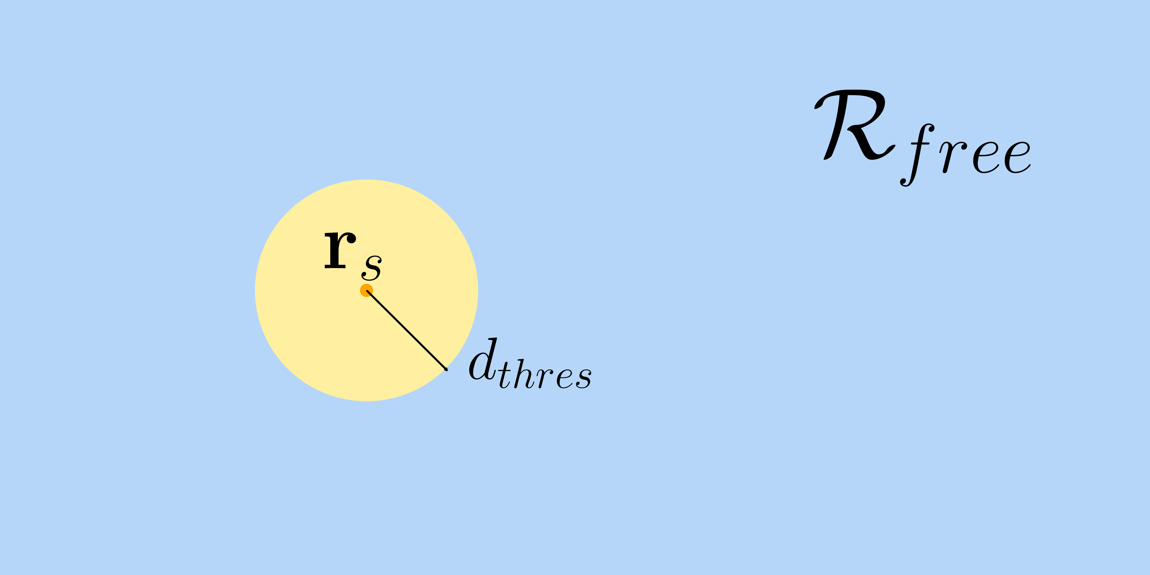
A collision means entering a prescribed separation threshold around the satellite. Each predicted time step must keep debris outside that region with probability at least 1 − ε. MPC minimizes a weighted quadratic control-effort sum, used as a fuel proxy, subject to the nonlinear dynamics and these chance constraints. The initial debris state is Gaussian, but its future distribution need not be. The constraints are marginal per-step bounds: the formulation does not allocate a single ε across the entire horizon or establish continuous-time safety between evaluated states. The quadratic objective is also distinct from the total Δv reported in the plots.
Equation 4
| (4) |
Equations 5–6e
| (5) |
| (6a) | ||||
| (6b) | ||||
| (6c) | ||||
| (6d) | ||||
| (6e) | ||||
5 Preliminaries
The derivation separates three ideas: uncertainty over distributions, conversion of a collision event into a scalar loss, and conservative replacement of its quantile by a tail-risk measure.
5.1 Distributionally Robust Chance Constraints
The ambiguity set contains candidate debris distributions. Enforcing safety for the worst member implies safety under the true distribution only if the true distribution belongs to that set. This condition is explicit in Equation 7. Replacing exact moments by estimates does not automatically preserve containment; no confidence region for moment-estimation error is constructed here.
Equation 7
| (7) |
5.2 Chance Constraints and their CVaR Approximations
A safety loss is nonpositive on the selected safe region. The chance constraint is expressed as a bound on its upper-tail Value-at-Risk. CVaR is defined through the threshold-plus-expected-excess optimization in Equation 10; because it bounds VaR, requiring CVaR ≤ 0 is sufficient for the chance constraint. Taking the worst CVaR over the ambiguity set extends that implication to distributional robustness [17]. These implications are conservative, not equalities between collision probability and CVaR.
The source’s following unnumbered “conditional expectation” display is malformed: it writes an expectation of an inequality rather than a conditional tail-loss expression. Equation 10 is the operative definition; a naive conditional-tail expectation also needs care when distributions have atoms. The original display is retained for fidelity rather than silently repaired.
Equations 8–12
| (8) |
| (9) |
| (10) |
| (11) |
| (12) |
6 Risk-Sensitive Collision Avoidance using Distributionally Robust Chance Constraints
A convex quadratic loss produces a closed-form worst-case CVaR condition. The remaining trajectory optimization is nonlinear, and the authors solve it with a constrained cross-entropy search.
6.1 Reformulation of Chance Constraint by Distributionally Robust CVaR Constraints
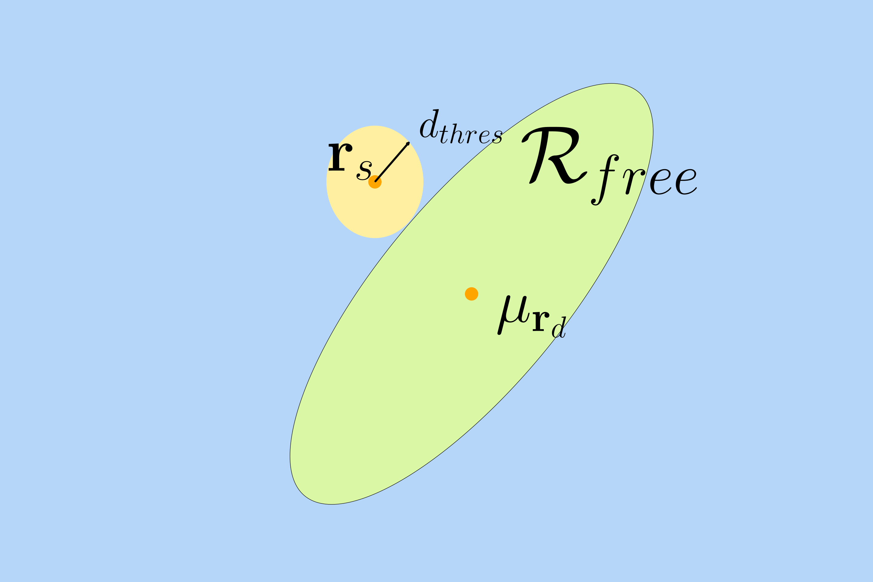
At each time step, the ambiguity set fixes the debris position mean μ and covariance Σ. The geometric safe set is an ellipsoid centered on μ and contained outside the satellite’s collision ball, with loss (r − μ)ᵀE(r − μ) − 1 and positive-definite E. Theorem 1 gives worst-case CVaR as −1 + tr(ΣE)/ε, so the sufficient condition is tr(ΣE) ≤ ε. The proof is delegated to Corollary 1.3 of the cited robust-control work [17]. Smaller ε, greater covariance, or a smaller safe ellipsoid makes the condition stricter.
The ellipsoid is a conservative subset of allowed debris positions, not the collision obstacle itself. Its placement relative to each candidate satellite position is essential to the collision guarantee. The paper illustrates this geometry but does not give a complete numerical construction of E from the satellite position and clearance threshold, which limits implementation reproducibility. Convexity of the loss in debris position does not make the nonlinear MPC problem globally convex.
Equations 13
| (13) |
Equations 14–16e
| (14) |
| (15) |
| (16a) | ||||
| (16b) | ||||
| (16c) | ||||
| (16d) | ||||
| (16e) | ||||
6.2 Constrained Cross-Entropy Method
CEM samples control sequences, rolls out satellite dynamics, and rejects sequences violating the trace constraint. The lowest-effort feasible sequences form an elite set that updates the sampling distribution. If no feasible sequence exists, elites minimize a discounted sum of the per-step CVaR expressions to guide the search toward safer candidates [18]. This fallback is a search heuristic: negative values at some steps can offset violations elsewhere, and a fixed iteration budget does not guarantee eventual feasibility. The paper does not specify a certified backup action if the final search remains infeasible.
Algorithm 1 is retained in full. Its rollout line prints the initial debris state where the surrounding text calls for the satellite state; this apparent notation error is left visible. Candidate counts, elite fraction, iteration budget, runtime, and convergence evidence are not reported, so onboard computational performance is not established.
Input Current satellite state , Initial debris state distribution
Output Control input for satellite
Equation 17
| (17) |
7 Experiment Settings
Evaluation uses one close-approach scenario derived from public orbital records. All three uncertainty propagators feed the same robust MPC formulation.
7.1 Satellite-Debris Collision Scenario
7.1.1 Identification of Spacecraft and System Constraints
The authors select a close approach from SOCRATES Plus on CelesTrak [19], retrieve the objects’ NORAD identifiers and Two-Line Elements, and reproduce their trajectories in MATLAB. The predicted conjunction supplies a realistic starting scenario, while the subsequent dynamics, noise, masses, and actuation limits are simulation choices.
7.1.2 Collision Scenario Setup
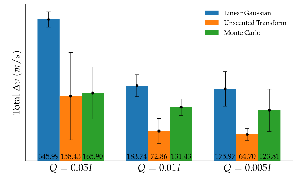
The pair is Starlink 52579 and the unpropelled THEA 43796, treated as debris. The nominal closest range is 41 m, and the avoidance threshold is 100 m. Assumed masses are 300 kg and 50 kg. The text specifies white debris process noise with Q = 0.05I, acceleration bounds of ±0.05 km/s² per axis, a 0.01 s dynamics step, replanning every second, a 10 s horizon, and ε = 0.05. The acceleration limit equals 50 m/s² per axis; the authors explicitly choose unusually high thrust and a short horizon to expose parameter effects. These settings are not an operationally validated fuel-efficient satellite maneuver design.
7.2 Uncertainty Propagation
The implementations differ only in how future debris moments are approximated. Distributional robustness is conditional on those supplied moments for all three methods.
7.2.1 Linear Propagation of Gaussian Uncertainty
The nominal nonlinear dynamics propagate the mean. A linearized state-transition matrix propagates covariance as APAᵀ plus discrete process-noise covariance; the upper-left position block becomes Σ. This is inexpensive, but neglected nonlinear effects can distort both covariance magnitude and direction.
Equations
7.2.2 Unscented Transform
For a six-dimensional state, the source constructs thirteen sigma points around the initial mean, propagates them through nonlinear dynamics, and estimates their mean and covariance. This can capture effects absent from linear covariance propagation. The printed sigma-point formula applies chol to an already square-rooted covariance expression, despite defining chol itself as a Cholesky decomposition. That ambiguous notation is preserved; it should be resolved against an implementation before reproducing the method.
Equations 19a–19b
| (19a) | ||||
| (19b) | ||||
7.2.3 Monte Carlo Uncertainty Propagation
Monte Carlo propagation samples 50 initial states and simulates nonlinear trajectories, then uses sample moments rather than directly counting rare collisions. This avoids requiring those 50 trajectories to resolve the desired tail probability, but 50 samples do not make the estimated moments exact. The paper provides no finite-sample correction or confidence bounds for their errors. Its qualitative preference for Monte Carlo is supported by this simulation comparison, not a universal guarantee that a small sample estimate dominates every alternative.
8 Simulation Results
Results report closest separation and maneuver Δv, with ten trials per parameter setting and mean/standard-deviation bars. They show risk-cost trends rather than measured collision frequencies or a statistical test of chance-constraint satisfaction.
8.1 Result of Uncertainty Propagation and Collision Avoidance Maneuver
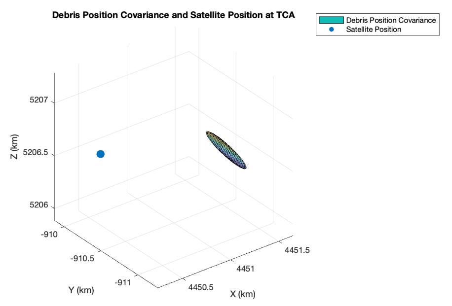
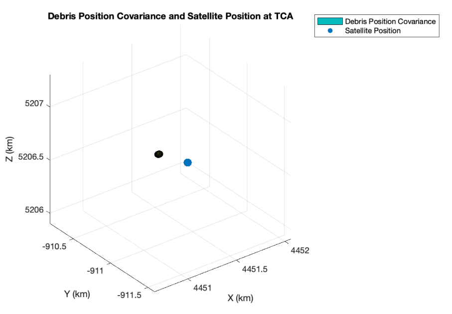
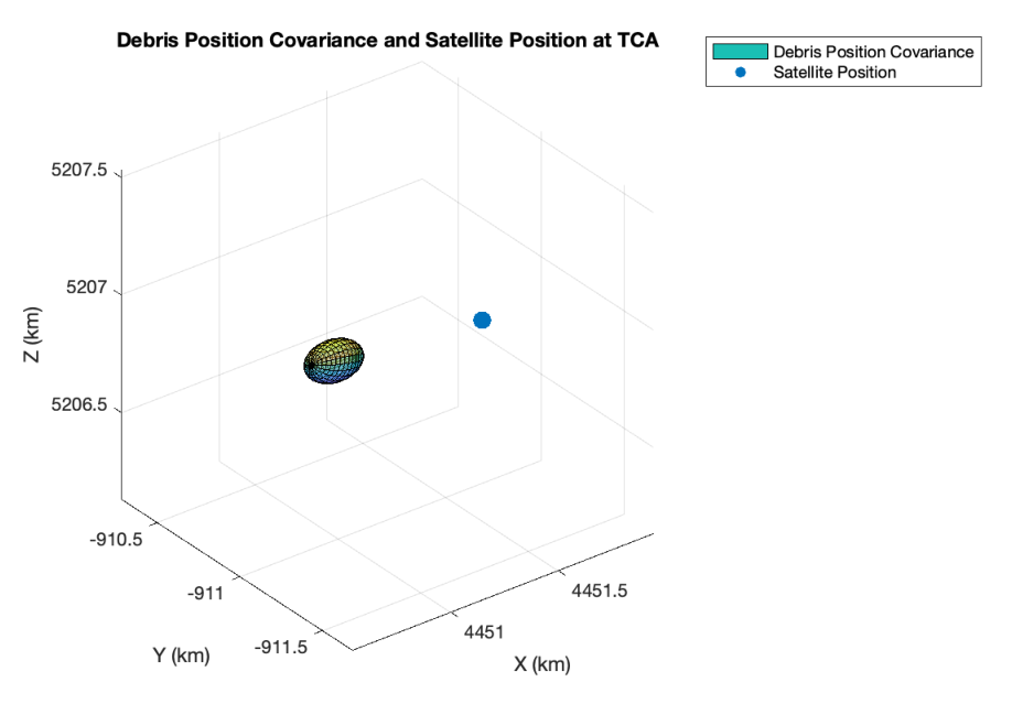
At closest approach, the linear propagator gives a differently oriented covariance and a different maneuver. Unscented propagation resembles the Monte Carlo shape but estimates less spread. Figure 3 preserves all three covariance/position panels. The qualitative comparison demonstrates sensitivity to propagation quality; robustification over distribution shape cannot repair incorrect moment estimates.
8.2 Effect of Chance Constraint Probability
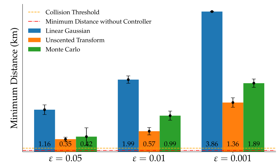
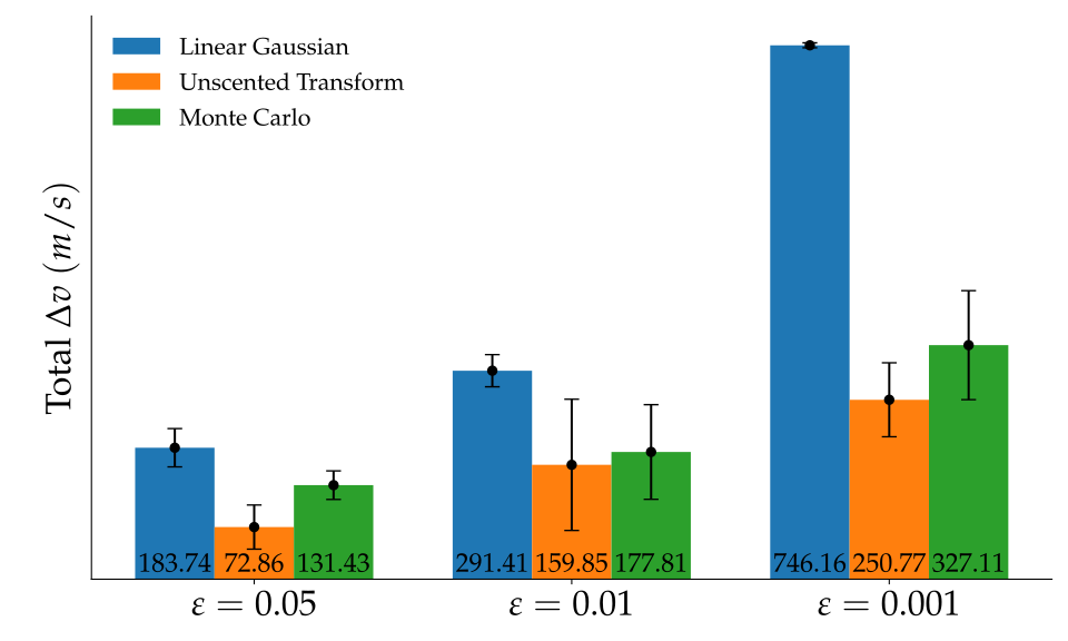
Reducing ε from 0.05 to 0.001 increases separation and Δv. Figure 4’s Monte Carlo means rise from 0.42 to 1.89 km and from 131.43 to 327.11 m/s; linear propagation rises from 1.16 to 3.86 km and from 183.74 to 746.16 m/s. The unscented method is less costly in these runs. All plotted mean separations exceed the 0.1 km threshold, but mean clearance and ten repetitions cannot certify low collision probabilities or establish an optimum across avoidance methods.
8.3 Effect of Uncertainty in Debris Dynamics
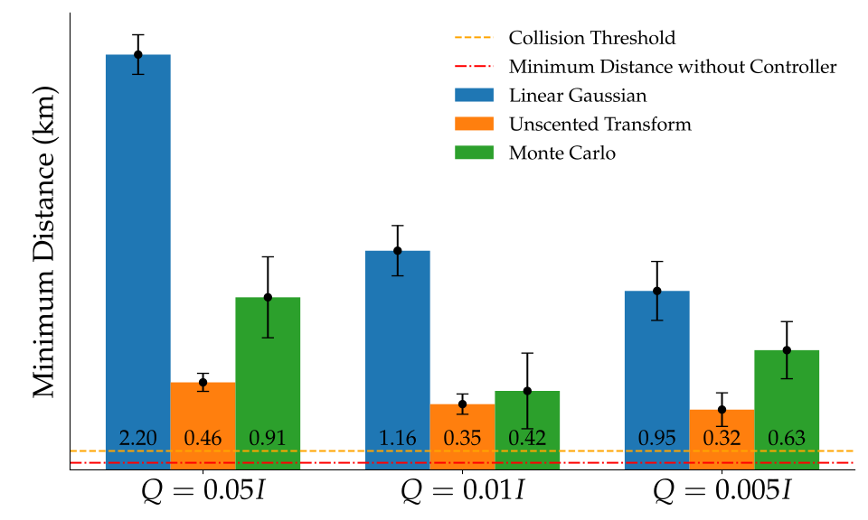
Figure 5 varies Q over 0.05I, 0.01I, and 0.005I. Smaller assumed process noise generally reduces required separation and Δv; Monte Carlo means change from 0.91 to 0.63 km and from 165.90 to 123.81 m/s. The Monte Carlo mean clearance is not monotonic: it is 0.42 km at the middle noise level. This is a sensitivity analysis to the assumed uncertainty model. The baseline values in Figure 4 at ε = 0.05 match Figure 5 at Q = 0.01I, whereas the setup text names Q = 0.05I; the paper does not explain that discrepancy.
9 Conclusion and Future Work
The central contribution is a tractable moment-based risk constraint that can accept several uncertainty propagators. Its guarantees require correct moments, safe ellipsoid geometry, and a feasible computed solution. Evidence is limited to one simulated pair, a deterministic controlled satellite, ten trials per setting, and deliberately aggressive actuation. There is no empirical rare-event validation, runtime benchmark, full-horizon risk guarantee, or comparison against other avoidance controllers. More efficient optimization and multiple-object avoidance are proposed future work.
Acknowledgments
The authors acknowledge National Science Foundation support under ECCS-2438314, CNS-2423130, and CCF-2423131.