SCDS learns trajectory-generating policies from state demonstrations using contractive recurrent equilibrium networks and invertible output layers. The architecture supports ordinary gradient optimization and an adjustable contraction rate. Simulated handwriting, navigation, and manipulation tests show lower errors from perturbed starting states. The paper also presents loss bounds for a bounded initial-state region; these concern the modeled trajectories and rely on stated mathematical and controller assumptions.
1 Introduction
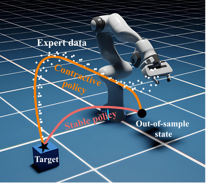
Asymptotic convergence can permit large transient deviations from demonstrations. SCDS instead promotes contraction between trajectories. It combines a recurrent equilibrium network (REN), a learned latent space, and coupling layers, training on complete state rollouts rather than measured velocities. The intended benefit is faster recovery toward demonstrated behavior after a change of initial state. [11], [19], [38].
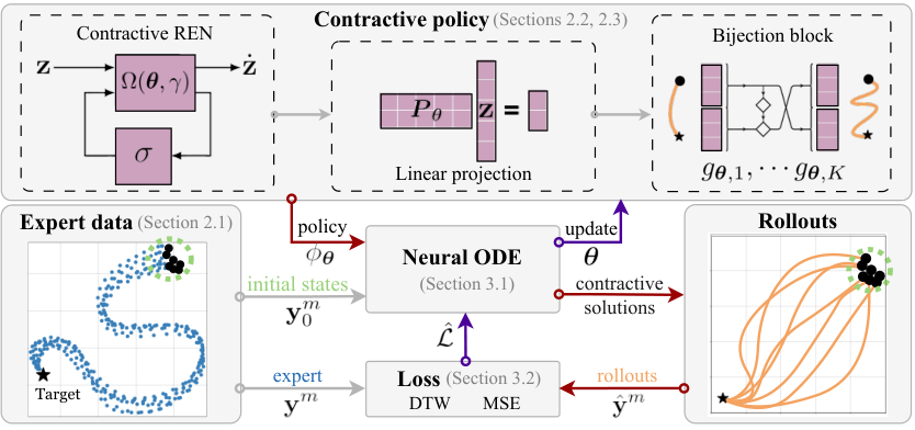
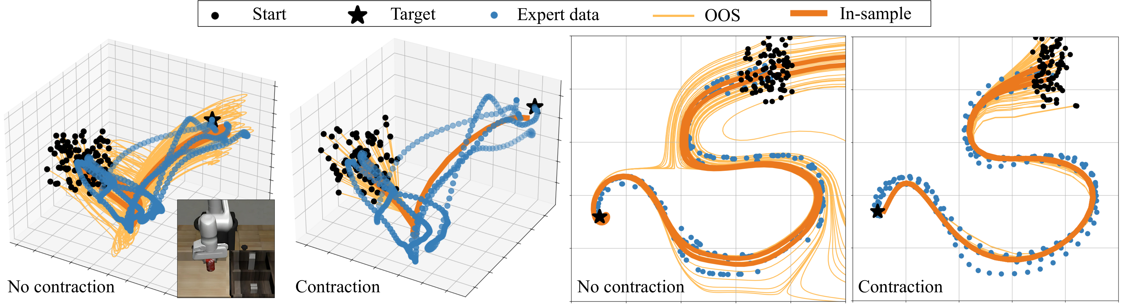
Figure 1: Policy rollouts generated by contractive and stable policies. While both policies eventually reach the target, the contractive policy closely mimics the expert in the transient phase.Figure 2: Overview of the SCDS training scheme. The policy structure (top box) consists of a REN, a linear projection, and a bijection block, ensuring contractivity for any choice of parameters, . In the forward pass (→), initial states are passed through a differentiable ODE solver to generate state rollouts. The loss function penalizes the discrepancy between the generated and expert trajectories, updating the policy via backpropagation (←).
2 Contractive Policy Formulation
The policy consists of latent dynamics, an initialization map, and an output transformation.
2.1 Problem Setup
Training data and the desired recovery behavior define the learning problem.
Dataset.
Demonstrations contain sampled states with potentially different lengths and initial conditions. The formal setup assumes a common target and does not require state derivatives as training labels.
Equation 1
(1)
Objective.
The objective combines faithful reproduction with recovery from unseen initial states or perturbations. Stability of the trajectory generator is the proposed mechanism.
2.2 Background: Contractive latent dynamics
A continuous REN parameterization guarantees exponential convergence of latent trajectories for its allowed activation functions and constructed matrices. The rate can be prescribed or learned. Its implicit nonlinear state is required to be uniquely defined. [41].
Equations 2–3
(2)
(3)
2.3 Expressive Contractive Policies
A learned linear projection changes latent dimension, and invertible coupling layers add nonlinear output flexibility. Initialization inverts these layers and applies a pseudoinverse, potentially only approximating the requested state. The authors state that the output preserves contraction and its rate. A separate low-level controller must track the generated states on the robot.
Equations 4–7
(4)
(5)
(6)
(7)
3 Learning Contractive Policies through Imitation
Training differentiates through policy rollouts and measures their discrepancy from expert state trajectories.
A differentiable ODE solver produces rollouts over a selected horizon; multiple initial conditions can be integrated in parallel. Longer horizons increase computation and memory demands.
3.2 Trajectory space loss
MSE compares aligned, equal-length trajectories, while soft-DTW accommodates temporal alignment and unequal lengths. A proposed inverse-distance weighting emphasizes demonstrations with nearby starting states. Experiments use rollouts initialized at demonstration starts and average their corresponding imitation losses. [38].
Equation 8
(8)
Figure 3: Uniform weighting averages the deviation from both demonstrations, hence, .
In contrast, Eq. 9 results in . For , the weights in Eq. 9 assign higher importance to the closer ’s demonstration, which is intuitive.Equations 9–10
(9)
(10)
3.3 Optimization problem
Gradient descent minimizes the trajectory loss without adding separate contraction constraints, because the REN parameterization supplies its latent stability structure. Algorithm 1 retains the training sequence and optional contraction-rate optimization.
The authors state worst-case and expected MSE bounds for equal-length rollouts whose initial states lie in a bounded multifocal-ellipse region around demonstration starts. The bound separates training error from an initial-state uncertainty term controlled by region size and contraction constants. It does not directly certify soft-DTW loss, task completion, collision avoidance, or low-level tracking.
Equations 12
(12)
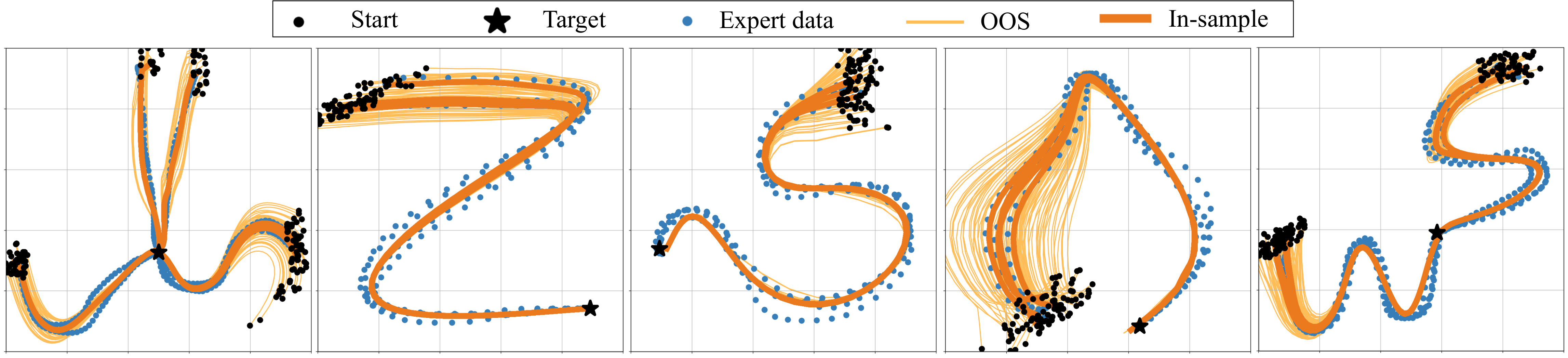
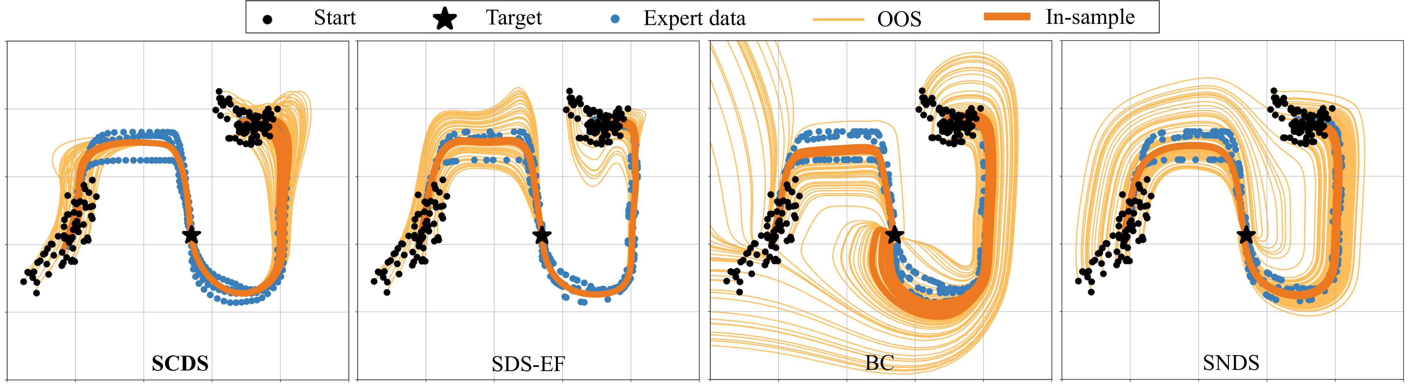
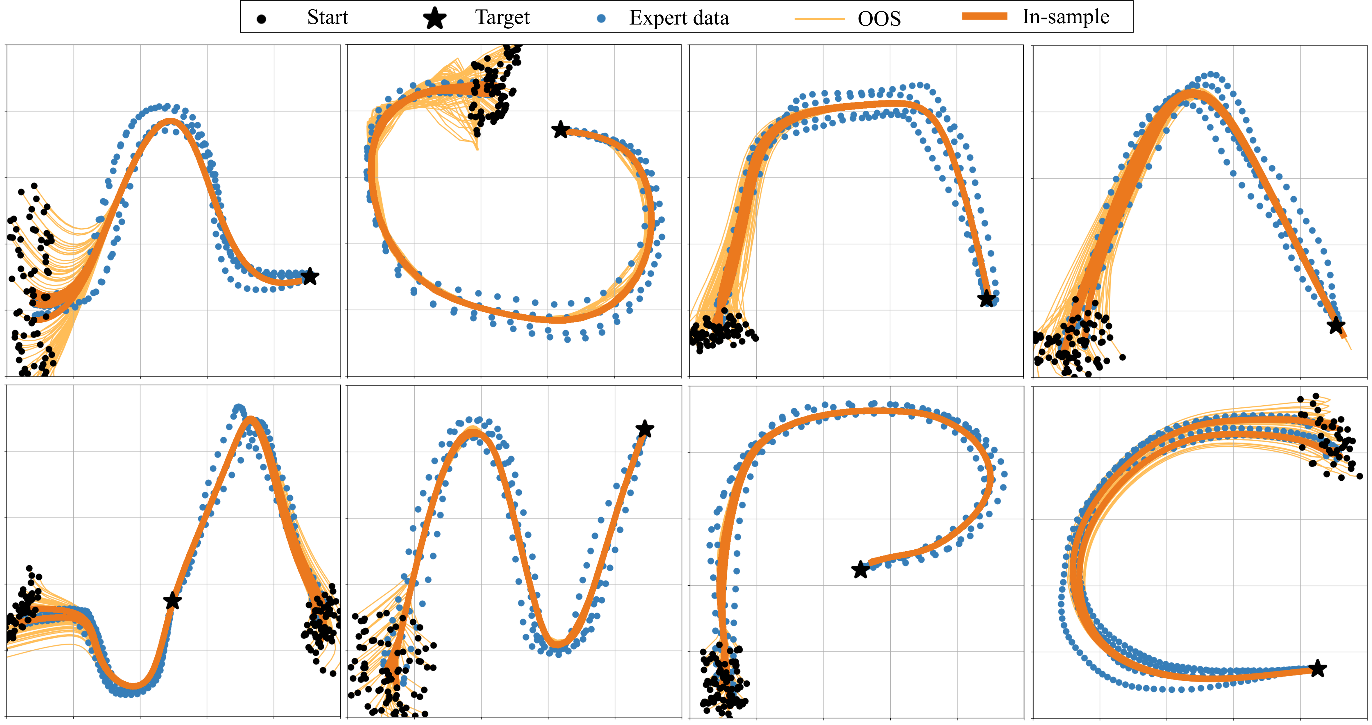
Figure 4: In-sample and OOS policy rollouts for selected 2D tasks in the LASA dataset. The training process promotes higher contraction rates ( App. E.2), resulting in effective OOS recovery.Figure 5: Comparing SCDS to the selected baselines on in-sample and OOS rollouts in the 2D task space. BC results in diverging trajectories due to the lack of stability guarantees. While SNDS and SDS-EF ensure global stability and reach the target, they display large deviations from expert data. In contrast, SCDS efficiently recovers from OOS states through its contracting transient behavior.Equation
5 Experiments
Experiments use LASA handwriting and Robomimic demonstrations, followed by simulated deployment in Isaac Lab.
5.1 Setup and baselines
Baselines are SNDS, SDS-EF, and ordinary behavior cloning. Out-of-sample starts are sampled near demonstrated starts, with radius 10% of their norm. MSE and soft-DTW measure trajectory error. The paper compares state-only SCDS with baselines trained using state derivatives.
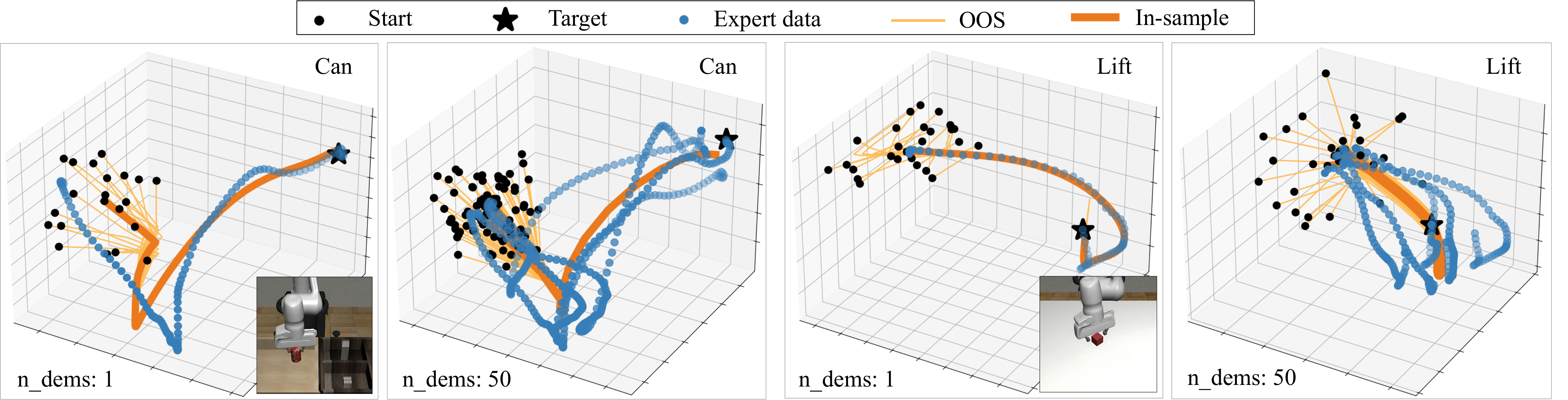
Figure 6: In-sample and OOS policy rollouts for the 6D Can and Lift tasks in the Robomimic dataset, using both and demonstrations. SCDS generates contractive trajectories even in higher-dimensional spaces, where expert trajectories exhibit non-converging patterns.
5.2 Results and discussion
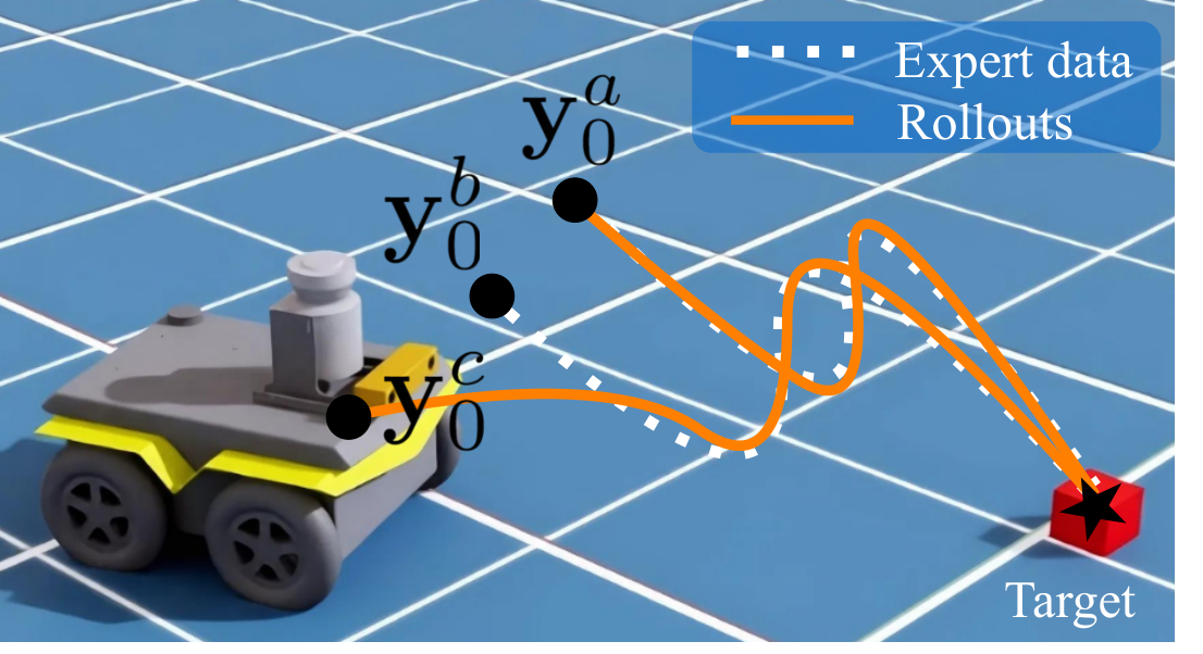
SCDS has the lowest reported out-of-sample errors across the four benchmark representations. Robomimic-14D MSE is 2.68 ± 0.65 versus the best baseline’s 6.88 ± 2.16; in-sample advantages are smaller and not universal. Some Robomimic demonstrations have different endpoints, departing from the formal common-target assumption. Reported numerical bounds use an empirically estimated contraction constant. Franka and Jackal deployment tests are simulated, with 50 starting states each.
6 Conclusion, Limitations, and Future work
Contraction-focused trajectory learning improves recovery in the reported tests, at the cost of longer training and sensitivity to horizon choices. The method assumes a suitable low-level controller. Broader robot classes, longer tasks, and stochastic policies are proposed extensions rather than demonstrated results.
Table 1: Evaluating in-sample and out-of-sample rollouts error on the LASA and the Robomimic datasets.
The lowest (best) values for each metric and dataset are highlighted. The expressive power of SCDS enables it to achieve near state-of-the-art performance on in-sample data. More notably, it consistently outperforms other baselines in OOS recovery, and conforms with the theoretical upper bound for MSE loss, , as derived in Sec. 4.
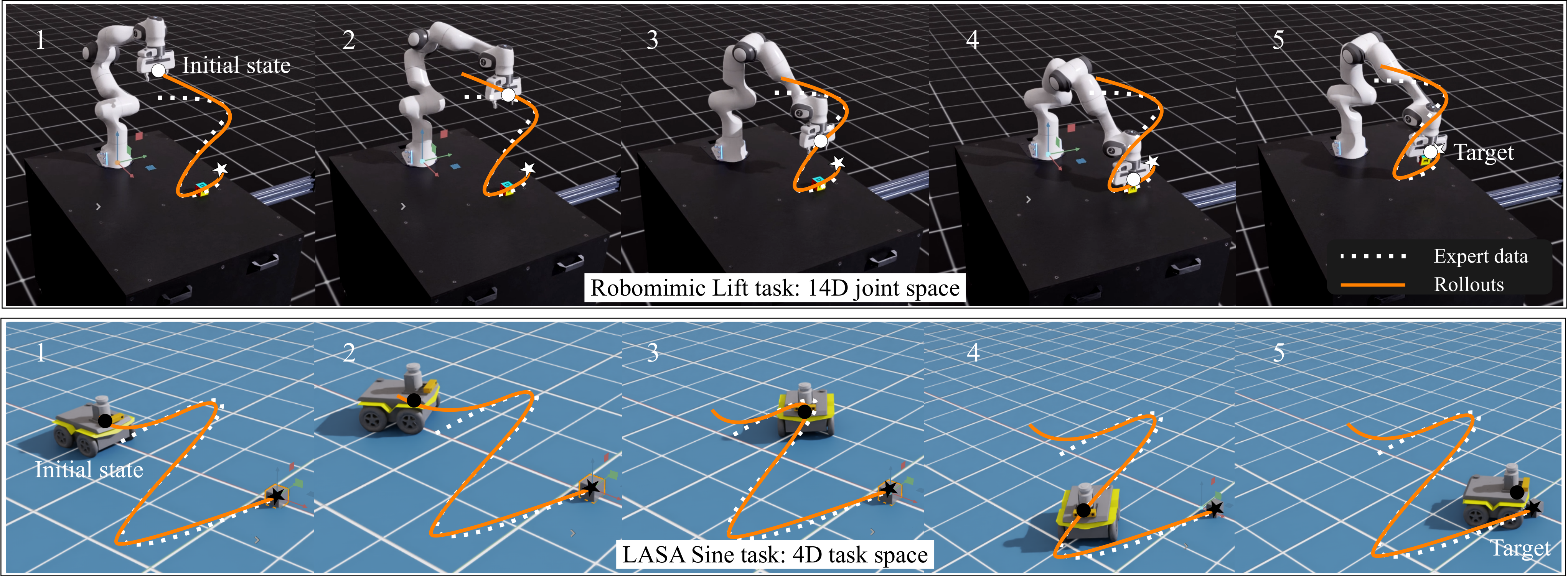
Figure 7: Simulation rollouts with Franka arm and Jackal mobile robots in Isaac Lab. Both robots start from a random OOS initial state and swiftly converge to expert data.
Acknowledgments
Support came from NCCR Automation and the NECON project through the Swiss National Science Foundation.
Appendix
The appendices retain proofs, design choices, ablations, implementation details, and datasets.
Appendix A Mathematical proofs
The authors provide derivations for output contraction and the proposed loss bounds.
A.1 Proposition 2.1
The proof combines a singular-value bound for the linear projection with a coordinate-change argument for bijective layers. Its displayed constant divides by a minimum singular value, so a nonzero lower bound is required for that argument; rank-deficient projections need separate care.
Equations 13
(13)
A.2 Theorem 4.1
The proposed loss proof combines initial-state weighting, an exponential trajectory bound, and a harmonic–arithmetic mean inequality. Equation 16 invokes a triangle inequality for MSE; squared Euclidean loss does not satisfy the ordinary triangle inequality in general. The displayed bound is retained as the paper’s stated result rather than an independently established certificate.
Equations 14–20
(14)
(15)
(16)
(17)
(18)
(19)
(20)
A.3 Corollary 4.1.1
The expected-loss result follows from the stated pointwise bound by replacing a weighted training error with its maximum and taking expectation over the allowed initial-state region.
Equations 21
(21)
Appendix B Extended related work
The related-work comparison separates constrained contraction methods from architectures with built-in structure.
Table 2: Comparing contractive DS methods for imitation learning. Except for NCDS and SCDS, the rest attempt to solve a computationally challenging constrained optimization problem.
B.1 Stable dynamical policies with restricted representations
Earlier Lyapunov-based approaches restrict either the motion field or certificate to make optimization tractable. Learning more flexible certificates can improve expressiveness but complicates joint optimization.
B.2 Stable neural dynamical policies
Neural stable policies use coordinate transformations or projection-based enforcement. The authors contrast their contraction objective with these asymptotic-stability approaches and their representation or smoothness limitations.
B.3 Imitation policies with no stability guarantees
Adversarial imitation, noise injection, and dataset aggregation address imitation and distribution shift through different mechanisms. They do not provide the particular contraction certificate targeted here.
RENs supply a flexible family of implicit dynamical models with structured stability properties. SCDS uses the continuous-time formulation, with a discrete variant also implemented.
Appendix C Design considerations
Several choices trade imitation accuracy against recovery speed and computational cost.
C.1 Contraction rate
A larger contraction rate accelerates convergence between rollouts but restricts expressiveness. Nonlinear output layers help recover modeling flexibility.
C.2 Horizon
Longer integration horizons resolve intricate or longer motions at greater training cost. Solver choice and numerical tolerance also affect this trade-off.
Soft-DTW replaces the discrete minimum over alignments with a differentiable soft minimum. Its smoothing parameter controls approximation to ordinary DTW.
Equation 23
(23)
C.4 Implicit depth and invertible layers
Increasing the REN implicit-state dimension adds capacity but can be expensive. The authors favor additional invertible output layers for a more efficient expressiveness increase.
The appendix summarizes prior continuous-REN results used by the architecture.
D.1 Detailed structure
The general REN includes state, input, output, and implicit nonlinear variables. SCDS removes external inputs and biases and replaces the original output equation with its learned projection and coupling layers.
Equations 24–25
(24)
(25)
D.2 Universal contraction
Positive-definite matrix conditions provide the cited sufficient condition for contraction of the latent REN.
Equations
D.3 Free parameterization and constructability
A free parameterization constructs the needed positive-definite matrices from Gram matrices and diagonal margins, allowing unconstrained optimization of the underlying parameters.
Latent trajectories converge faster at higher rates. When the LASA start-region radius increases from 10% to 25% of the demonstrated initial-state norm, SCDS retains the lowest reported errors: MSE 0.57 in 2D and 1.44 in 4D.
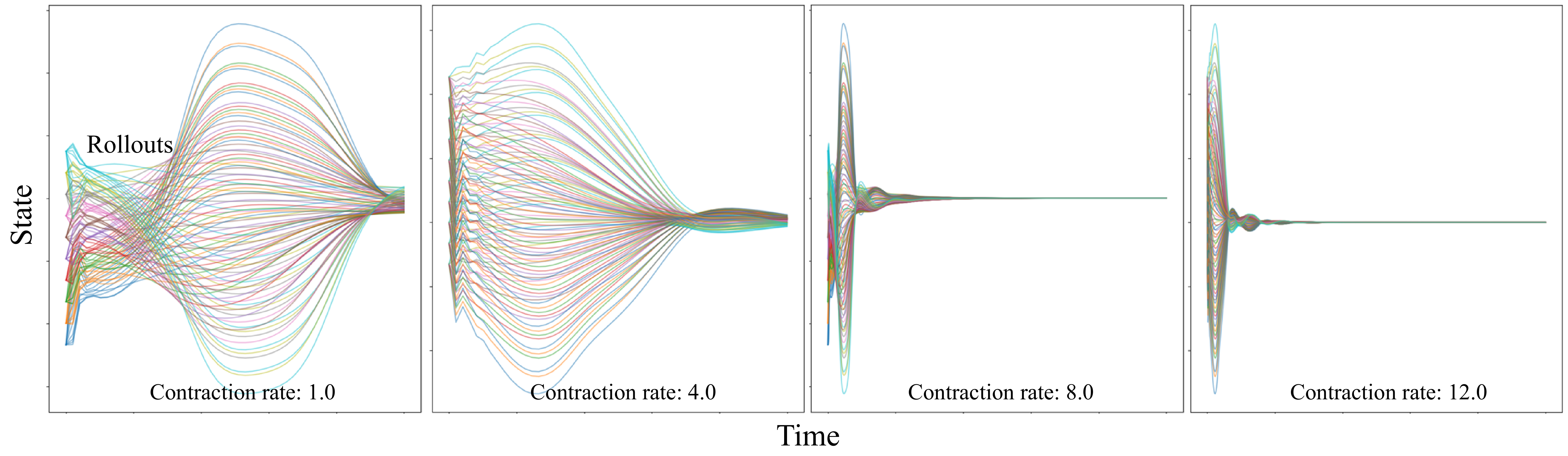
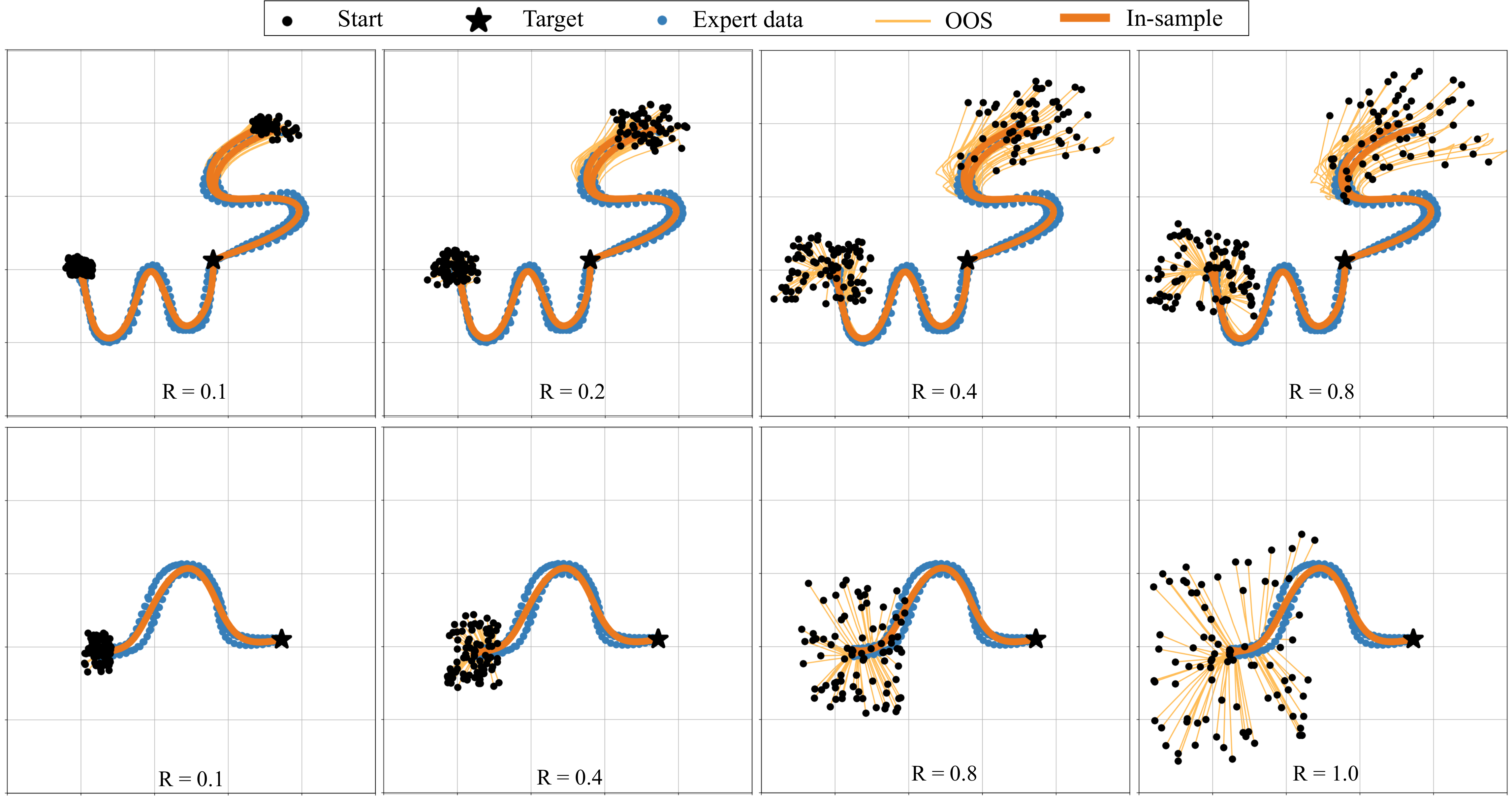
Figure 8: Contractive behavior of the latent state. The figure illustrates the rollouts over time for varying dimensions of the latent state, under different contraction rates. Higher contraction rates accelerate convergence in both the latent state space and the robot’s state space. The dimension of the latent state here is set to 10.Figure 9: SCDS is tested over additional motions in the LASA dataset. In all cases, the induced trajectories accurately imitate the expert, even for out-of-sample initial states.Figure 10: Out-of-sample recovery for initial states sampled from regions with different volumes according to the definition of in Assumption 4.1. Notably, SCDS recovers even from more distant initial states.
Table 3: Evaluating out-of-sample rollouts error on the LASA dataset. Compared to Table 1, the OOS initial states are sampled from a wider distribution with a radius of for the LASA dataset.
The lowest (best) values for each metric and dataset are highlighted. These results confirm that the recovery behavior observed in Fig. 10 persists across all the other tasks in the LASA dataset.
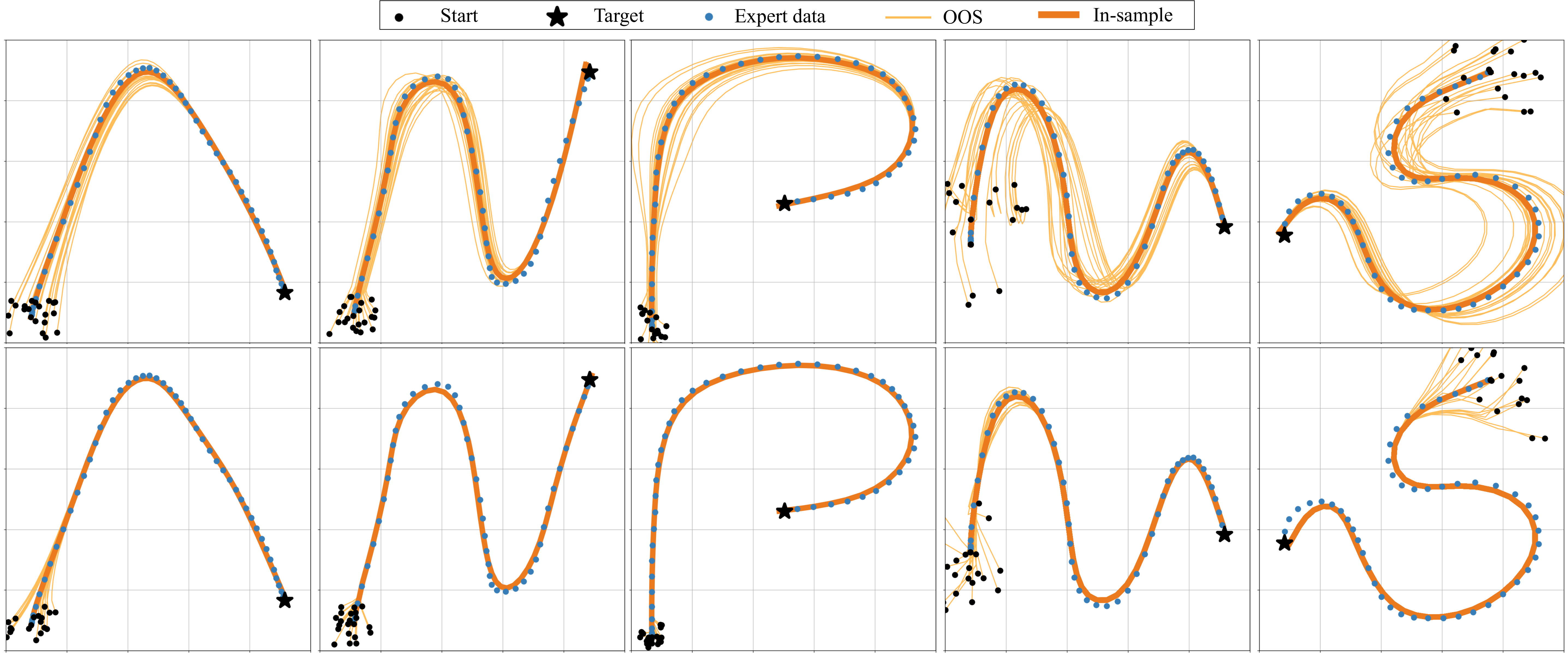
An augmented objective is used to encourage larger learned contraction rates. The plotted examples recover more quickly than policies trained at a low fixed rate.
Equation 26
(26)
Figure 11: Policies trained to have low (first row) and high (second row) contraction rates. SCDS can promote higher contraction rates during training to achieve more robustness to out-of-sample initial states and perturbations.
E.3 Latent state dimension
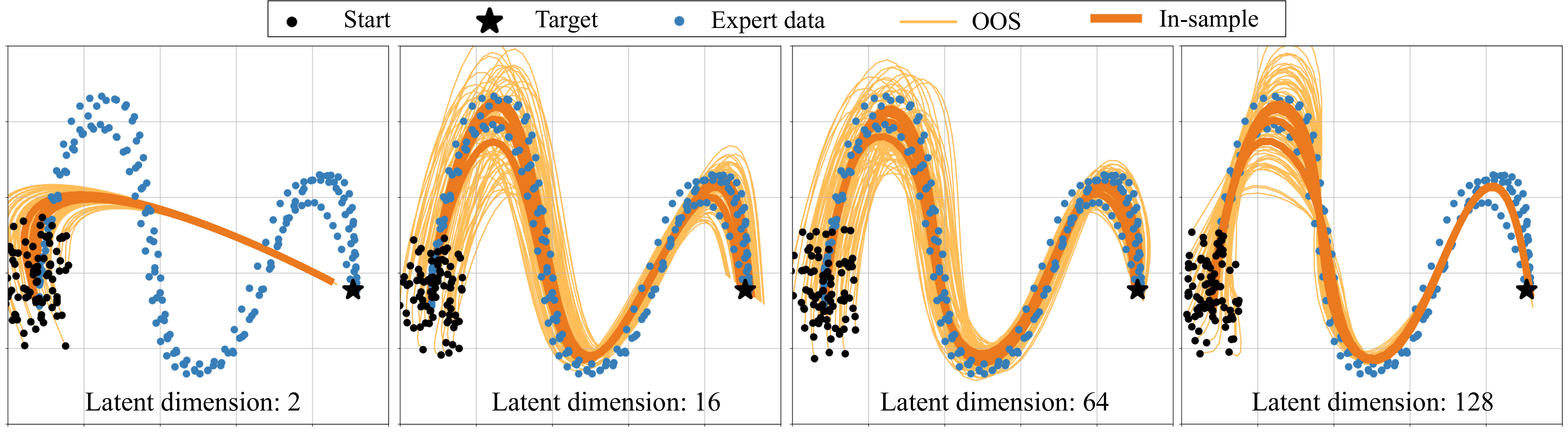
Larger latent states improve imitation of the selected complex handwriting motion. A small latent model can remain stable while fitting demonstrations poorly.
Figure 12: Training results for a sample motion in the LASA dataset are plotted for various latent space dimensions. Training in higher dimensional latent space is more effective, especially when facing complex expert behavior that involves multiple demonstrations. Note that the time horizon is fixed here for all the rollouts.
E.4 Ablation study: bijective layers
Removing bijective output layers worsens reconstruction. Increasing REN complexity without those layers can recover comparable accuracy, but trains more slowly in the reported comparison.
Table 4: Ablation study on invertible layers to improve the policy’s expressive power. SCDS is the standard policy formulation presented in Eq. 7. SCDS-NB uses the same REN structure but does not have bijection layers. SCDS-NB∗ makes SCDS-NB more complex by increasing the complexity of the implicit layer in the REN architecture. Still SCDS-NB∗ uses no invertible layers. The best results are displayed for 50 trials on in-sample initial states.
E.5 Ablation study: replacing REN with a non-contractive model
Replacing the contractive REN with an unconstrained RNN produces diverging out-of-sample trajectories in the illustrated tasks, supporting the role of the latent contraction structure.
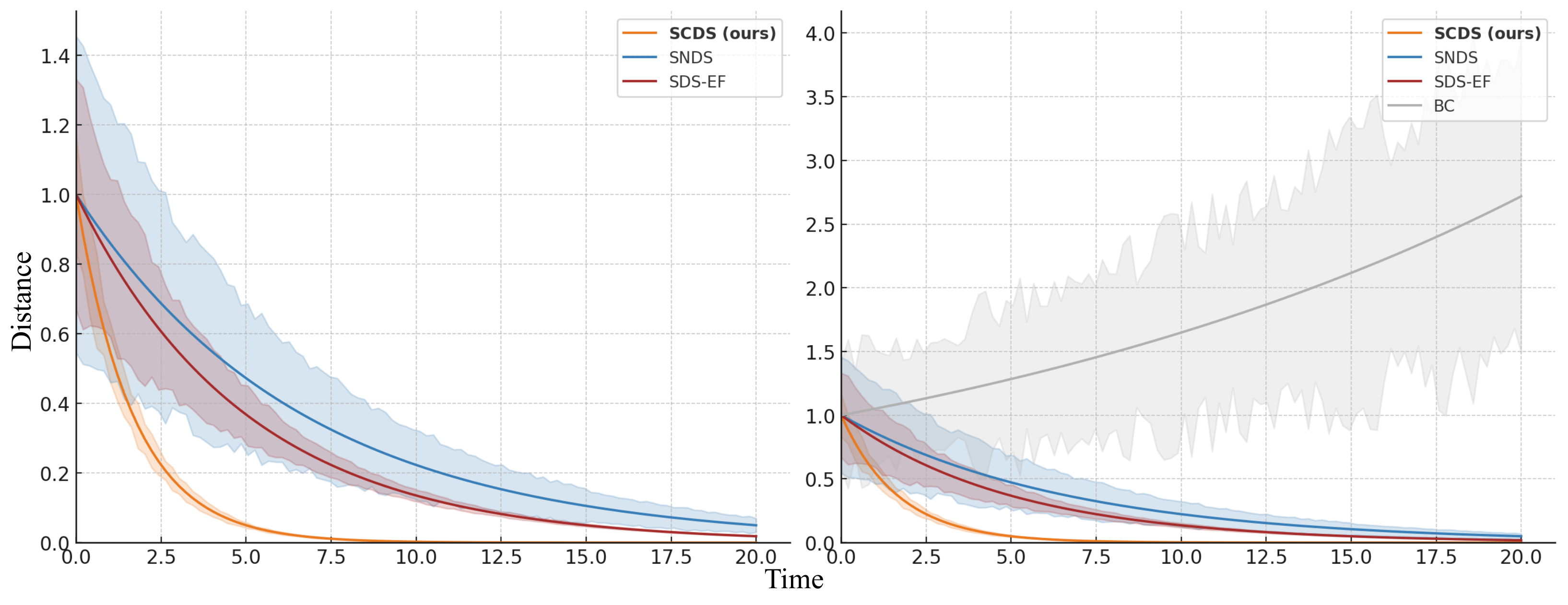
Figure 13: The effect of replacing the contractive REN with a non-contractive model, specifically a recurrent neural network, is investigated across two candidate tasks. Some of the generated trajectories diverge in the no contraction case, which lacks guarantees on out-of-sample recovery.Figure 14: Distance between induced trajectories for the policies using a contractive REN (left) and a non-contractive RNN (right), with a uniformly distributed set of initial states around the true initial conditions from the LASA dataset. Since the policy in the right figure is not contractive or stable, the trajectories begin to diverge, causing the distance between neighboring trajectories to increase.
E.6 Computation time
At equal epoch and data counts, continuous SCDS trains substantially more slowly than the baselines: about 1,795 seconds for LASA-2D and 2,711 seconds for Robomimic-14D. Discrete SCDS is faster but uses more memory. The authors note that equal epochs do not imply equal convergence progress.
Table 5: Evaluating the training time on the LASA and the Robomimic datasets in seconds. SCDS using either discrete or continuous REN architecture appears to be less computationally efficient in lower dimensions, but will shorten the gap in efficiency in larger datasets. Note that even though the same number of epochs are used here, the continuous SCDS method typically requires less than half of the number of epochs to achieve the same performance. Although SCDS has longer training times, it offers the stronger contractivity guarantee compared to the stability guarantees of the stable baselines or the lack of any guarantees in the case of BC.
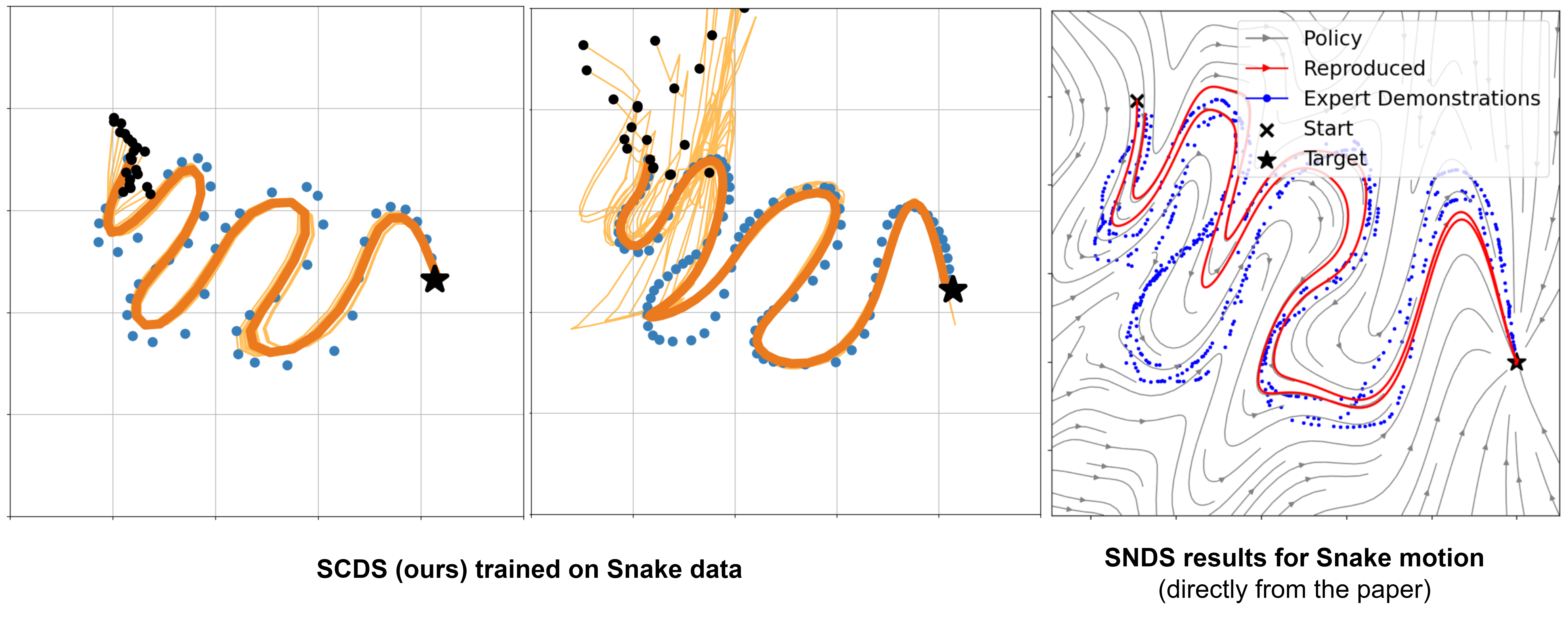
On a longer Snake motion, reported DTW errors are 0.074 at a low rate and 0.097 at a higher rate, compared with approximately 0.158 reported for SNDS. This illustrates a recovery-speed versus imitation-accuracy trade-off.
Figure 15: SCDS results for the Snake dataset demonstrate its ability to handle a more complex motion compared to the tasks in the LASA dataset. SCDS is applied starting from closer (left plot) and further (middle plot) initial conditions and is compared against SNDS (right plot). The complexity of the Snake task arises from the Snake dataset’s longer time horizon and the need for rapid adaptation in DS learning.
Appendix F Implementation details
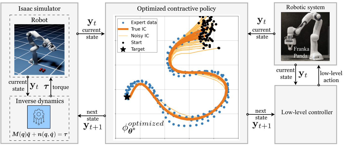
The implementation uses PyTorch and a trajectory-generation interface to robot controllers. The deployment diagram includes real-world possibilities, while the reported robot experiments are simulations.
Figure 16: Simulation and real-world deployment pipelines. The trained policy can be deployed to both real and simulated robots with minimal effort. Global stability and highly contractive behavior of induced trajectories ensure safety and precision during these zero-shot transfers.
The main components are the REN, invertible coupling layers, and differentiable trajectory loss.
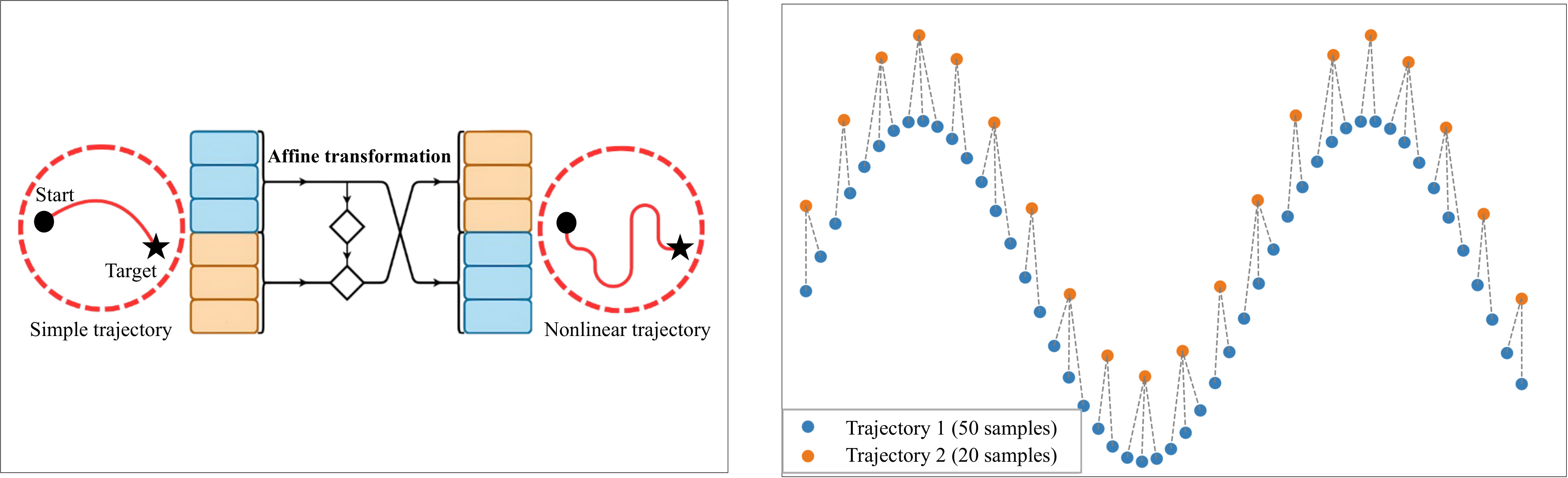
Figure 17: Left: Invertible coupling layer structure implemented as a part of RealNVP. The affine transformation provides increased nonlinearity while maintaining bijection, and as a result, contraction properties. Right: DTW still effectively compares trajectories with different lengths. This is particularly useful when learning long-horizon trajectories, or dealing with higher sampling rates.
Continuous RENs support ODE integration at arbitrary times and adjoint-based gradients. Discrete RENs avoid an ODE solver and can be faster, with a gradient graph that grows with horizon length.
(2) Invertible coupling layers
RealNVP coupling layers keep one input partition fixed while using it to parameterize an invertible affine transformation of the other.
(3) Soft and differentiable dynamic time warping
Soft-DTW aligns trajectories with different speeds, lengths, or sample rates, providing a differentiable alternative to directly aligned MSE.
F.2 Baselines
The authors reuse and tune existing baseline implementations. They do not compare directly with NCDS, citing the absence of an official implementation at the time.
The BC baseline is a feedforward or residual state-to-action model rather than recurrent BC. Tables 6 and 7 retain code sources, architectures, and SCDS parameter ranges, including 32–64 latent dimensions and 20–50 rollout steps.
Table 6: Baseline implementation, architecture, and hyperparameters
Table 7: Hyperparameters of SCDS and their optimal values or ranges are shown for every key model parameter.
Param
Description
Optimal value(s)
Lower bound on the contraction rate of the policy
, learnable
Number of coupling layer to increase the output nonlinearity
Dimension of the latent state space
Forward simulation horizon for the generated trajectory
Number of invertible layers in the output map (also used for hidden blocks)
Complexity-accuracy trade-off parameter for soft-DTW ( in some references)
F.3 Computational resources
Training uses an RTX 4090 GPU and a machine with 64 GBRAM. Isaac Lab simulations run remotely and exploit parallel environments.
F.4 Simulation in Isaac Lab
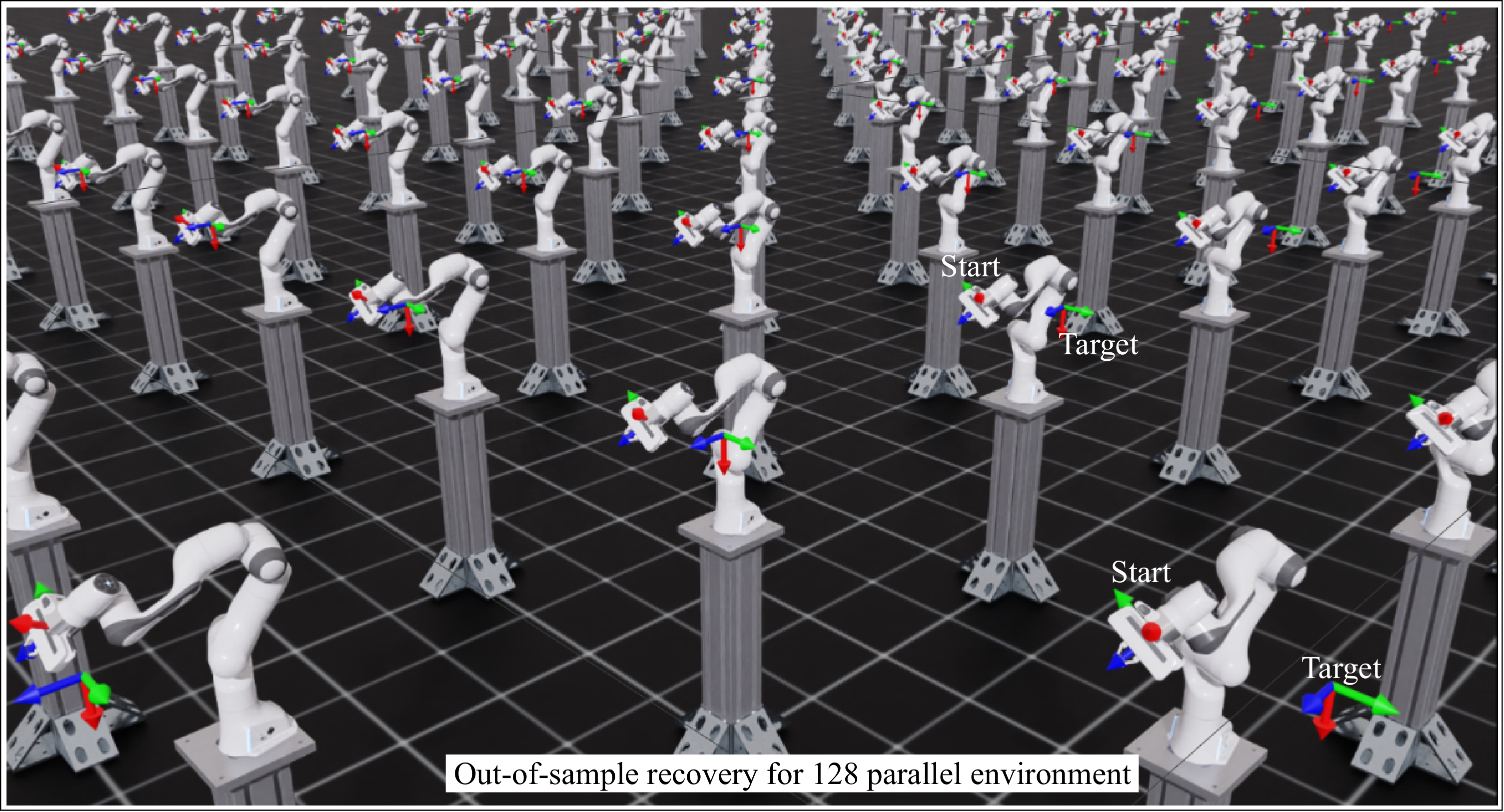
Isaac Lab evaluates randomized robot initial conditions in parallel. Generated states are converted to the required joint or task-space commands; the reported benchmark evaluation uses 128 sampled starts.
Figure 18: Efficient parallel testing of out-of-sample behavior in the Isaac Lab robotics simulator. Each robot is given a random initial condition drawn from a uniform distribution around true initial states. The parallel testing of 128 sampled initial conditions yields the results in Tab. 1.
F.5 Low-level controller
The formulation assumes a low-level controller capable of tracking the generated state sequence. Joint-position, inverse-dynamics, or inverse-kinematics controllers supply the connection to motor commands; the trajectory-generator analysis alone does not establish closed-loop tracking accuracy.
Appendix G Datasets
The datasets cover low-dimensional handwriting and higher-dimensional robot configurations.
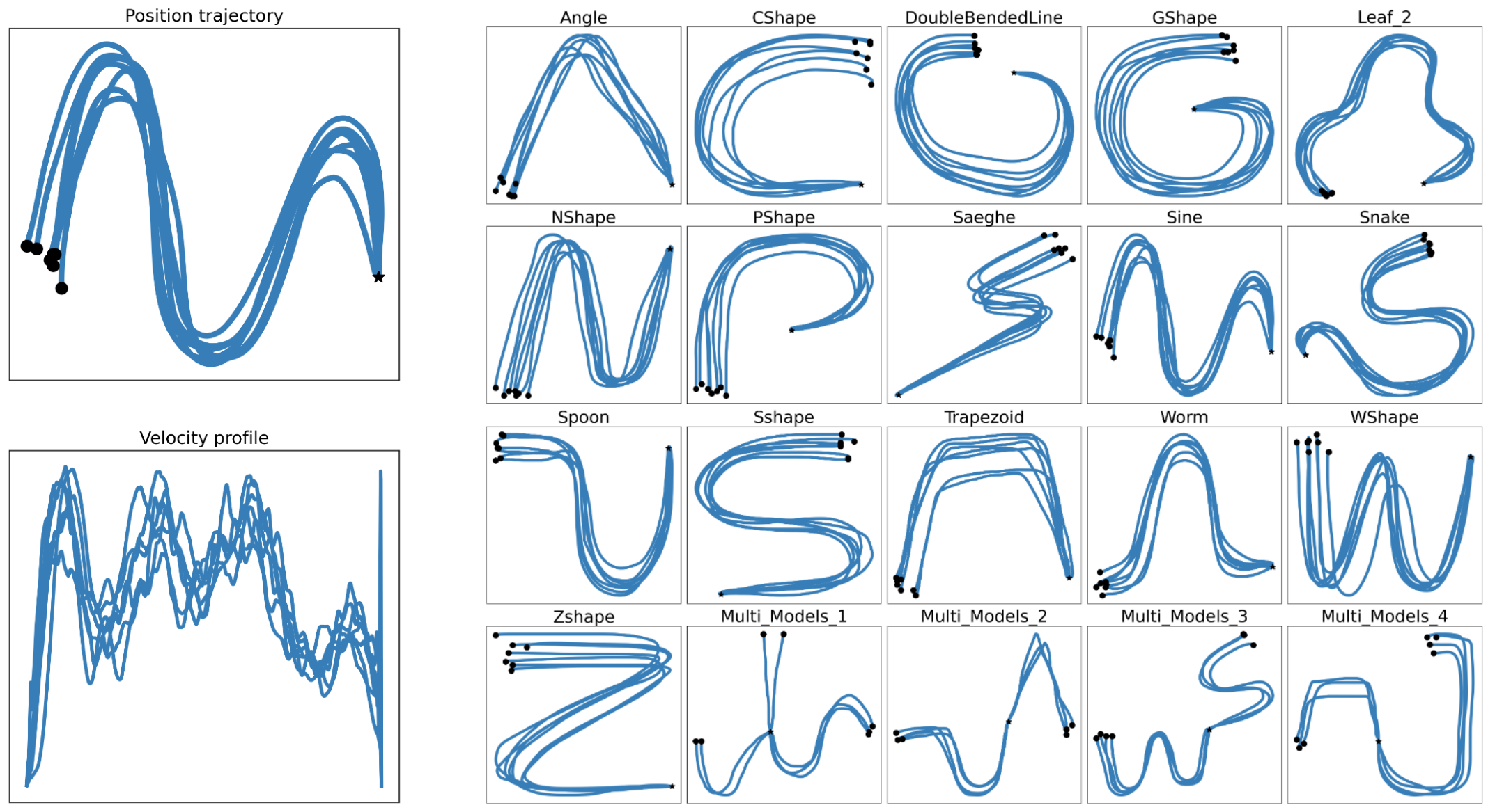
LASA provides seven demonstrations per handwriting motion with 1,000 samples each and common endpoints. Soft-DTW allows much shorter generated rollouts during fitting.
Figure 19: Expert demonstrations in the LASA dataset.
G.2 Robomimic dataset
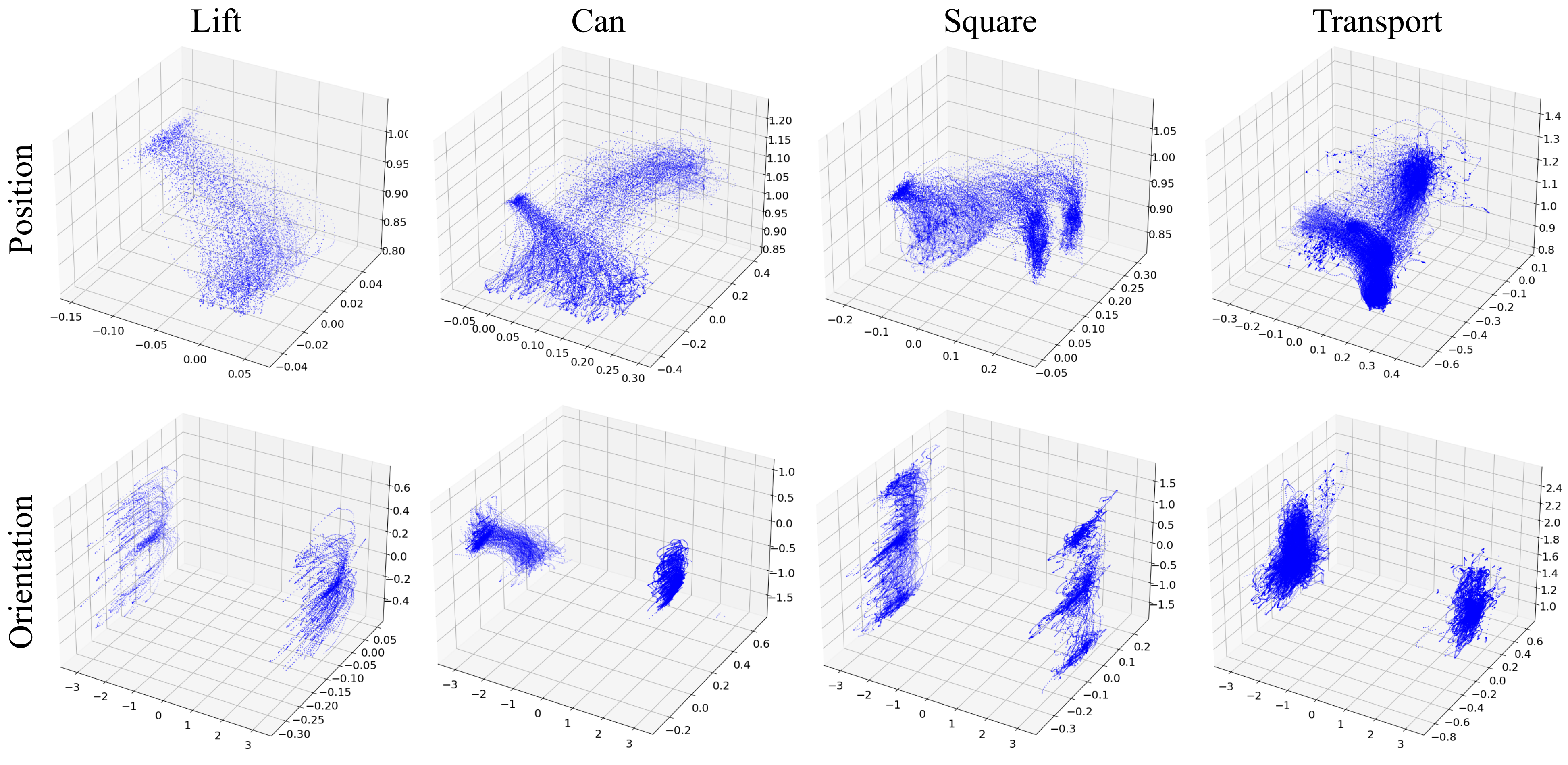
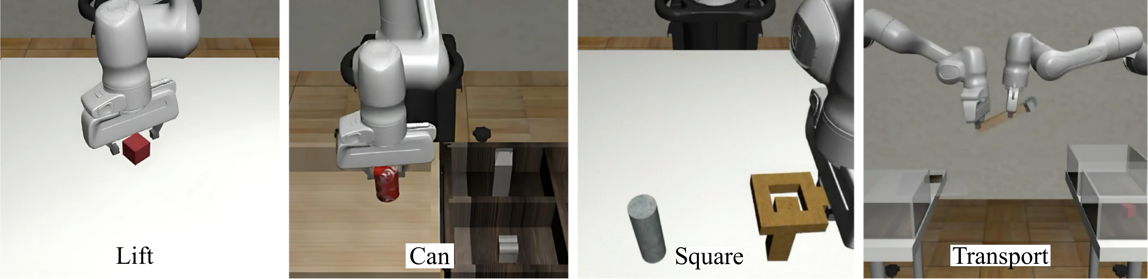
Robomimic experiments use Lift, Can, Square, and Transport demonstrations. End-effector position and orientation give six-dimensional states; seven joint positions and velocities give fourteen. The authors generally train on 80–90% of the 200–300 demonstrations per task and reserve the remainder for evaluation.
Figure 20: Position and orientation data for different tasks in the Robomimic dataset. Figure 21: Data collection setup for Lift, Can, Square, and transport tasks (Mandlekar et al., 2021). We employ this collected data, which is available in the Robomimic repository.
50 references
Abbeel & Ng (2004)
Pieter Abbeel and Andrew Y Ng.
Apprenticeship learning via inverse reinforcement learning.
In International Conference on Machine Learning, pp. 1, 2004.
Abyaneh & Lin (2023)
Amin Abyaneh and Hsiu-Chin Lin.
Learning Lyapunov-stable polynomial dynamical systems through imitation.
In 7th Annual Conference on Robot Learning, 2023.
Abyaneh et al. (2024)
Amin Abyaneh, Mariana Sosa Guzmán, and Hsiu-Chin Lin.
Globally stable neural imitation policies.
In IEEE International Conference on Robotics and Automation (ICRA), pp. 15061–15067, 2024.
Bahl et al. (2020)
Shikhar Bahl, Mustafa Mukadam, Abhinav Gupta, and Deepak Pathak.
Neural dynamic policies for end-to-end sensorimotor learning.
Advances in Neural Information Processing Systems, 33:5058–5069, 2020.
Blocher et al. (2017)
Caroline Blocher, Matteo Saveriano, and Dongheui Lee.
Learning stable dynamical systems using contraction theory.
In 14th International Conference on Ubiquitous Robots and Ambient Intelligence (URAI), pp. 124–129, 2017.
Boroujeni et al. (2021)
Mahrokh Ghoddousi Boroujeni, Elham Daneshman, Ludovic Righetti, and Majid Khadiv.
A unified framework for walking and running of bipedal robots.
In 2021 20th International Conference on Advanced Robotics (ICAR), pp. 396–403. IEEE, 2021.
Boroujeni et al. (2024)
Mahrokh Ghoddousi Boroujeni, Clara Lucía Galimberti, Andreas Krause, and Giancarlo Ferrari-Trecate.
A PAC-Bayesian framework for optimal control with stability guarantees.
arXiv preprint arXiv:2403.17790, 2024.
Chen et al. (2018)
Ricky TQ Chen, Yulia Rubanova, Jesse Bettencourt, and David K Duvenaud.
Neural ordinary differential equations.
Advances in Neural Information Processing Systems, 31, 2018.
Chi et al. (2023)
Cheng Chi, Zhenjia Xu, Siyuan Feng, Eric Cousineau, Yilun Du, Benjamin Burchfiel, Russ Tedrake, and Shuran Song.
Diffusion policy: Visuomotor policy learning via action diffusion.
The International Journal of Robotics Research, pp. 02783649241273668, 2023.
Cuturi & Blondel (2017)
Marco Cuturi and Mathieu Blondel.
Soft-DTW: a differentiable loss function for time-series.
In International Conference on Machine Learning, pp. 894–903. PMLR, 2017.
Dawson et al. (2023)
Charles Dawson, Sicun Gao, and Chuchu Fan.
Safe control with learned certificates: A survey of neural lyapunov, barrier, and contraction methods for robotics and control.
IEEE Transactions on Robotics, 39(3):1749–1767, 2023.
Dinh et al. (2017)
Laurent Dinh, Jascha Sohl-Dickstein, and Samy Bengio.
Density estimation using real NVP.
In International Conference on Learning Representations, 2017.
Figueroa & Billard (2018)
Nadia Figueroa and Aude Billard.
A physically-consistent bayesian non-parametric mixture model for dynamical system learning.
In 2nd Annual Conference on Robot Learning, pp. 927–946, 2018.
Fu et al. (2018)
Justin Fu, Katie Luo, and Sergey Levine.
Learning robust rewards with adversarial inverse reinforcement learning.
In International Conference on Learning Representations, 2018.
Ho & Ermon (2016)
Jonathan Ho and Stefano Ermon.
Generative adversarial imitation learning.
Advances in Neural Information Processing Systems, 29:4572–4580, 2016.
Keogh & Ratanamahatana (2005)
Eamonn Keogh and Chotirat Ann Ratanamahatana.
Exact indexing of dynamic time warping.
Knowledge and Information Systems, 7:358–386, 2005.
Khansari-Zadeh & Billard (2011)
S Mohammad Khansari-Zadeh and Aude Billard.
Learning stable nonlinear dynamical systems with Gaussian mixture models.
IEEE Transactions on Robotics, 27(5):943–957, 2011.
Khansari-Zadeh & Billard (2014)
S Mohammad Khansari-Zadeh and Aude Billard.
Learning control Lyapunov function to ensure stability of dynamical system-based robot reaching motions.
Robotics and Autonomous Systems, 62(6):752–765, 2014.
Laskey et al. (2017)
Michael Laskey, Jonathan Lee, Roy Fox, Anca Dragan, and Ken Goldberg.
DART: Noise injection for robust imitation learning.
In 1st Conference on Robot Learning, 2017.
Manchester & Slotine (2015)
Ian R. Manchester and Jean-Jacques E. Slotine.
Control contraction metrics: Convex and intrinsic criteria for nonlinear feedback design.
IEEE Transactions on Automatic Control, 62:3046–3053, 2015.
Mandlekar et al. (2020)
Ajay Mandlekar, Danfei Xu, Roberto Martín-Martín, Silvio Savarese, and Li Fei-Fei.
GTI: Learning to Generalize across Long-Horizon Tasks from Human Demonstrations.
In Proceedings of Robotics: Science and Systems, Corvalis, Oregon, USA, July 2020.
Mandlekar et al. (2021)
Ajay Mandlekar, Danfei Xu, Josiah Wong, Soroush Nasiriany, Chen Wang, Rohun Kulkarni, Li Fei-Fei, Silvio Savarese, Yuke Zhu, and Roberto Martín-Martín.
What matters in learning from offline human demonstrations for robot manipulation.
In 5th Annual Conference on Robot Learning, 2021.
Martin & Furieri (2024)
Andrea Martin and Luca Furieri.
Learning to optimize with convergence guarantees using nonlinear system theory.
IEEE Control Systems Letters, 2024.
Martinelli et al. (2023)
Daniele Martinelli, Clara Lucía Galimberti, Ian R. Manchester, Luca Furieri, and Giancarlo Ferrari-Trecate.
Unconstrained parametrization of dissipative and contracting neural ordinary differential equations.
In 2023 62nd IEEE Conference on Decision and Control (CDC), pp. 3043–3048, 2023.
Menda et al. (2019)
Kunal Menda, Katherine Driggs-Campbell, and Mykel J. Kochenderfer.
EnsembleDAgger: A bayesian approach to safe imitation learning.
In 2019 IEEE/RSJ International Conference on Intelligent Robots and Systems (IROS), pp. 5041–5048, 2019.
Mohammadi et al. (2024)
Hadi Beik Mohammadi, Søren Hauberg, Georgios Arvanitidis, Nadia Figueroa, Gerhard Neumann, and Leonel Rozo.
Neural contractive dynamical systems.
In The Twelfth International Conference on Learning Representations, 2024.
Neumann & Steil (2015)
Klaus Neumann and Jochen J Steil.
Learning robot motions with stable dynamical systems under diffeomorphic transformations.
Robotics and Autonomous Systems, 70:1–15, 2015.
Papamakarios et al. (2021)
George Papamakarios, Eric Nalisnick, Danilo Jimenez Rezende, Shakir Mohamed, and Balaji Lakshminarayanan.
Normalizing flows for probabilistic modeling and inference.
Journal of Machine Learning Research, 22(57):1–64, 2021.
Paszke et al. (2019)
Adam Paszke, Sam Gross, Francisco Massa, Adam Lerer, James Bradbury, Gregory Chanan, Trevor Killeen, Zeming Lin, Natalia Gimelshein, Luca Antiga, Alban Desmaison, Andreas Kopf, Edward Yang, Zachary DeVito, Martin Raison, Alykhan Tejani, Sasank Chilamkurthy, Benoit Steiner, Lu Fang, Junjie Bai, and Soumith Chintala.
PyTorch: An imperative style, high-performance deep learning library.
In H. Wallach, H. Larochelle, A. Beygelzimer, F. d'Alché-Buc, E. Fox, and R. Garnett (eds.), Advances in Neural Information Processing Systems 32, pp. 8024–8035. Curran Associates, Inc., 2019.
Peng et al. (2019)
Xue Bin Peng, Angjoo Kanazawa, Sam Toyer, Pieter Abbeel, and Sergey Levine.
Variational discriminator bottleneck: Improving imitation learning, inverse RL, and GANs by constraining information flow.
In International Conference on Learning Representations, 2019.
Penrose (1956)
R. Penrose.
On best approximate solutions of linear matrix equations.
Mathematical Proceedings of the Cambridge Philosophical Society, 52(1):17–19, 1956.
doi: 10.1017/S0305004100030929.
Pomerleau (1988)
Dean A Pomerleau.
ALVINN: An autonomous land vehicle in a neural network.
In Advances in Neural Information Processing Systems, volume 1, pp. 305–313, 1988.
Rana et al. (2020)
Muhammad Asif Rana, Anqi Li, Dieter Fox, Byron Boots, Fabio Ramos, and Nathan Ratliff.
Euclideanizing flows: Diffeomorphic reduction for learning stable dynamical systems.
In Learning for Dynamics and Control, pp. 630–639. PMLR, 2020.
Ravichandar et al. (2017)
Harish Ravichandar, Iman Salehi, and Ashwin Dani.
Learning partially contracting dynamical systems from demonstrations.
In 1st Annual Conference on Robot Learning, 2017.
Ravichandar et al. (2020)
Harish Ravichandar, Athanasios S Polydoros, Sonia Chernova, and Aude Billard.
Recent advances in robot learning from demonstration.
Annual review of control, robotics, and autonomous systems, 3(1):297–330, 2020.
Revay et al. (2023)
Max Revay, Ruigang Wang, and Ian R Manchester.
Recurrent equilibrium networks: Flexible dynamic models with guaranteed stability and robustness.
IEEE Transactions on Automatic Control, 2023.
Ross & Bagnell (2010)
Stéphane Ross and Drew Bagnell.
Efficient reductions for imitation learning.
In Proceedings of the thirteenth international conference on artificial intelligence and statistics, pp. 661–668. JMLR Workshop and Conference Proceedings, 2010.
Sochopoulos et al. (2024)
Andreas Sochopoulos, Michael Gienger, and Sethu Vijayakumar.
Learning deep dynamical systems using stable neural ODEs.
In Proceedings of the 2024 IEEE/RSJ International Conference on Intelligent Robots and Systems, 2024.
Tabak & Turner (2013)
Esteban G Tabak and Cristina V Turner.
A family of nonparametric density estimation algorithms.
Communications on Pure and Applied Mathematics, 66(2):145–164, 2013.
Torabi et al. (2018)
Faraz Torabi, Garrett Warnell, and Peter Stone.
Behavioral cloning from observation.
In Proceedings of the 27th International Joint Conference on Artificial Intelligence, pp. 4950–4957, 2018.
Tsukamoto et al. (2021)
Hiroyasu Tsukamoto, Soon-Jo Chung, and Jean-Jaques E Slotine.
Contraction theory for nonlinear stability analysis and learning-based control: A tutorial overview.
Annual Reviews in Control, 52:135–169, 2021.
Vincze (1982)
P. Erdös I. Vincze.
On the approximation of convex, closed plane curves by multifocal ellipses.
Journal of Applied Probability, 19(A):89–96, 1982.
Zhang et al. (2022)
Jiechao Zhang, Hadi Beik Mohammadi, and Leonel Rozo.
Learning Riemannian stable dynamical systems via diffeomorphisms.
In 6th Annual Conference on Robot Learning, 2022.
Ziebart et al. (2008)
Brian D Ziebart, Andrew L Maas, J Andrew Bagnell, Anind K Dey, et al.
Maximum entropy inverse reinforcement learning.
In Association for the Advancement of Artificial Intelligence, volume 8, pp. 1433–1438, 2008.