At a glance
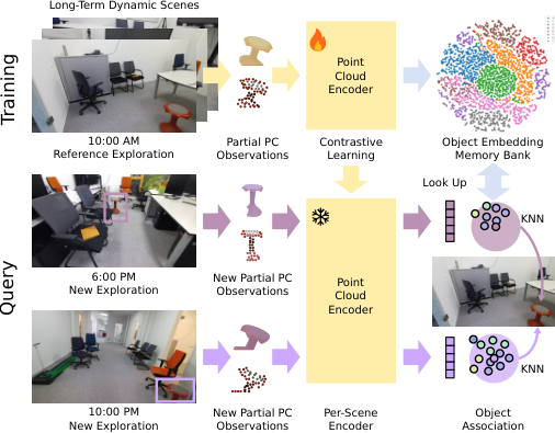
BYE trains an object point-cloud encoder separately for each scene, using partial views collected during one reference exploration. Contrastive learning groups views of the same object, and a memory bank supports matching objects after they move. Adding these instance-specific scores to CLIP features reaches 95.6% association success in simulation and 100% in two small real-world settings. The main gain is complementary identity information: the per-scene encoder alone does not beat CLIP overall in simulation.
I Introduction
The target is change between visits: an object can move while the robot is absent, yet remain stationary during each exploration. A useful map must reconnect new observations to old individual objects, not merely recognize their categories. BYE replaces synthetic shape/category training with one scene’s own observations. Inspired by per-scene representation learning in LangSplat [10], it builds a compact encoder and retains embeddings of partial views. “Class-agnostic” means no predefined category vocabulary; consistent object-instance labels are still required during training.
II Related Work
Open-vocabulary mapping attaches visual-language features to places, voxels, objects, or implicit fields, but often assumes a static scene. Dynamic SLAM commonly filters or tracks currently moving objects; longer-term change methods register revisited scenes or use pretrained shape models. BYE instead learns a scene-specific identity representation. PointNet [36] and DGCNN [37] supply alternative point-cloud backbones, while SimCLR [43] motivates contrastive training. The study tests association, not open-vocabulary language queries, general dynamic reconstruction, or navigation.
III Problem Definition
Each exploration provides RGB images, depth, instance masks, and camera poses. These reconstruct one point cloud per object. Given reference and revisited object sets, the goal is a bijection between their identities. The formulation assumes equal-sized sets after excluding newly added or removed objects, and objects remain static within a trial. Consequently, the experiments do not demonstrate discovery of new objects, removal detection, or continuous tracking of objects in motion.
IV Method
The pipeline builds an instance-level reference map, extracts partial observation clouds, trains an encoder, stores reference embeddings, and matches later observations through nearest-neighbor votes. An optional vision-language ensemble combines scene-specific identity with general semantic appearance.
IV-A Instance-Level Map Construction
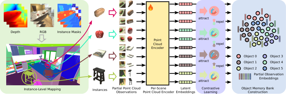
Depth back-projects each instance mask into 3D; camera poses transform observations into a global frame, and instance IDs determine which observations are fused. The resulting map supplies object labels for training. The main method description assumes known masks and odometry to isolate encoder performance, although the real-world experiments use estimated inputs. Reliable association within each exploration is therefore an upstream requirement rather than an outcome of the learned encoder.
IV-B Partial Point Cloud Observation Data Generation
Each reference mask yields a partial cloud of six-dimensional XYZ/RGB points in the camera frame. Subtracting the mean XYZ position centers the cloud: centered position equals original position minus the cloud centroid. The cloud and its map instance ID become a training example, and all views are retained. Centering gives translation invariance; it does not by itself remove viewpoint changes or arbitrary object rotations.
IV-C Training Scene-wise Object Point Cloud Encoder
Clouds larger than 1,024 points are voxel-downsampled at 1 cm and, if still too large, reduced by farthest-point sampling. Augmentation adds position jitter up to 3 cm and rotations from 0° to 30° about each axis. DGCNN uses ten neighbors; PointNet is the simpler alternative. An extra MLP projects the backbone embedding for the contrastive loss only. Inference uses the pre-projection embedding. Views with the same object ID are positives and views of other objects are negatives.
A batch starts with 64 random examples and adds one positive for each, giving 128 samples. Training uses learning rate 0.003 for 300 epochs, a 90/10 training/validation split, and checkpoint selection by validation loss evaluated every 300 iterations. The retained equation is the published NT-Xent-style objective. Its notation does not explicitly define the similarity inside the exponential, and the printed numerator/denominator place temperature differently; the equation is preserved without silently treating that typography as a fully specified implementation.

Equation 1
| (1) |
IV-D Object Memory Bank Generation
After training, every partial reference cloud is embedded and stored with its object ID. Multiple observations of one object occupy multiple memory entries, allowing a new partial view to retrieve similar past views. This is not a single prototype per object. Storage grows with reference observations, and the procedure trains a new encoder for each scene rather than establishing zero-shot transfer to unseen scenes.
IV-E Object Association in Dynamic Environment
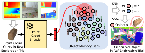
A new mask is back-projected, centered, voxel-downsampled, and encoded. Its ten closest stored embeddings vote for reference IDs. Votes accumulate across observations sharing a new-trial instance ID; a candidate’s score is its vote count divided by the total votes for that new object. These frequencies are called probabilities, but are not calibrated uncertainty estimates and may aggregate correlated views. Pure BYE independently chooses each object’s most frequent reference ID, which does not enforce the problem’s one-to-one mapping.
For ensembling, HOV-SG [20] builds a voxel feature map using CLIP [13]. For each object, nearby voxel features are collected, DBSCAN selects the dominant cluster, and the feature nearest its mean represents that object. Cosine similarity forms a visual-language score matrix. Adding it to normalized BYE vote scores and applying the Hungarian algorithm produces a bijection. Thus the ensemble changes both features and assignment rule relative to pure BYE. The small encoder is trained from scratch, while the ensemble still benefits from large-scale foundation-model pretraining.
V Experimental Results
Experiments compare object identity association in changed simulated scenes and two physical settings, then measure point-cloud preprocessing/encoding throughput.
V-A Object Association in Long-Term Dynamic Environments
Ten AI2-THOR reference scenes—five kitchens and five bedrooms—are manually explored and revisited after objects are relocated. Each scene gets its own encoder. The evaluation covers 252 movable object instances across 63 categories; fifteen frequent categories receive separate table columns. DINOv2, LSeg, OVSeg, and CLIP features are fused through the same voxel/object construction and matched with Hungarian assignment. Pure BYE uses majority assignment, so its comparison also differs in assignment constraints.
Overall success is 50.3% for DINOv2, 50.0% for LSeg, 75.4% for OVSeg, and 88.9% for CLIP. BYE alone reaches 82.9% with DGCNN and 85.7% with PointNet. Combining CLIP with these encoders reaches 92.5% and 95.6%, respectively: the best result improves over CLIP by 6.7 percentage points. The evidence favors complementarity, not universal superiority of the small encoder. Per-category results suggest gains for some small or less common objects, but several columns contain only four to six instances, and category rarity is not independently measured. Table I retains all category counts and scores.
| Method | Success Rate (%) | |||||||||||||||
|---|---|---|---|---|---|---|---|---|---|---|---|---|---|---|---|---|
| Overall | Garbage Can | Bowl | Mug | Cell Phone | Credit Card | Stool | Bread | Desk | Key Chain | Alarm Clock | Laptop | Pan | Pen | Salt Shaker | Spoon | |
| (252) | (10) | (9) | (9) | (6) | (6) | (6) | (5) | (5) | (5) | (5) | (5) | (5) | (5) | (5) | (4) | |
| DINOv2 [46] | 50.3 | 70 | 55.6 | 33.3 | 16.7 | 50 | 83.3 | 20 | 80 | 60 | 20 | 60 | 40 | 40 | 20 | 75 |
| LSeg [47] | 50.0 | 80 | 55.6 | 44.4 | 16.7 | 0 | 100 | 40 | 40 | 40 | 40 | 100 | 20 | 0 | 40 | 25 |
| OVSeg [14] | 75.4 | 100 | 77.8 | 77.8 | 50 | 50 | 100 | 60 | 80 | 60 | 60 | 100 | 40 | 60 | 40 | 75 |
| CLIP [13] | 88.9 | 100 | 100 | 88.9 | 83.3 | 100 | 100 | 100 | 100 | 100 | 80 | 100 | 80 | 20 | 40 | 50 |
| BYE (DGCNN) | 82.9 | 90 | 66.7 | 77.8 | 100 | 100 | 100 | 100 | 100 | 100 | 80 | 60 | 100 | 0 | 80 | 75 |
| BYE (PointNet) | 85.7 | 90 | 77.8 | 77.8 | 66.7 | 100 | 100 | 100 | 80 | 100 | 80 | 60 | 100 | 40 | 80 | 100 |
| BYE (DGCNN + CLIP) | 92.5 | 100 | 88.9 | 77.8 | 100 | 100 | 100 | 100 | 100 | 100 | 80 | 100 | 100 | 60 | 100 | 100 |
| BYE (PointNet + CLIP) | 95.6 | 100 | 88.9 | 100 | 100 | 100 | 100 | 100 | 100 | 100 | 80 | 100 | 100 | 80 | 100 | 100 |
The overall and per-class object association success rates in 10 AI2THOR scenes. The number in the parenthesis denotes the total occurrence number of a specific kind of object.
V-B Real-World Experiments
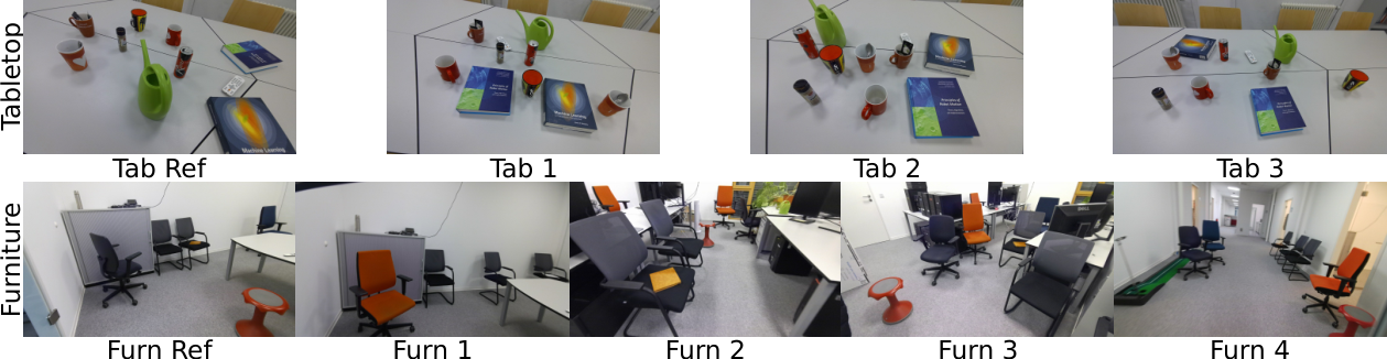
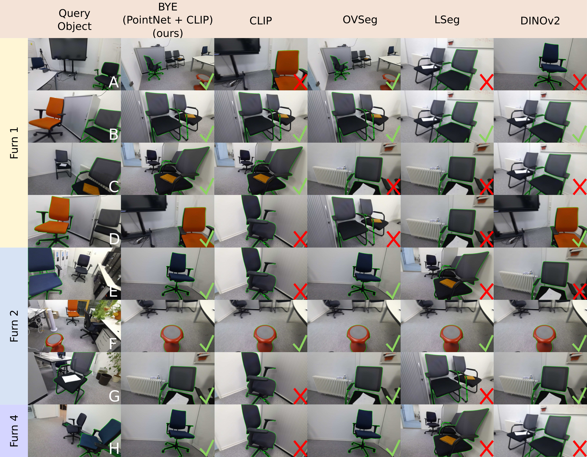
A tabletop setting contains ten objects in four layouts, and a furniture setting contains eight chairs across three rooms in five layouts. One exploration per setting trains the encoder; the other layouts test association, giving 30 tabletop and 32 furniture decisions. Chair-seat contents vary, including paper, notebooks, or empty seats. Azure Kinect supplies observations, SAM 2 supplies masks, and DROID-SLAM supplies poses; upstream errors are not separately quantified.
CLIP and both BYE backbones achieve perfect tabletop matching. Furniture is harder: CLIP ranges from 62.5% to 100%, DGCNN BYE from 87.5% to 100%, and PointNet BYE from 62.5% to 100%. Both ensembles achieve all 62 reported associations. The qualitative grid shows every compared method’s chair matches. This is a small, scene-adapted test rather than evidence of universal perfect accuracy or transfer without collecting a new scene’s training data.
| Method | Success Rate (%) | ||||||
|---|---|---|---|---|---|---|---|
| Tab 1 | Tab 2 | Tab 3 | Furn 1 | Furn 2 | Furn 3 | Furn 4 | |
| DINOv2 [46] | 40 | 40 | 40 | 37.5 | 25 | 37.5 | 50 |
| LSeg [47] | 40 | 40 | 40 | 25 | 12.5 | 25 | 25 |
| OVSeg [14] | 80 | 80 | 80 | 62.5 | 100 | 100 | 75 |
| CLIP [13] | 100 | 100 | 100 | 62.5 | 62.5 | 100 | 62.5 |
| BYE (DGCNN) | 100 | 100 | 100 | 100 | 87.5 | 87.5 | 87.5 |
| BYE (PointNet) | 100 | 100 | 100 | 75 | 100 | 100 | 62.5 |
| BYE (DGCNN + CLIP) | 100 | 100 | 100 | 100 | 100 | 100 | 100 |
| BYE (PointNet + CLIP) | 100 | 100 | 100 | 100 | 100 | 100 | 100 |
V-C Runtime Analysis
Timing uses a Ryzen 9 PRO 7945, RTX 4060 Ti with 16 GB memory, one CPU loading thread, and 41,267 partial clouds. It includes downsampling and encoding. At batch size one, the table reports 16.7 ms per cloud for DGCNN and 19.7 ms for PointNet; at batch size 32, amortized costs are 11.3 and 11.5 ms, or about 88.5 and 87 clouds/s. These are throughput measurements, not complete online mapping latency: segmentation, SLAM, foundation features, training, memory retrieval, and assignment are not included. Training duration and memory-bank storage cost are not reported.
VI Conclusion
BYE’s useful contribution is scene-specific identity learning from one exploration, particularly when combined with general visual-language features. Limits include dependence on instance-mask supervision, one encoder per scene, static objects within trials, unsupported additions/removals, and a small physical evaluation. The matching-rule difference also complicates isolating the ensemble’s feature benefit. Integrating the representation into open-vocabulary maps, real navigation, and lifelong learning is future work, not an evaluated capability.