At a glance
A nonlinear coordinate system can make collision-free planning regions convex while distorting the distance a robot actually travels. This paper refines an existing graph-of-convex-sets solution with a nonconvex cost evaluated in the original configuration space. Projected gradient steps retain the same convex feasibility constraints and discrete region sequence.
The reported benefits depend on the domain: bimanual paths average 20.60% shorter and 31.02% faster after retiming; Euler-angle plans reduce relative rotational-distance error by 42.5%; rational-coordinate examples show smaller average gains. The refinement preserves the supplied corridor’s feasibility, but does not certify a global optimum of the new objective.
I Introduction
Optimization-based planning can express smoothness, collision avoidance, and coordinated-arm constraints, but a general nonconvex formulation may fail locally. GCS trajectory optimization instead represents free space by a union of convex regions, with discrete decisions choosing which regions a continuous path traverses.
Some useful regions exist only after changing coordinates: inverse kinematics can eliminate a bimanual loop constraint, Euler angles represent rotations, and tangent half-angle coordinates permit algebraic collision certificates. Euclidean distance in these coordinates can be a poor proxy for joint motion or rotational distance.
The proposed postprocessor keeps the region sequence and convex constraints, but measures motion after mapping back to the physical configuration representation. It also tests a curvature cost to trade path length for faster acceleration-limited traversal. This adds modeling flexibility within the selected corridor; it does not revisit the discrete route or inherit global optimality for the new nonconvex cost.
II Background and Related Work
Sampling methods approximate free space effectively, while trajectory optimization handles richer objectives and constraints. Methods such as CHOMP, STOMP, and cuRobo manage nonconvexity through initialization, stochasticity, or parallel local solves. The present approach isolates nonconvexity in the objective after constructing a convex feasible corridor.
II-A Graphs of Convex Sets
A GCS vertex contains continuous variables in a convex set, and graph edges connect compatible regions. Bézier control points describe a path segment within each region; the convex-hull property keeps the entire segment inside it. Continuity and differentiability constraints can also remain convex.
The initial convex objective sums distances between adjacent control points, a proxy for curve length. The refinement keeps spatial planning separate from time allocation and uses TOPP-RA to retime the resulting path under motion limits. This avoids introducing acceleration/time-scaling nonconvexity into the projection constraints. Feasibility depends on valid regions, coordinate maps, and the retiming problem’s assumptions.
II-B Parametrizing Configuration Space
Three coordinate constructions motivate correcting the objective while retaining the planning constraints.
II-B 1 IK and Constrained Bimanual Planning
For two seven-joint arms holding a fixed relative end-effector transform, analytic inverse kinematics derives the subordinate arm from the leading arm and a redundancy coordinate. The planning representation has eight dimensions instead of the full fourteen. A short path there can neglect substantial motion by the subordinate arm.
II-B 2 Euler Angles and GCS on SO ( 3 )
Euler-angle coordinates simplify the convex-region construction for 3D rotations, but their Euclidean distance does not reproduce the rotation group’s geometry and becomes poorly behaved near coordinate singularities. Quaternion and axis-angle baselines use piecewise-linear representations with their own approximation and planning costs.
II-B 3 Rational Kinematics to Certify Collision Free
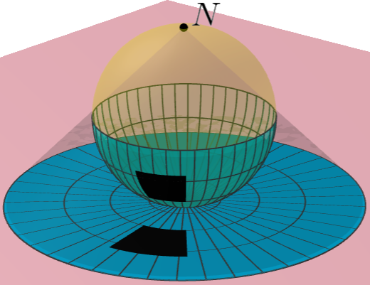
The substitution s = tan(θ/2) makes trigonometric kinematics rational, enabling semidefinite certificates for collision-free regions or trajectories. The inverse map is θ = 2 arctan(s). Near θ = ±π, small angular changes can occupy very large coordinate distances, biasing a convex distance objective toward the nominal pose.
The source’s displayed sine/cosine identities contain errors. For this substitution the correct identities are sin(θ) = 2s/(1+s²) and cos(θ) = (1−s²)/(1+s²). The original display is retained below for fidelity; the method’s inverse-coordinate map and the distortion argument use the stated tangent substitution.
Equation
II-C Nonconvexity and GCS
Existing approaches use hand-designed convex surrogate costs, piecewise convex approximations, or special alternating formulations. This method instead evaluates a nonlinear objective directly and projects only against convex constraints.
Keeping nonconvex constraints outside the refinement is a deliberate restriction. The method does not solve arbitrary nonlinear dynamics or acceleration constraints within GCS; it handles timing separately and improves a fixed feasible spatial path.
III Methodology
The optimizer changes how path quality is measured while retaining the original convex feasible set for its control points.
III-A Nonlinear Changes of Coordinates
A smooth map α takes a point in the useful planning coordinates to the original configuration representation. For bimanual motion it reconstructs all fourteen joints; for Euler angles it produces a quaternion; for rational coordinates it applies twice the arctangent. The cost uses α, while region membership remains in the planning coordinates.
III-B Formulating the Optimization
Transforming Bézier control points does not generally transform the whole Bézier curve correctly. The method therefore samples each curve segment in planning coordinates, maps those actual curve points through α, and evaluates distances between successive transformed samples.
The experiments use ten samples per region and sum squared segment distances. Bimanual and rational cases use Euclidean joint-space distances; rotations use the spherical interpolation distance. This is a discretized energy-like proxy for length, not exact continuous arc length. Its relationship to length also depends on sampling and parameterization, so finite-sample improvements must be measured on the resulting path.
The retained optimization displays contrast the original control-polygon cost with the mapped-sample cost. Both use the same region sequence and convex control-point constraints; only the objective changes.
Equations
III-C Projected Gradient Descent
Each projected gradient iteration takes a descent step, then returns the control points to the feasible polyhedron. Full projection is a convex quadratic program solved with Mosek. A feasible starting path ensures the fixed corridor is nonempty, and exact projection preserves its constraints.
The source’s convergence wording is stronger than justified: a Lipschitz objective alone does not guarantee a local minimum, and standard smooth-gradient step conditions involve the inverse of a gradient Lipschitz constant. Nonconvex projected gradient methods generally target stationary points under suitable assumptions. The authors do not establish such a constant for these objectives; the experiments use backtracking and a finite stopping rule.
III-D Solver Performance
Initialization, step selection, compiled gradients, cheaper projections, and termination criteria determine the practical overhead.
III-D 1 Initialization
The implementation refines the best rounded GCS solution, preserving its discrete path. Running the refinement on several candidate paths during rounding is proposed as an extension. Local results remain dependent on the starting path and corridor.
III-D 2 Optimal Step Sizes
Backtracking repeatedly halves a candidate step until an Armijo sufficient-decrease condition is met. This avoids choosing one fixed step manually; it does not find a globally optimal step or eliminate local stationary points.
III-D 3 Gradient Precompilation
JAX precompiles gradients for individual vertices so they can be reused across start–goal queries. The reported online refinement time therefore excludes this offline compilation work.
III-D 4 Affine Projections
A cheap affine-hull projection first enforces equality constraints such as continuity. If the projected point also satisfies the inequalities, a full quadratic program is unnecessary. Otherwise the solver projects onto the entire feasible polyhedron. This shortcut is most useful for small or fixed steps.
III-D 5 Convergence Criteria
The solver stops when the change in a five-iteration moving-average cost falls below 0.5%, or after seventy iterations. These are practical stopping rules, not certificates of optimality. The authors note occasional cost jumps associated with projection and report that most converged cases finish well before the cap.
III-E More general nonconvex objectives: Curvature
A curvature penalty targets sharp bends that force slower traversal under acceleration limits. Curvature is evaluated at sampled points, and a smooth maximum approximates the worst value along the path. A weighted distance/curvature objective can produce a longer but faster trajectory after retiming.
The geometric curvature formula is retained. It is singular where the path derivative vanishes, another reason to distinguish a practical sampled implementation from an unrestricted smooth-objective guarantee.
Equation
IV Experiments
Every experiment first solves the original convex-surrogate GCS problem, then refines its rounded solution. Bimanual cases include hardware and simulation; rotation tests are abstract obstacle-free problems, and rational-kinematics tests are simulated.
IV-A Constrained Bimanual Motion Planning
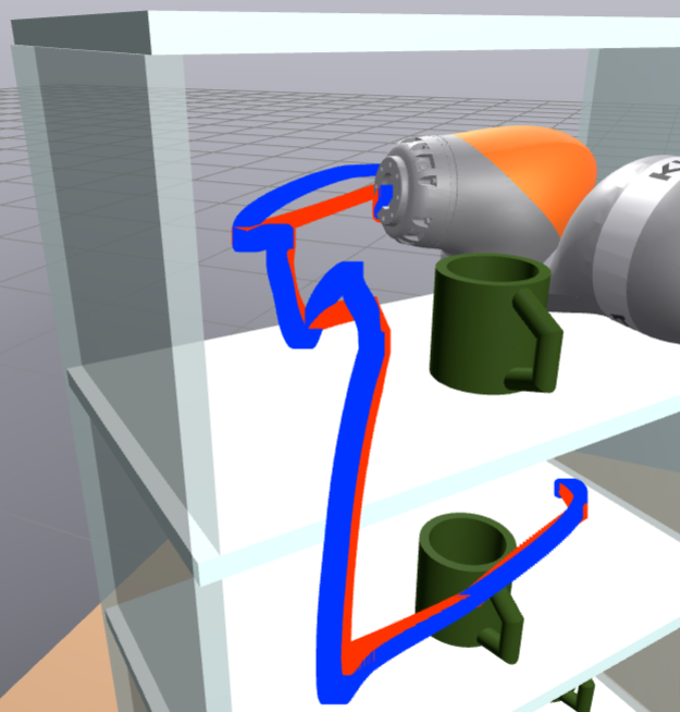
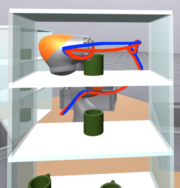
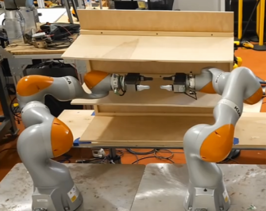
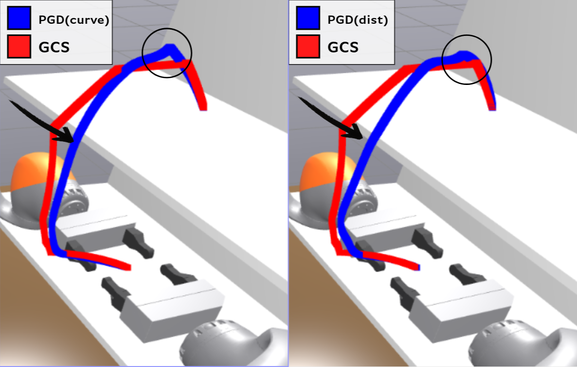
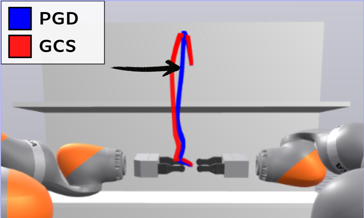
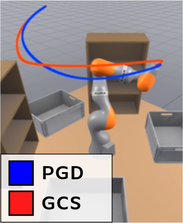
Two iiwa arms move among shelves while maintaining a fixed relative end-effector transform. Table I compares the original eight-dimensional surrogate, full fourteen-joint distance, and a manually weighted distance/curvature combination on three benchmark routes.
For top-to-bottom motion, distance refinement reduces length from 5.622 to 5.048 and duration from 7.48 to 4.263 seconds. Adding curvature gives a slightly longer 5.13 path but a shorter 3.99-second traversal. The same tradeoff appears on the other two routes. The complete table retains all durations, lengths, and imbalance values.
Imbalance is (subordinate-arm distance − leading-arm distance) divided by their sum. Distance refinement moves it closer to zero; curvature regularization sacrifices some of that balance. Across 100 randomly sampled start/goal configurations, paths average 20.60% shorter and 31.02% faster. Refinement averages 0.0554 seconds and 13.7 iterations beyond 2.133 seconds for the original optimization.
About 80% of refinement time goes to quadratic-program projections. With backtracking, the affine-hull shortcut is almost never sufficient: gradients tend to push outward against active collision boundaries. The authors suggest same-handed arm geometry as a possible explanation for residual imbalance, rather than establishing it experimentally.
Equation
| Top to Middle | |||
| GCS | Distance | Distance + Curvature | |
| Trajectory Time | 4.889 | 3.469 | 3.243 |
| R14 Path Length | 4.241 | 3.766 | 3.884 |
| Imbalance | 0.331 | 0.117 | 0.216 |
| Middle to Bottom | |||
| GCS | Distance | Distance + Curvature | |
| Trajectory Time | 5.326 | 3.08 | 2.99 |
| R14 Path Length | 3.325 | 3.175 | 3.247 |
| Imbalance | 0.162 | 0.099 | 0.110 |
| Top to Bottom | |||
| GCS | Distance | Distance + Curvature | |
| Trajectory Time | 7.48 | 4.263 | 3.99 |
| R14 Path Length | 5.622 | 5.048 | 5.13 |
| Imbalance | 0.190 | 0.084 | 0.122 |
IV-B Planning over SO ( 3 )
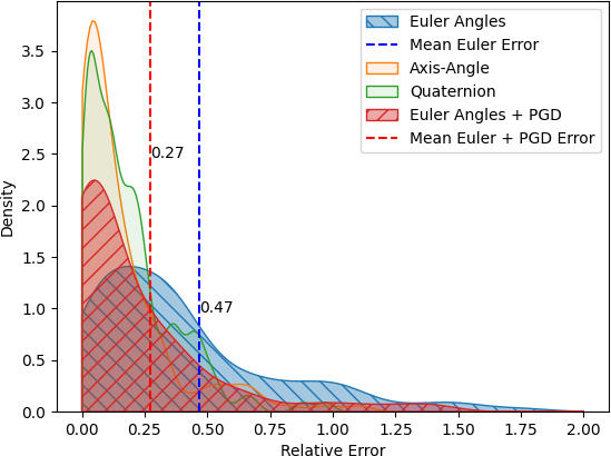
For 125 random rotation pairs without obstacles, spherical interpolation supplies the exact shortest rotational distance. Refinement starts from Euler-angle GCS paths; quaternion and axis-angle plans are comparison representations.
The reported average reduction is 42.5% in relative error against the shortest distance. Figure 5’s means shift from roughly 0.47 to 0.27. This is not a 42.5% reduction in path length; the discussion’s statement of approximately 40% shorter paths conflates the two metrics. Some paths improve little, possibly because a better discrete route lies outside the fixed corridor.
Refinement adds 4.08 seconds to the Euler solution’s 17.28 seconds: 0.62 seconds in the solver and 3.46 rebuilding/reusing the path representation. Axis-angle planning takes 41.10 seconds; low-resolution quaternion planning takes 16.73 seconds, while higher-resolution quaternion cases take minutes. Thus refined Euler planning is not faster than every quaternion setting.
IV-C Rational Parametrizations of Robot Kinematics
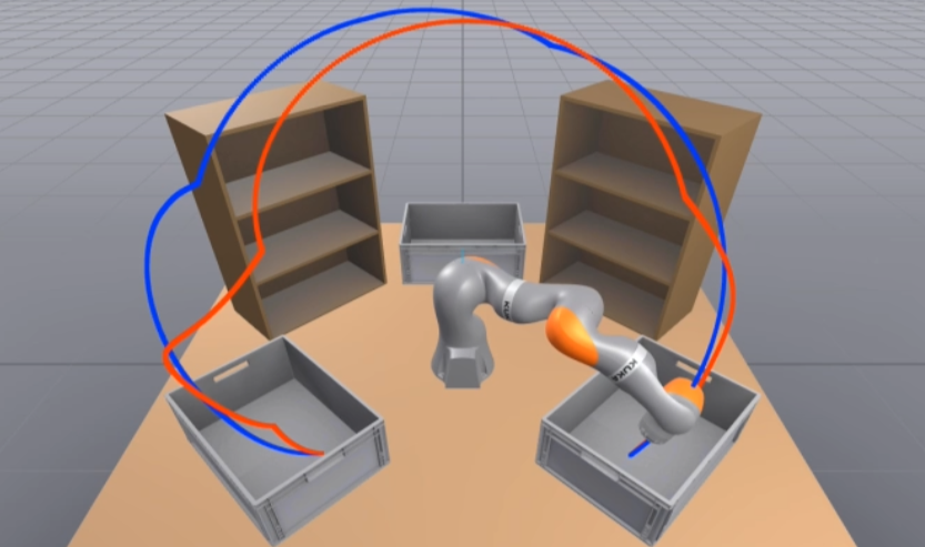
Rational-coordinate tests use a planar three-joint iiwa and a full seven-joint iiwa. Certified IRIS supplies collision-free regions for the planar case; the seven-joint trajectories admit the cited trajectory-certification procedure. The nominal pose has all joint angles zero.
Across 100 planar start/goal samples, average length improvement is only 0.2%; most runs stop within seven iterations and 0.22 seconds. The illustrated planar example improves by 1.2%. These small averages are consistent with mild distortion away from the tangent-coordinate limits.
For seven-joint bin-to-bin paths, average length and duration reductions are 3.89% and 4.74%. One illustrated path improves by 10.8% and 17.6%, respectively. Large gains are examples near more strongly distorted configurations, not the average performance of rational-coordinate planning.
V Discussion
The approach improves a chosen GCS corridor by evaluating costs in more meaningful coordinates, while convex projection maintains the modeled feasibility conditions. The biggest average gains occur in bimanual planning; rational-coordinate certification remains useful despite relatively small average distortion penalties.
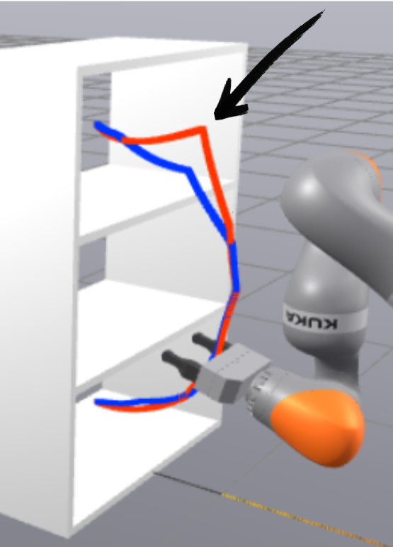
Added runtime, offline gradient compilation, fixed discrete routes, sampled costs, and local optimization limit the result. Sparse environments leave more room for refinement. The cluttered example shows improvement in a large region and little change in narrow regions; it does not establish a uniform improvement in dense clutter.
Future directions include parallel refinement during rounding, anytime planning, integration with GCS* or multi-query search, and better convex surrogate objectives. The surrogate still matters because it chooses the initialization and discrete corridor that this postprocessor cannot escape.