At a glance
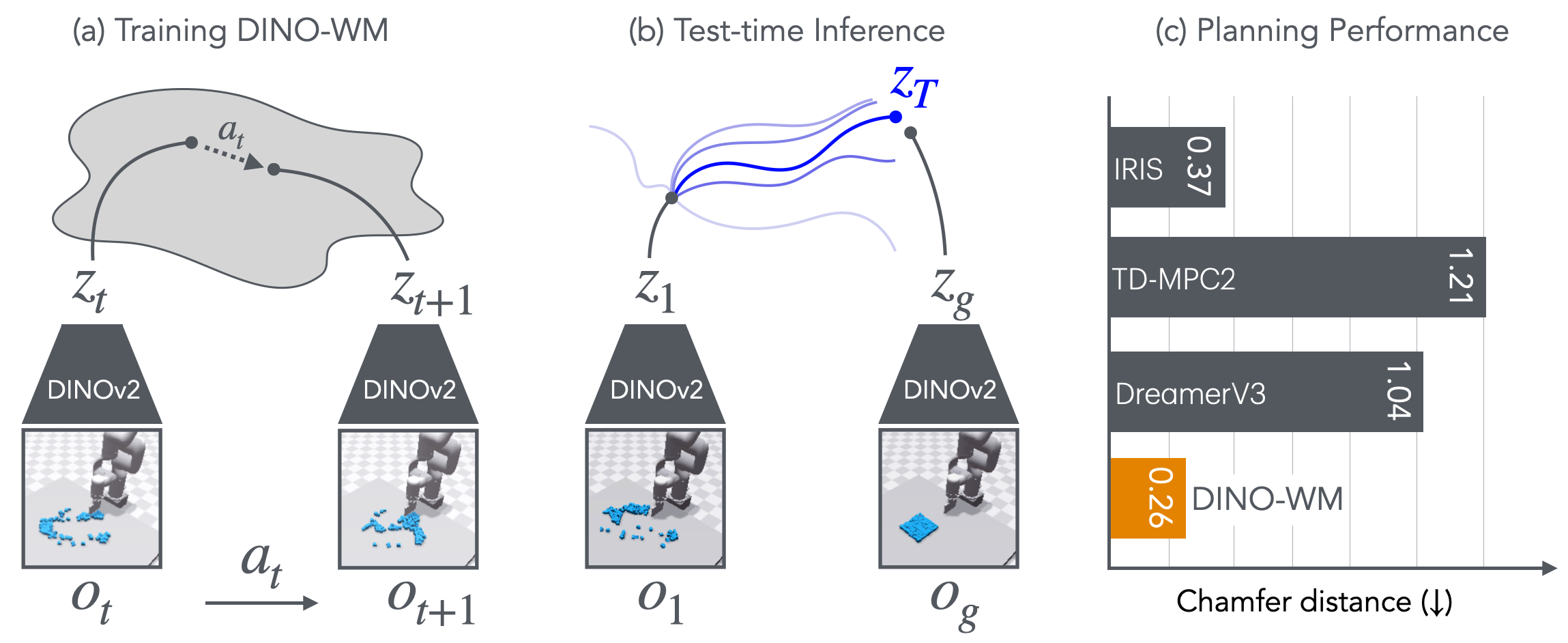
Intuition: learn a cheap simulator for what a camera sees, then try possible action sequences inside it before moving. DINO-WM freezes a pretrained DINOv2 image encoder and trains a predictor of its spatial patch features on recorded observation–action trajectories. A planner searches for actions whose predicted final features resemble a supplied goal image. Across six simulated environment suites, patch features support stronger manipulation and generalization than the tested global image representations. Zero-shot here means selecting new goals without training a task-specific policy; the dynamics model still learns from action-labeled data for the environment family. The experiments do not establish unrestricted real-world transfer or that visual similarity always defines the correct control objective.
1 Introduction
A policy stores an action-selection rule, while a predictive model can evaluate a fresh plan at deployment. The paper targets the latter using offline data. Its practical bet is that large-scale image pretraining supplies useful perception before dynamics training starts. Separating perception, future prediction and planning makes new visual goals possible without a new reward model. Generalization still depends on the offline data covering relevant interactions.
2 Related Work
The closest context is visual model-based control, video generation and pretrained visual representations. DINO-WM predicts useful image features rather than generating pixels during planning. This removes a decoder from the control loop, but inherits the encoder’s blind spots. Comparisons with reward-based systems modify their original objectives to fit the reward-free setting, so they compare these adaptations rather than each baseline at its intended best use.
3 DINO World Models
The input is a current camera observation, recent observations and actions, and a target image. The objective is to reach a physical state that looks like that target. Partial observability motivates temporal context: one image may reveal position without revealing velocity. The proposed representation and planner are described separately below.
3.1 DINO-based World Models ( DINO-WM )
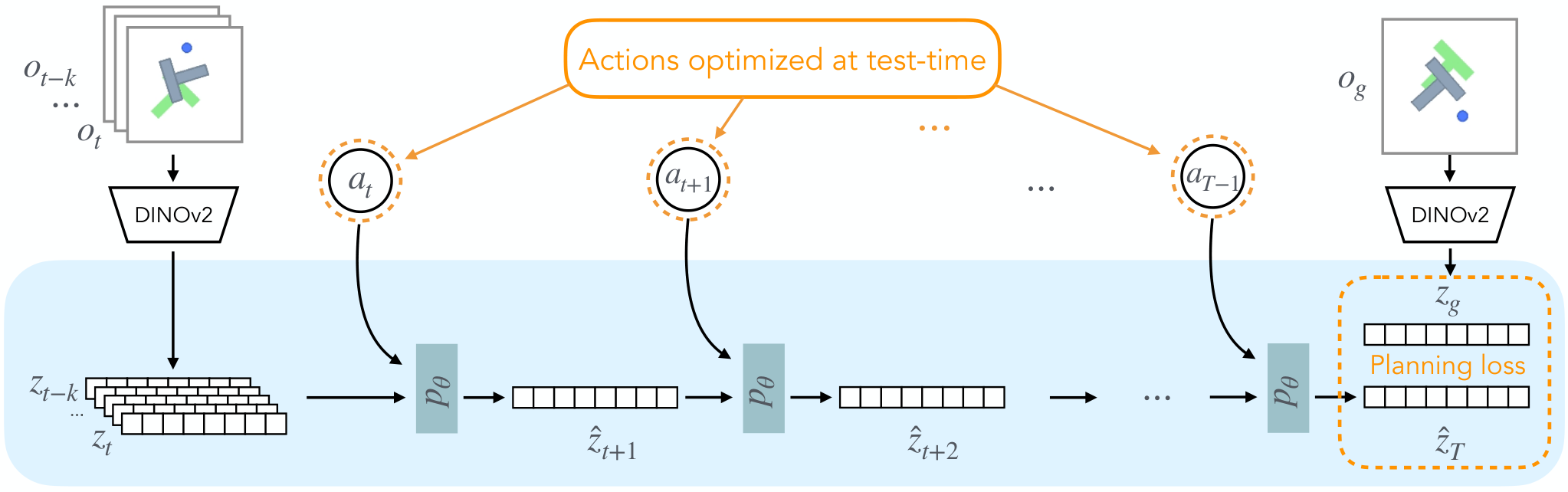
Three modules have distinct jobs: a frozen encoder extracts spatial features, a learned action-conditioned model predicts their evolution, and an optional decoder converts features back to images for inspection. Only the first two are needed for planning. Training the decoder separately prevents its reconstruction objective from changing the predictive representation.
Equation
| Observation model: | |||
| Transition model: | |||
| Decoder model: | |||
| (optional for visualization) |
3.1.1 Observation Model
DINOv2 produces a grid of patch vectors, retaining where things appear in the scene. Its parameters remain fixed during both training and deployment. This supplies a stable prediction target and useful image semantics, while avoiding collapse caused by a jointly learned encoder returning a constant. It does not guarantee that every hidden physical property is represented.
3.1.2 Transition Model
The predictor consumes recent patch grids plus embedded actions and, where available, proprioception. A transformer predicts the next entire grid. Its causal attention mask permits only earlier frames as evidence; all patches of the next frame are predicted together. Training uses real previous observations as context, a procedure called teacher forcing, and minimizes squared error to the frozen encoder’s next-frame features. At planning time, later inputs are the model’s own predictions, so errors can accumulate.
Equation 1
| (1) |
3.1.3 Decoder for Interpretability
The optional decoder learns to reconstruct images from encoded features. It is a diagnostic for inspecting predicted object positions and motions, not a requirement for choosing actions. A plausible decoded frame can help spot failures, but visual quality alone does not establish correct dynamics or successful control.
Equation 2
| (2) |
3.2 Visual Planning with DINO-WM
Encode the current and goal images, simulate candidate actions, and minimize the final latent distance to the goal. The cross-entropy method repeatedly samples action sequences, keeps the best ones and refits their sampling distribution. Model predictive control executes only a prefix and replans after receiving new observations. Gradient descent through the differentiable predictor is possible, but performs worse in the reported comparison; differentiability alone does not make this search easy.
Equation
4 Experiments
The evaluation asks whether offline training yields usable dynamics, whether those dynamics support planning, how much the encoder matters, and whether performance transfers to changed configurations. All six suites are simulated. The control metric differs between rigid navigation/manipulation and deformable objects.
4.1 Environments and Tasks
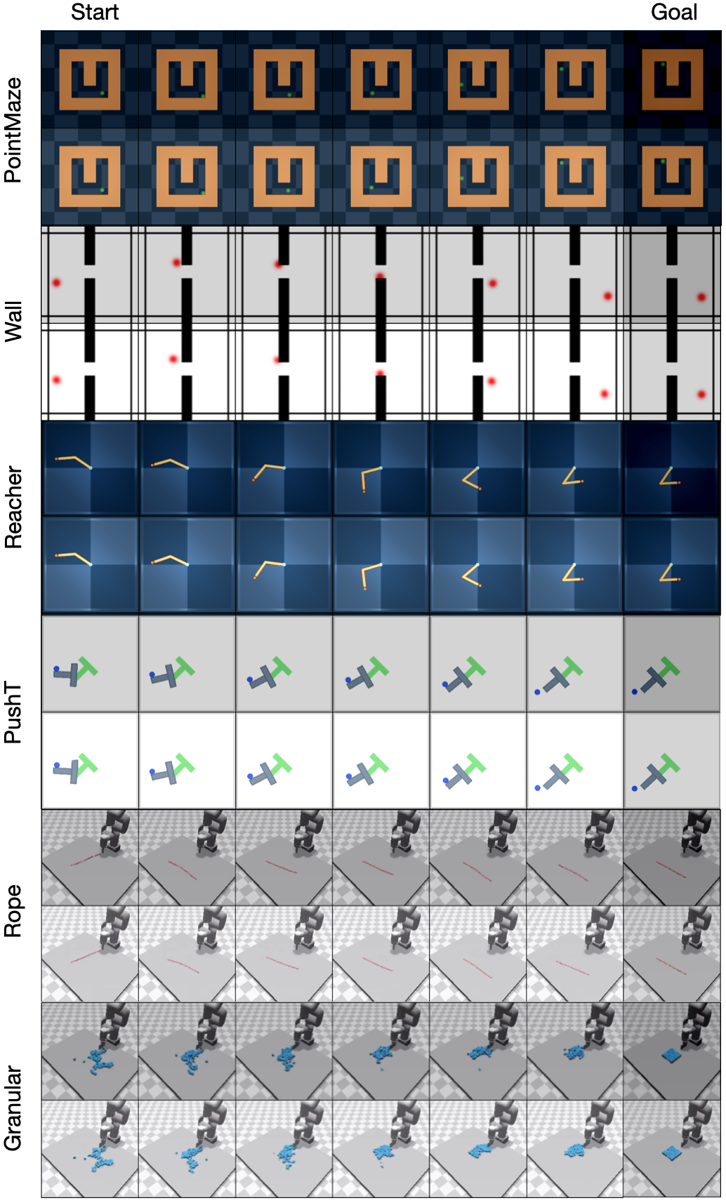
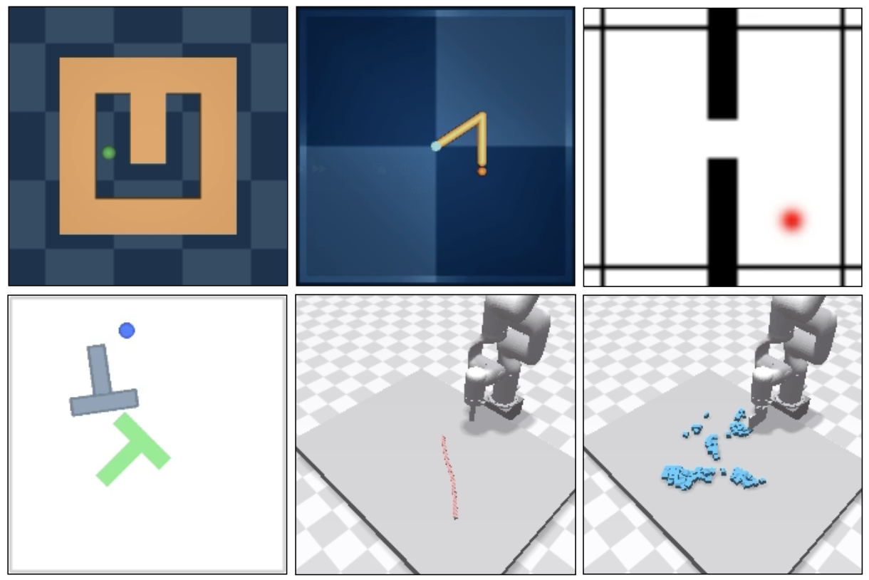
The suites cover maze navigation, a two-room wall, arm reaching, pushing a T-shaped block, moving a rope and gathering particles. A target image specifies each task. Feasible Push-T goals are selected within a short horizon; this is a bounded goal-reaching problem rather than arbitrary long-horizon manipulation.
4.2 Baselines
IRIS, DreamerV3 and TD-MPC2 are adapted to train offline without their usual reward information, then used with planning. An action-conditioned AVDC video generator supplies another comparison. Reward removal is a substantial change for methods whose representations normally depend on rewards. Their poor performance here should not be read as a general ranking of the original algorithms.
4.3 Optimizing Behaviors with DINO-WM
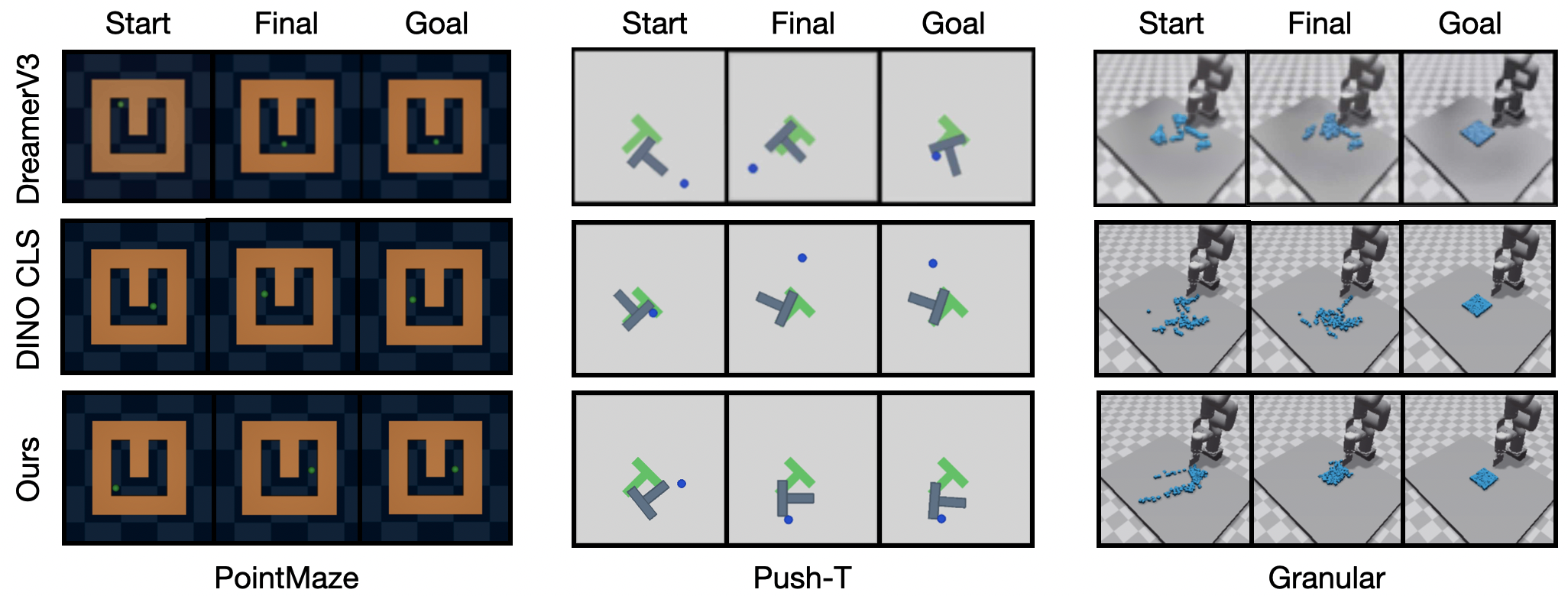
DINO-WM is strong on reaching and manipulation, while DreamerV3 slightly exceeds it on the two easiest navigation settings. Success rates use fifty start–goal pairs; rope and granular tasks instead report Chamfer distance over ten instances. Lower Chamfer distance means the final point configurations are closer. These distances cannot be compared numerically with success percentages.
4.4 Does pre-trained visual representations matter?
Replacing patch features with R3M, ImageNet ResNet or DINO’s single global token hurts several spatially precise tasks. The controlled comparison supports retaining local spatial information. It does not isolate patch structure from every pretraining or architecture difference among all encoders.
4.5 Generalizing to Novel Environment Configurations
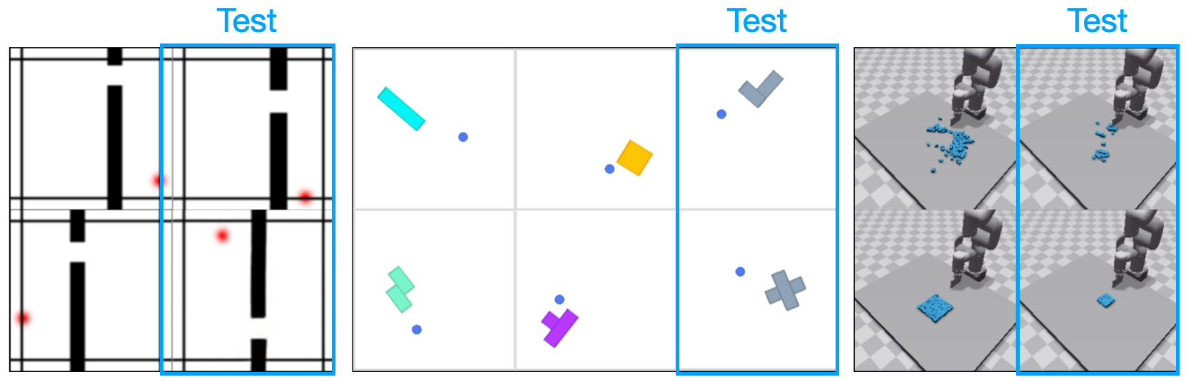
Held-out wall and door positions, unseen block shapes and changed particle counts test transfer within related environment families. DINO-WM leads the compared methods, but PushObj success is only 34%: unfamiliar contact geometry remains difficult. The explanation that patch features tolerate particle-count changes is a plausible interpretation rather than an independently verified mechanism.
4.6 Qualitative comparisons with generative video models
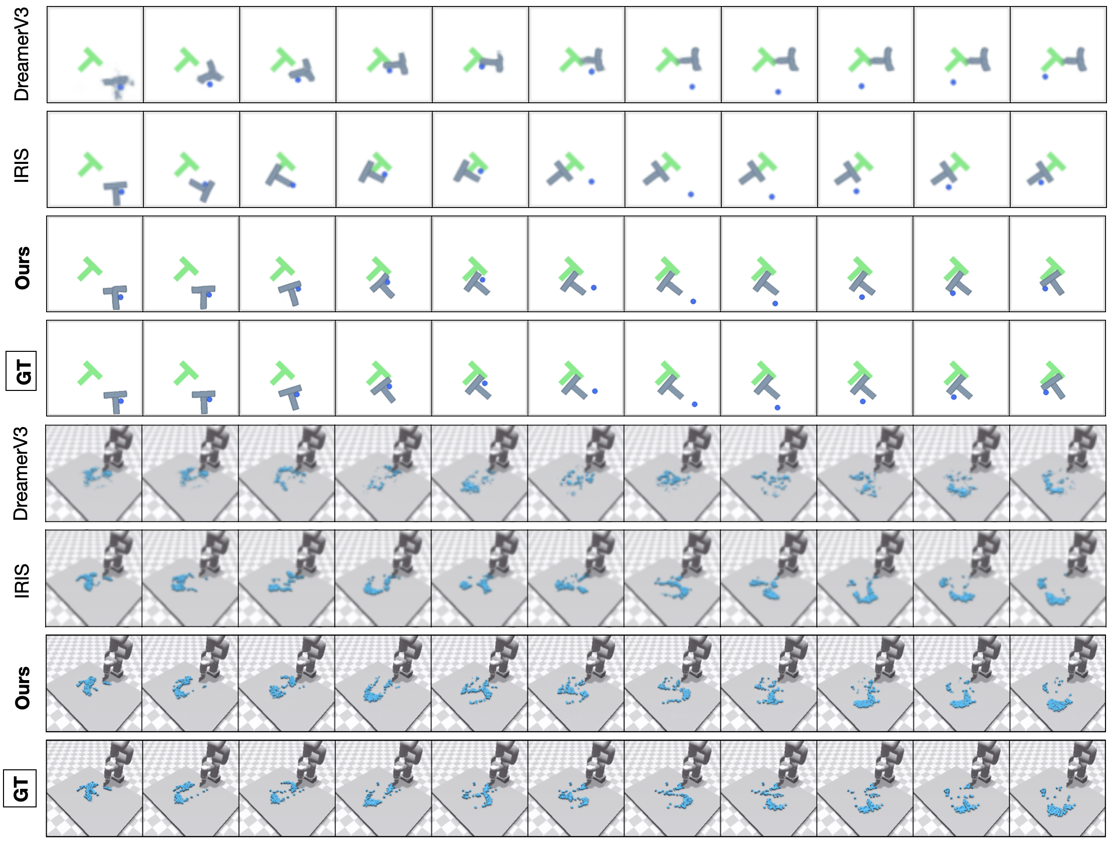
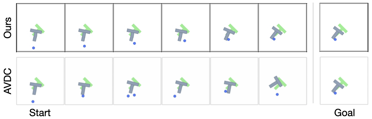
Selected AVDC generations can look realistic while violating the action-conditioned physical trajectory. The additional action-conditioned comparison also shows long-rollout divergence. These examples distinguish visual plausibility from control usefulness; they do not prove that every generative world model must fail.
4.7 Decoding and Interpreting the Latents
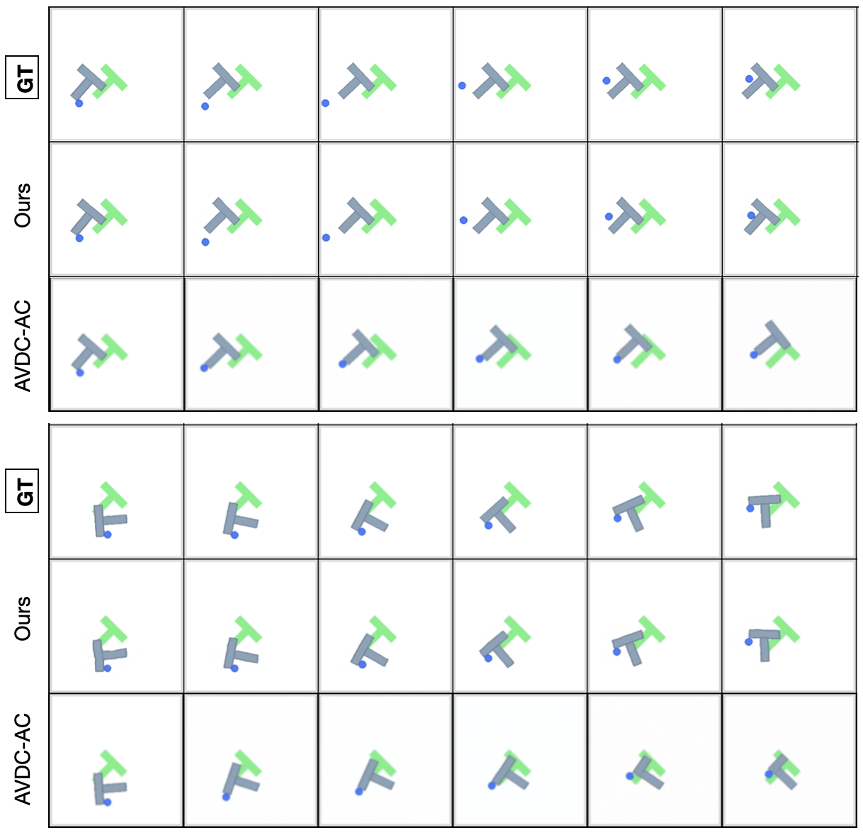
A separately trained decoder lets the authors measure image-space agreement after latent prediction. Lower LPIPS and higher SSIM indicate better decoded perceptual and structural similarity. These are auxiliary diagnostics; the planning results remain the direct test of whether predicted features support behavior.
5 Conclusion
The contribution is a simple frozen-feature dynamics pipeline that supports planning without reward labels or a learned task policy. Its main dependencies are sufficient state–action coverage, recorded action labels and a useful visual goal representation. Broader real-world deployment, learning from videos without actions and hierarchical long-horizon control remain future directions.
Impact Statement
The authors identify general advances in machine learning and do not discuss application-specific societal impacts in detail.
Acknowledgements
The source acknowledges research discussions, institutional grants and fellowship support.
Appendix A Appendix
A.1 Environments and Dataset Generation
Dataset construction differs by task. Several navigation, arm and deformable-object datasets use random actions; Push-T includes noisy replays of expert trajectories. Thus the broad claim of not requiring expert demonstrations does not mean that no evaluated dataset contains expert-derived behavior. The suite also uses different success conditions and trajectory lengths, all retained in the source details.
A.2 Environment families for testing generalization
Generalization tests alter door positions, replace training block shapes with held-out shapes, or change the quantity and arrangement of particles. They test specified shifts within these families. No result here demonstrates transfer to an unrelated control system.
A.3 Pretraining features
R3M and ImageNet encoders provide global ResNet representations, while DINO CLS uses DINOv2’s global token. They form the comparison against its patch grid. Keeping this distinction clear explains why a strong image descriptor can still discard detail needed for contact control.
A.4 Ablations
A.4.1 Scaling Laws of DINO-WM
Increasing Push-T data from 200 to 18,500 trajectories improves both planning success and decoded prediction metrics. This is an empirical data-size trend within one setup, not a fitted universal scaling law. Small datasets remain a major limitation.
| Dataset Size | SR | SSIM | LPIPS | |
|---|---|---|---|---|
| n=200 | 0.08 | 0.949 | 0.056 | |
| n=1000 | 0.48 | 0.973 | 0.013 | |
| n=5000 | 0.72 | 0.981 | 0.007 | |
| n=10000 | 0.88 | 0.984 | 0.006 | |
| n=18500 | 0.92 | 0.987 | 0.005 |
A.4.2 DINO-WM with vs. without Causal Attention Mask
Without a temporal causal mask, a multi-frame training input can reveal the frame the model is supposed to predict. Training then becomes easier in a way unavailable during rollout. The mask prevents this shortcut: increasing history helps the masked model while strongly hurting the unmasked one. At history length one, the two constructions coincide.
A.4.3 DINO-WM with Reconstruction Loss
Backpropagating a pixel reconstruction loss through the predictor lowers reported Push-T success from 92% to 80%. The experiment favors separate decoder training in this setting. It does not establish that every reconstruction objective is harmful for all world models.
A.5 Planning Optimization
The appendix makes the planning procedures explicit and compares executing a complete optimized plan with replanning from new observations.
A.5.1 Model Predictive Control with Cross-Entropy Method
CEM scores many sampled action sequences by their predicted final goal error. It updates a Gaussian proposal using the best candidates, repeats for a fixed budget, executes a chosen prefix and starts again from the new observation. Replanning corrects some prediction and execution errors; it cannot repair an encoder or dynamics model that misses a crucial interaction.
Equations 3–5
| (3) |
| (4) |
| (5) |
A.5.2 Gradient Descent:
Gradient descent changes each proposed action using the derivative of final goal error through the predicted rollout. This trades large candidate populations for sensitivity to the loss landscape and initialization. The same model and latent cost do not guarantee the same search quality.
Equations 6–8
| (6) |
| (7) |
| (8) |
A.5.3 Planning Results
The table distinguishes open-loop CEM, open-loop gradient descent and CEM inside model predictive control. Replanning improves the reported tasks. Rope and granular entries under MPC are Chamfer distances, inherited from their task metrics; they are not success rates despite sharing the comparison table.
A.6 Comparison with Action-Conditioned Generative Models
The action-conditioned AVDC variant predicts a next observation from the current observation and action. Its selected open-loop rollouts drift from the true sequence. This is a stronger control-oriented comparison than a text-only video generator, but remains a particular trained baseline.
A.7 Decoding the Latents: LPIPS and SSIM Metrics
SSIM measures structural image similarity and LPIPS measures distance between perceptual features. The reported decoded rollouts favor DINO-WM across these tasks. The decoder introduces its own approximation error, so these scores probe the combined prediction-and-decoding pipeline.
| LPIPS | SSIM | |||||||
|---|---|---|---|---|---|---|---|---|
| Method | PushT | Wall | Rope | Granular | PushT | Wall | Rope | Granular |
| R3M | 0.045 | 0.008 | 0.023 | 0.080 | 0.956 | 0.994 | 0.982 | 0.917 |
| ResNet | 0.063 | 0.002 | 0.025 | 0.080 | 0.950 | 0.996 | 0.980 | 0.915 |
| DINO CLS | 0.039 | 0.004 | 0.029 | 0.086 | 0.973 | 0.996 | 0.980 | 0.912 |
| AVDC | 0.046 | 0.030 | 0.060 | 0.106 | 0.959 | 0.983 | 0.979 | 0.909 |
| Ours | 0.007 | 0.0016 | 0.009 | 0.035 | 0.985 | 0.997 | 0.985 | 0.940 |
A.8 Inference Time
One forward pass and a complete plan have very different costs. The source reports 0.014 seconds for a batched inference step but 53 seconds for CEM planning with 100 samples and ten iterations on an A6000. Fast latent simulation therefore does not imply real-time replanning. The simulator timing uses a different batch size and should not be treated as an equal-work hardware benchmark.
| Metric | Time (s) |
|---|---|
| Inference (Batch 32) | 0.014 |
| Simulation Rollout (Batch 1) | 3.0 |
| Planning (CEM, 100x10) | 53.0 |
A.9 Hyperparameters and implementation
The predictor has roughly 19 million parameters and uses task-dependent frame skips to avoid learning only tiny visual changes. The prose describes 196-pixel encoder input, while its shared table lists image size 224; both printed details are retained rather than silently reconciled. Task-specific trajectory counts and lengths also deserve attention when reproducing the experiments.
| Frameskip | Dataset Size | Traj. Len. | ||
|---|---|---|---|---|
| PointMaze | 3 | 5 | 2000 | 100 |
| Reacher | 3 | 5 | 3000 | 100 |
| Push-T | 3 | 5 | 18500 | 100-300 |
| PushObj | 3 | 5 | 20000 | 100 |
| Wall | 1 | 5 | 1920 | 50 |
| WallRandom | 1 | 5 | 10240 | 50 |
| Rope | 1 | 1 | 1000 | 5 |
| Granular | 1 | 1 | 1000 | 5 |
A.10 Additional Planning Visualizations
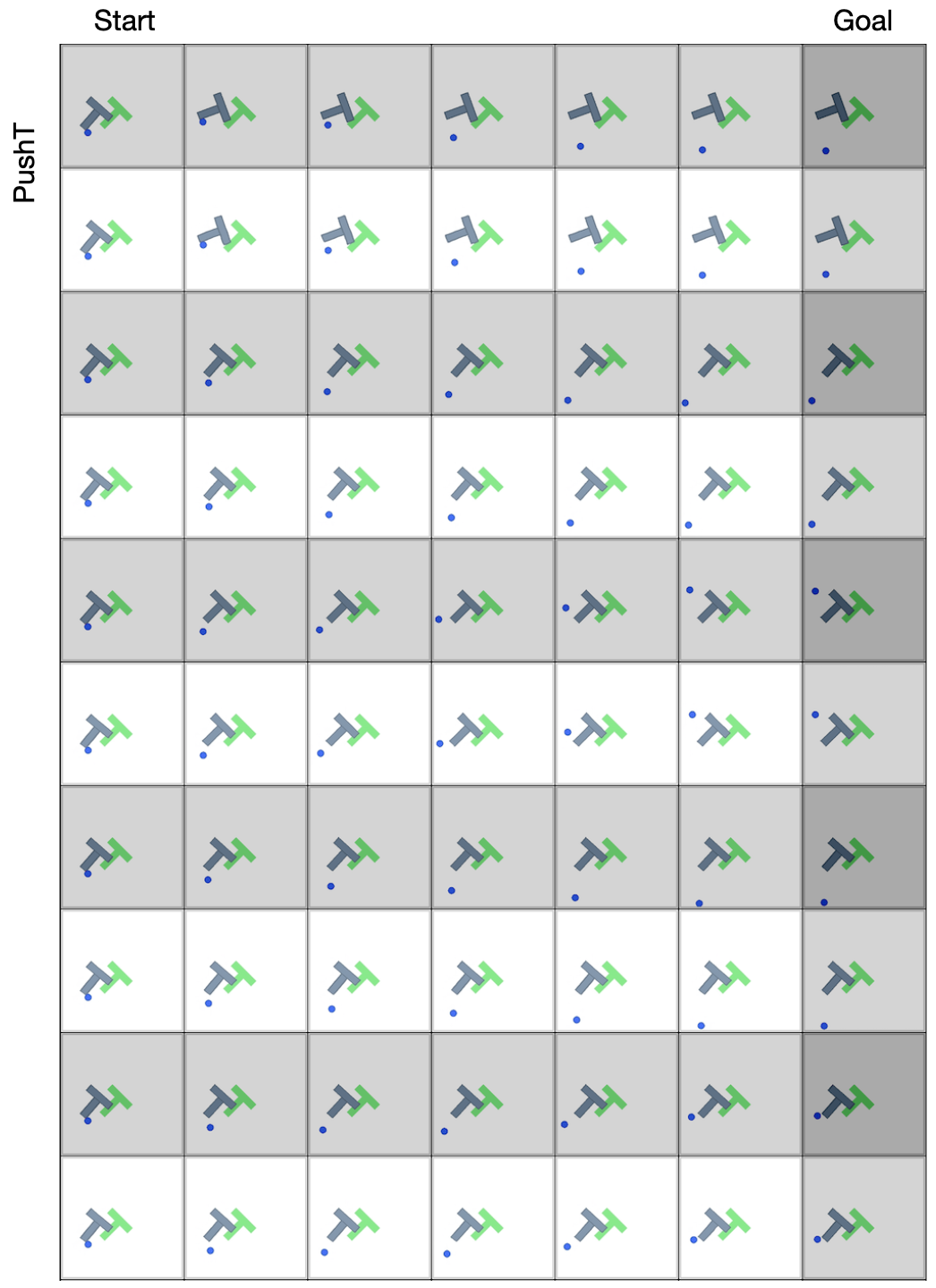
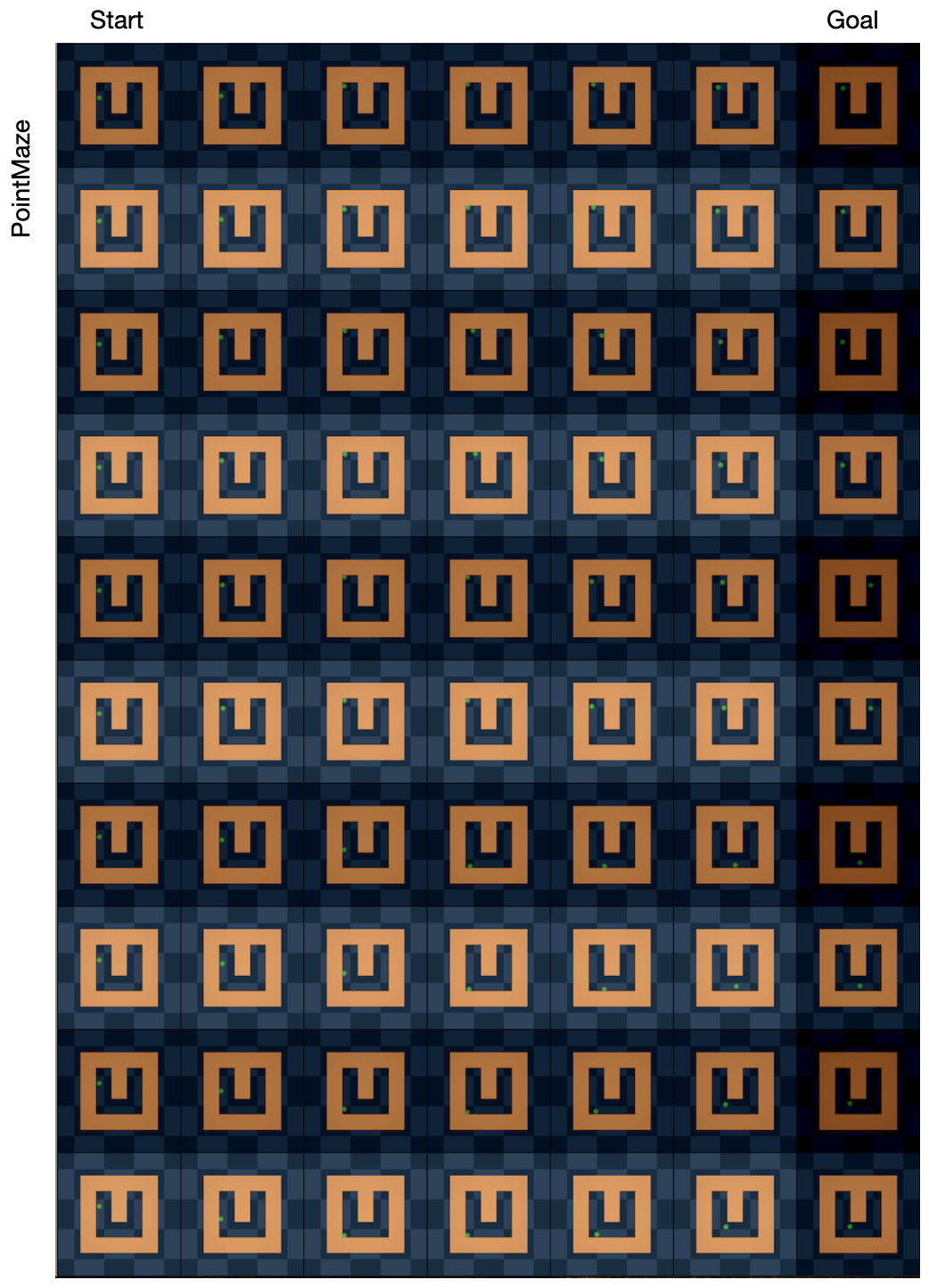
The final visualizations compare actual executed trajectories with decoded imagined trajectories and test different goals from the same initial state. They illustrate controllability and characteristic errors, while the quantitative evaluation determines how often those examples generalize.