A single layer of multi-head linear attention, without softmax, is a cubic polynomial in its input. The paper learns it by linear regression in a lifted feature space, then factorizes the fitted matrix into at most d² attention heads. This removes a rank constraint by allowing more heads; it does not solve the optimization problem for an arbitrarily fixed small number of heads.
A positive-definite second-moment matrix of reduced input features certifies that empirical minimizers represent the same function, under the stated realizability or width conditions. The paper applies this to bounded-history Turing-machine simulation and tests synthetic attention, associative memory, and finite-automaton execution. The polynomial-time construction is distinct from the stochastic-gradient optimizers used in most experiments.
1 Introduction
Expressing a computation with a Transformer does not show that its parameters can be learned efficiently from examples. This paper separates three questions: finding an empirical optimum, generalizing on a data distribution, and identifying the actual function strongly enough to generalize outside that distribution.
The algebraic observation is that products of value and key-query parameters can be collected into a d²-by-d² matrix. Relaxing its rank constraint gives ordinary least squares; singular-value decomposition converts the result back into an attention model. The method concerns one unnormalized linear-attention layer, even though related architectures motivate the introduction.
The identifiability certificate asks whether the training inputs span an appropriate cubic-feature space. It is sufficient, not necessary. A zero training loss alone is weaker: different parameter sets may fit the data while computing different functions on new inputs. The certificate compares functions through their polynomial coefficients, avoiding irrelevant parameter rescalings.
7: and where takes a vector and reshapes into a matrix such that .
8:Return:
2 Technical Overview
The model sums value transformations multiplied by unnormalized key-query interactions. The formal definition below distinguishes the full sequence output from its last column, the next-token prediction used throughout the analysis.
Definition 2.1 (Multi-Head Linear Attention) .
Let be a matrix of input data. Let be a set of parameters where each denotes value and key-query matrices for all heads . We say where is the space of sets of ordered tuples of matrices. We define multi-head linear attention (MHLA) to be the function ,
where is the output of the one layer linear attention.
We will primarily be interested in the rightmost column vector output by (e.g., as in auto-regressive language models), which is:
where is the ’th column of .
Equations 4–5
(4)
(5)
2.1 Polynomial-time learnability
Algorithm 1 constructs cubic input features, fits an unrestricted lifted matrix by least squares, and factors it into attention heads. The output uses at most d² heads and competes with any head count. The empirical optimization reduction does not require independent samples; the population-risk theorem assumes independently drawn examples.
Theorem 2.2 states runtime O(Nd⁴nₘₐₓ/ε) and sample complexity O((d⁴ + log(1/δ))/ε). These are the paper’s stated rates. Its unrestricted real-valued, squared-loss statement does not specify the boundedness, tail, or numerical-conditioning assumptions needed to interpret such a distribution-free rate. The algebraic regression reduction is clearer than those quantitative statistical and numerical claims.
Equation 7
(7)
Theorem 2.2 (Learnability of Linear Attention) .
Let be a dataset drawn i.i.d. from a distribution where each , . The embedding dimension is fixed across the dataset, whereas can be different for each datapoint. Let be the maximum sequence length, and let be the space of pairs of value and key-query matrices for any . Then there is an algorithm (Algorithm 1) that runs in time and that, given input–output pairs , returns for such that with probability ,
with sample complexity .
Equation 6
(6)
Proof Idea:
Expand each output coordinate as a linear function of the lifted matrix TΘ. For H heads that matrix has rank at most H. Replacing it by an unrestricted W yields a convex least-squares problem. Its singular vectors, scaled by singular values and reshaped into d-by-d matrices, supply the value and key-query parameters.
Every d²-by-d² matrix admits at most d² rank-one terms, so the relaxation is expressible by a sufficiently wide attention layer. This explains why adding heads can remove the representational rank restriction. It does not prove that gradient descent on the original factored parameters reaches the same solution.
Equations 8–9
(8)
(9)
2.2 Identifiability
Build the second-moment matrix of the reduced cubic features H, whose dimension is d·binomial(d,2) + d². Distinct off-diagonal row pairs and diagonal squares avoid duplicate symmetric features. If its smallest eigenvalue is positive, realizable empirical minimizers share the same polynomial coefficients and therefore agree on every input.
The parameter map p groups models by functional equivalence, rather than by raw matrix distance. With at least d² heads, all coefficient vectors are representable and the full-rank condition also identifies the best-fitting function for nonrealizable labels. Small eigenvalues make approximate identification sensitive to error; Appendix A/E gives the stated bounds.
Equation 10
(10)
Lemma 2.3 (Certificate of Identifiability—Informal) .
Let dataset be realizable (see Definition A.2) by an -head MHLA for any . Let be the uniform family of polynomials for defined as in Algorithm 2. For convenience we drop the subscript of and write to mean for .
Finally, define to be the second moment of the data features:
Then if the eigenvalue , we say that is certifiably identifiable with respect to . That is, for every pair of empirical risk minimizers
i.e., the two models have the same outputs on all inputs.
Equations 11–12
(11)
(12)
Corollary 2.4 .
There is a polynomial such that for any pair of parameters we have if and only if .
3 Application to learning Universal Turing Machines.
An autoregressive layer can simulate a Turing machine by repeatedly emitting an explicitly encoded computation history. The construction bounds the number of states, alphabet size, input length, and simulated steps in advance; its embedding dimension and number of heads grow with those bounds.
If traces are generated by that construction and their feature-moment matrix has minimum eigenvalue above η, the proposed learning procedure recovers a simulator throughout the bounded domain. This is conditional on obtaining certifying data. It is not a procedure for learning an unbounded universal machine from arbitrary natural-language traces.
Lemma 3.1 (Learning UTM from Certifiably Identifiable Data) .
Let be a dataset satisfying for being the expressibility parameters of Lemma B.1 for the set of TM’s/words . If is certifiably identifiable with , then there is a time algorithm that outputs a set of parameters such that for all TM’s and input words in , we have
The step of the autoregressive computation history of is equal to the ’th step of the computation history of on .
Equation 13
(13)
4 Experiments
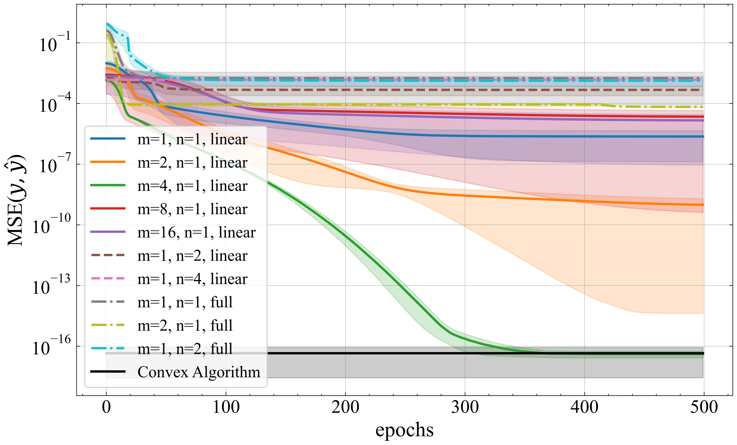
Two synthetic studies examine implications of the theory for practical optimizers: whether more heads aid fitting, and whether the certificate predicts recovery of the ground-truth function. A separate appendix experiment studies finite-automaton execution with a conventional Transformer.
Data come from a random single-head linear-attention teacher on Gaussian sequences of length up to 100. The PDF specifies covariance scaling I/√d for teacher parameters and I/√T for inputs. Models include multi-head single-layer attention, deeper single-head attention, and a full Transformer with softmax, feedforward blocks, and layer normalization.
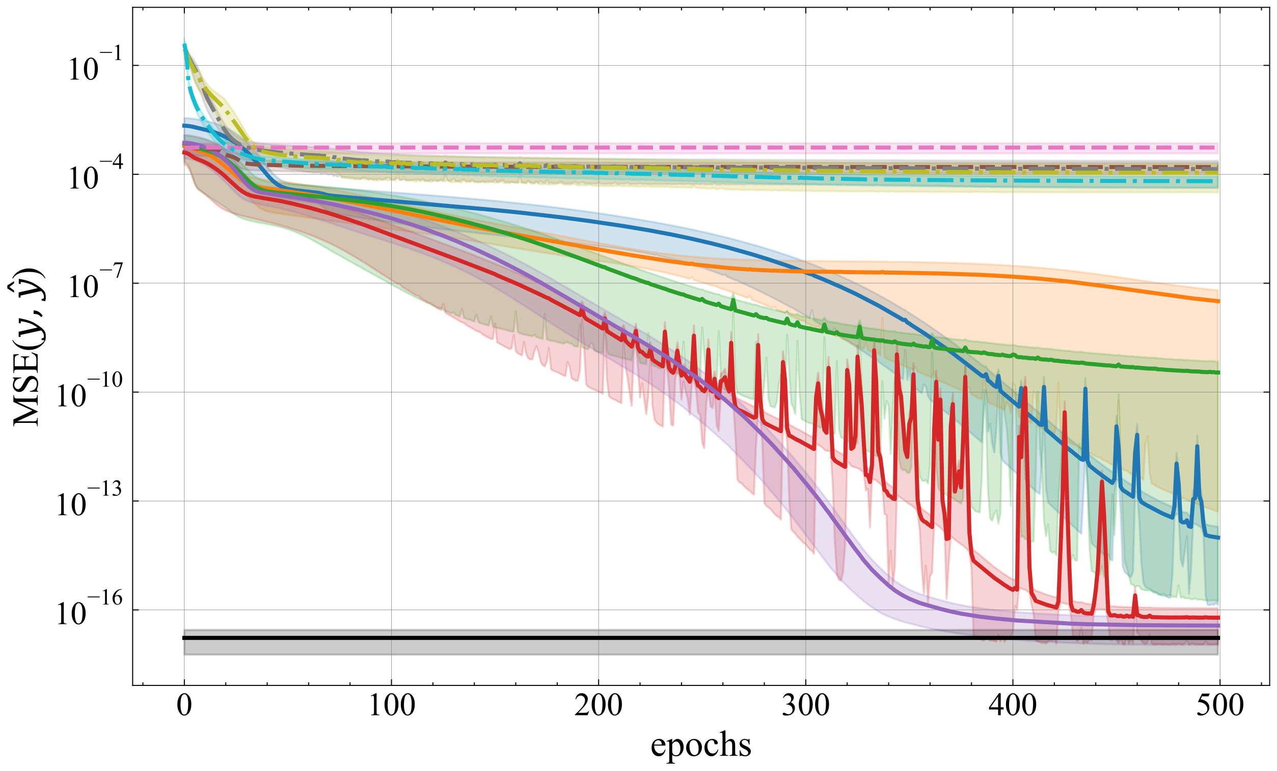
For d = 2 with 512 examples and d = 4 with 2,048 examples, sufficient heads approach the convex method’s numerical error floor. Adding layers or full-Transformer components gives no consistent gain on this deliberately linear-attention-generated task. Shading shows standard error over three runs. These small synthetic experiments support an optimization pattern, not a general ranking of depth and width on language tasks.
Equations
(a)
(b)
Figure 1: Performance comparison of multi-head, multi-layer linear attention models and the original Transformer model (denoted as full). We trained using SGD on synthetic data generated from a single-layer linear attention model for varying training set sizes () and input dimensions (), number of heads , and number of layers . Results demonstrate that multi-head architectures converge faster on different input dimensions and match the performance of our algorithm 1 (convex algorithm). Increasing the number of layers or incorporating multilayer perceptrons (MLPs) and layer normalization did not yield consistent improvements. Shading indicates the standard error over three different runs.
4.2 Does certifiable identifiability predict generalization?
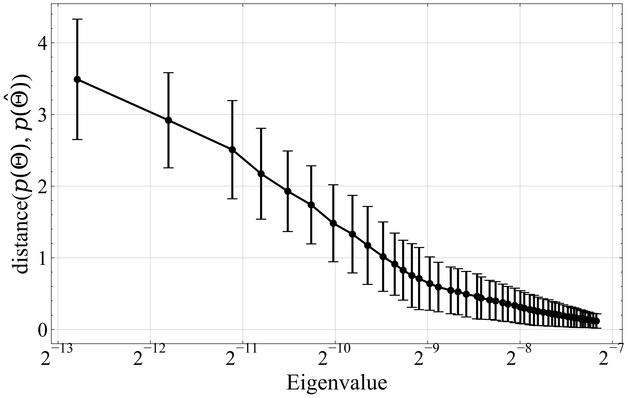
The associative-memory experiment varies the feature-moment eigenvalue and measures distance to the teacher in coefficient space. This connects the certificate to functional recovery rather than ordinary parameter matching.
(a)Certificate of identifiability in form of the minimum Eigenvalue vs. Euclidean distance in feature space of parameters learned by Algorithm 1.
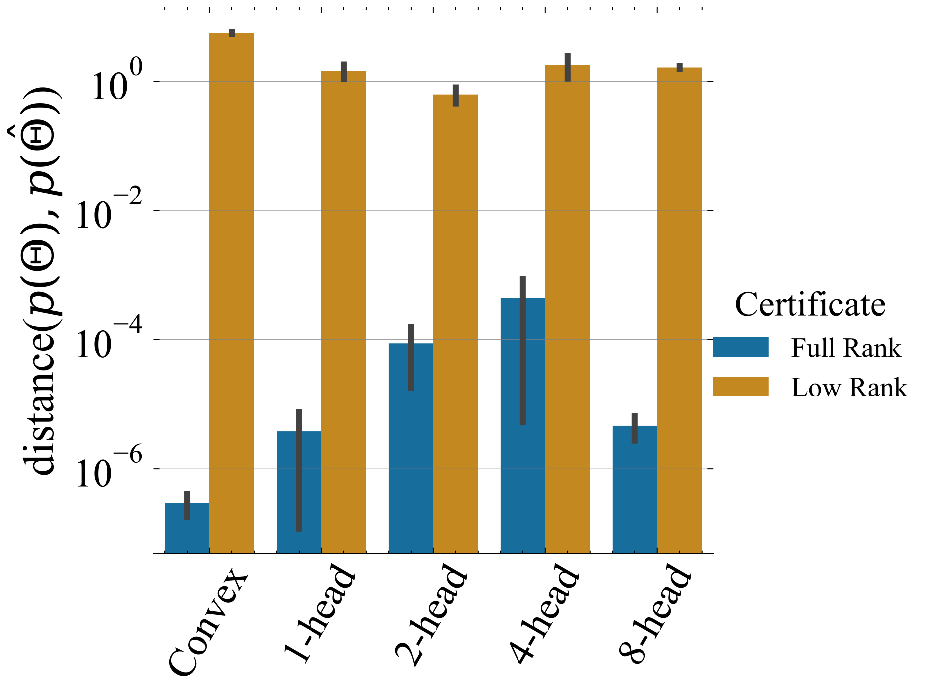
(b)Distance to ground truth parameters in feature space for certifiably identifiable data (min eigenvalue ) vs. nonidentifiable data (min eigenvalue ). Here the parameters of MHLA are learned via SGD. Error bars are standard error on three different runs.
Figure 2: Impact of data distribution on the associative lookup task performance: We generated training data for an associative lookup task (Bietti et al., 2023; Cabannes et al., 2024) using mixtures of two distributions: (1) Gaussian key and value vectors, and (2) random unitary key and value vectors. By adjusting the mixture probability, we can manipulate the certificate value (minimum eigenvalue of the data covariance matrix), as unitary key–value vectors give rank-deficient “certificates”. (a) Algorithm 1: as the minimum eigenvalue increases, Algorithm 1 converges more closely to the true parameters. (b) SGD: SGD learns parameters that are equivalent to the ground truth parameters in feature space for certifiably identifiable data, but for unidentifiable data, they are far apart in feature space and therefore compute different functions.
Associative Memory
The task, following Bietti et al. and Cabannes et al., returns a weighted sum of stored values, with weights given by query–key inner products. The retained block matrices define a single-head teacher. Orthogonal keys reduce this weighted retrieval to an exact lookup; Gaussian keys generally produce a mixture.
Equations 14–15
(14)
(15)
Mixture of distributions:
Keys and values are either Gaussian or columns of independently drawn orthogonal matrices; the query is a uniformly chosen stored key. With d = 4 and 2¹⁴ examples per source dataset, mixtures containing 95–100% orthogonal examples produce progressively weaker certificates. The paper reports full-rank Gaussian data and rank-deficient orthogonal data in this experiment.
Certifiable Identifiability for Algorithm 1 :
After Algorithm 1 fits each mixture, the authors compare its coefficient representation p with the teacher’s. Figure 2a shows smaller coefficient error as the minimum eigenvalue increases. The statistic measures how well the function is identified; it is not directly a held-out task-success rate.
For gradient-trained models with one, two, four, or eight heads, the full-rank dataset has certificate value 0.06 and the deficient dataset has value zero. Learned coefficients are close to the teacher in the former and substantially different in the latter. The theorem applies to an optimizer only insofar as it actually attains the required empirical risk.
5 Related Work
Related work separates representational expressivity, sample requirements, and the computational difficulty of fitting attention.
5.1 Formal Expressivity of Transformers
Earlier work implements circuits, logical expressions, domain-specific languages, formal-language recognizers, and Turing machines with attention. These expressivity results, including Turing completeness, do not themselves supply an efficient learner or a check that a given dataset uniquely identifies the intended computation.
5.2 Learning Transformers
Statistical bounds need not give tractable training algorithms. Earlier optimization results often fix attention parameters, assume structured data, or require favorable initialization and separability. The comparisons include multi-head overparameterization and learning under Bernoulli/Gaussian input assumptions. The present regression lifting targets a simpler unnormalized single-layer class with variable width.
6 Conclusion and Limitations
The main contribution is a concrete way to turn sufficient attention width into convex empirical optimization, together with a data-dependent certificate for functional identification. The model excludes softmax, learned nonlinear intermediate representations, and the multiple interacting layers of modern language models.
The paper proposes extensions through key-query feature maps. Their practicality depends on the size and computability of the resulting representation; the present proof should not be read as an efficient training guarantee for arbitrary learned kernels or full Transformers. Source statements and proofs are retained below, including the qualifications noted for their quantitative bounds.
Acknowledgments
The authors acknowledge NSF, AFOSR, ONR, ARO, Open Philanthropy, MIT Quest for Intelligence, the MIT–IBM Watson AI Lab, the Simons Center for the Social Brain, and an Alexander von Humboldt professorship.
Appendix A Certificate for identifiability of linear attention
Identifiability means that every empirical minimizer computes the same function on all inputs. Realizability means that some model exactly produces the observed labels. Algorithm 2 constructs distinct pair and square features; a full-rank empirical second moment makes the corresponding least-squares coefficient vector unique.
The formal results below distinguish realizable fixed-width models, sufficiently wide models with arbitrary labels, population input-noise claims, and approximate minimizers. The compact coefficient formula in Corollary A.4 should be read with Appendix E’s separate diagonal formula; doubling a diagonal term would give the wrong expansion.
The error statements are preserved as printed. Lemma A.7 defines its set using absolute squared training error, not excess error above a nonzero optimum. Its displayed conclusion uses an unsquared output norm, while the proof bounds a squared norm and omits constants when comparing two approximate fits. It supports a conditioning-dependent stability interpretation, not direct reuse of the printed bound without checking these details.
Algorithm 2 Constructing Features for Certificates of Identifiability
1:Input: Data for
2:Output: feature vectors for
3:fordo
4: Let be the rows of and let be the entry of
5:fordo
6:fordo
7:
8:endfor
9:endfor
10:fordo
11:fordo
12:
13:endfor
14:endfor
15:endfor
16:Return:
Definition A.1 (Identifiability) .
Let . Let denote a model class which is a uniform circuit family parameterized by parameters . Let be a loss function and be the set of empirical risk minimizers:
We say model class is identifiable with respect to the dataset if for all , and for all pairs of empirical risk minimizers we have and compute the same function, i.e., they agree on all inputs (are the same uniform circuit family):
Equations 17–18
(17)
(18)
Definition A.2 (Realizability) .
Let be an MHLA parameterization. We say a dataset is realizable by a parameterization if .
Lemma A.3 (Certificate of Identifiability) .
Let dataset be a realizable dataset. Let be a family of polynomials for defined as follows. We index the entries of by taking the Kronecker product between all sets of pairs (for all ) with with all . We define as in Algorithm 2 to be
Then if , we have that is identifiable with respect to .
Equation 19
(19)
Corollary A.4 .
Let be a collection of polynomials such that
is defined as follows. Each is indexed by pairs for and defined to be
Let the polynomial be . Then for any pair of parameters we have if and only if .
Let be a realizable dataset. Let be drawn from a distribution where the -th entry of denoted by is drawn i.i.d. from a distribution over for all and . Let the second and fourth moment of be denoted and respectively. Let and . Then for is identifiable with respect to . That is to say, for any population risk minimizers :
Equation 21
(21)
Lemma A.6 (Identifiability without realizability for MHLA with arbitrarily many heads) .
Let dataset be any dataset drawn i.i.d from a distribution . Let be defined as in Lemma A.3. Then if then for for any is identifiable with respect to the data . That is,
for all pairs of empirical risk minimizers .
Equation 22
(22)
Lemma A.7 (Identifiability with Error) .
Let be the set of -approximate empirical risk minimizers,
Then we have for any that for all inputs
Equations 23–24
(23)
(24)
Application to learning Universal Turing Machines.
Combining the bounded simulator construction with the certificate yields agreement throughout the stated finite-size domain. The inverse certificate margin enters the runtime through the fitting precision needed for reliable token rounding.
Lemma A.8 (Learning UTM from Certifiably Identifiable Data) .
Let be a dataset satisfying for being the expressibility parameters of Lemma B.1 for the set of TM’s/words . If is certifiably identifiable with , then there is a time algorithm that outputs a set of parameters such that for all TM’s and input words in , we have
The step of the autoregressive computation history of is equal to the ’th step of the computation history of on .
Equation 25
(25)
Appendix B Realizability of Universal Automata in MHLA
The expressivity construction encodes symbols, states, and positions with orthogonal vectors. Lookup, copy, and conditional update primitives append each successive computation-history symbol. It uses O(n̂Φ̂Σ̂) heads and embedding dimension O(n̂Φ̂Σ̂·max(Σ̂,Q̂)), with two-bit construction precision and O((n+t)t) autoregressive steps to represent t machine steps.
These resource bounds grow with the prescribed input/history limits. The construction is a bounded simulator, not a fixed finite-dimensional machine executing arbitrarily long histories without changing its encoding budget.
Let be the set of Turing machines and words with number of states, size of alphabet, size of input, and number of steps in computation history bounded by respectively.
For any , let be the computation history of the UTM on . Let the autoregressive computation history (see Definition C.2) of on input be denoted . Then there exists a set of parameters for and embedding dimension , such that for all , the TM computation history at time step is equivalent to the autoregressive computation history at time step where i.e . Furthermore, this can be achieved with 2 bits of precision.
Appendix C Application to Learning Universal Turing Machines
Autoregressive attention appends each predicted token to its context. Computation histories record that growing sequence, and a decoding convention identifies the suffix representing a simulated tape. The definitions below make the machine description, word, state space, and runtime restriction explicit.
Training examples are intermediate histories paired with their next tokens. Lemma C.5 first invokes the regression generalization result, then rounds predictions and uses a union bound to control failure over the simulated history. This separates on-distribution trace accuracy from the stronger, certificate-dependent out-of-distribution claim. The number of independent machine/word draws must be distinguished from the dependent tokens within each trace.
Let be a TM. Let be all strings in the alphabet . Then let be the language .
Definition C.4 .
(Polynomially Bounded Universal Turing Machine) In general, a UTM is a recognizer for the language . That is if is in , the UTM accepts, else, the UTM rejects or does not halt. Let
be the language of input pairs for TM and word such that decides in polynomial time. Here, we consider UTM to be the polynomial time decider for .
Let in dimension be the MHLA parameters in Lemma B.1. Let be pairs of TM’s and words of maximum length drawn i.i.d. from a distribution . Let . For each TM/word pair let be the -step autoregressive computation history of on . Let be the dataset where . Then Algorithm 1 applied to input returns for such that with probability
for sample complexity . Then with probability over the randomness in the data, the probability over that the -step autoregressive computation history and differ is upper bounded by
Equations 28–29
(28)
(29)
Appendix D Proof of the Main Theorem
Expanding the squared loss shows that each prediction is linear in the lifted parameter matrix. Least squares finds its optimum, and SVD recovers an equivalent attention layer with at most d² heads. Thus the constructive argument concerns fitting the best representable lifted predictor, regardless of whether labels are realizable.
The proof’s final inequality prints absolute training loss ≤ ε, although the preceding agnostic argument bounds loss relative to the optimum. With irreducible label error, that absolute claim does not follow. The original equation is preserved; the useful conclusion is comparison with the best fit. The population-rate step invokes classical learning theory without spelling out squared-loss boundedness or tail conditions.
Equations 30–35
(30)
(31)
(32)
(33)
(34)
(35)
Appendix E Proofs from Identifiability Section
The general certificate writes a model as an inner product between parameter polynomials and input features. In the realizable case, every empirical minimizer reaches zero loss; a positive-definite feature second moment gives a unique coefficient vector. Hence all minimizers agree everywhere, despite possible parameter redundancy.
For linear attention, group the symmetric off-diagonal products and handle row-square terms separately. Equations in this section give both coefficient formulas and reconstruct the output exactly. At width at least d², SVD makes the coefficient map surjective, so uniqueness of least squares no longer needs realizability.
The independent-input proof centers and normalizes features, then analyzes pair–pair, square–square, and mixed moments. Its printed moment calculations have additional subtleties: for example, overlapping indices can involve sixth moments, whereas the stated assumptions mention only second and fourth moments. The edition retains the claims and calculations rather than silently strengthening them.
Equations 38–49
(38)
(39)
(40)
(41)
(42)
(43)
(44)
(45)
(46)
(47)
(48)
(49)
Lemma E.1 (General Certificate of Identifiability) .
Let dataset be a dataset realizable by . Let be a collection of polynomials mapping the parameters to a feature space of fixed dimension . Let be a uniform family of polynomials such that . Let and satisfy
for all for all .
Then if , we have
for all empirical risk minimizers . That is, all empirical risk minimizers compute the same function.
Equations 36–37
(36)
(37)
Case 1: Pairs to Pairs, j ≠ k and j ′ ≠ k ′
The pair–pair case claims vanishing cross terms for distinct unordered row pairs and a positive diagonal proportional to m₂³. The displayed calculations express the intended block-diagonal argument; their independence and index-overlap conditions require care.
Equations 50–51
(50)
(51)
Case 2: Singles to Singles, j = k and j ′ = k ′
The square–square case centers row norms by nm₂. The proposed diagonal factor is (m₄ − m₂²)m₂, positive under the lemma’s stated moment inequality, while different rows are treated as uncorrelated.
Equations 52–53
(52)
(53)
Case 3: Singles to Pairs, j = k and j ′ ≠ k ′
The mixed case completes the proposed block decomposition. The stability proof then bounds output differences using coefficient differences, the minimum feature-moment eigenvalue, and a degree-six input-norm factor.
For two models whose squared training errors are each at most ε, their squared disagreement can generally be bounded by 4ε through the triangle inequality, rather than the proof’s unexplained ε. Lemma E.2 adds bounded label noise and bounded training inputs but supplies only a short proof sketch; its constants, concentration assumptions, and norm convention need verification before numerical use.
Equations 54–58
(54)
(55)
(56)
(57)
(58)
Lemma E.2 (Identifiability with Error and Noise in Realizability) .
Let be a dataset such that for i.i.d and bounded.
Let be the set of -approximate empirical risk minimizers.
Let . Then we have for any that for all inputs
Equations 59–60
(59)
(60)
Appendix F Programs Expressible as Fixed Depth Linear Transformer
Tokens represent objects with several finite-valued attributes. Each head performs a linear transformation of a query attribute, looks up a matching key, and maps the retrieved value into an output attribute. Orthogonal encodings implement arbitrary finite lookup maps as matrices.
Algorithm 3 gives the generic program form. Multiple matching keys would sum values, so the simulator’s layout avoids unwanted collisions. Several heads update different attributes in parallel; additional generated tokens provide sequential operations.
The embedding stores the transition table separately from the word, positional codes, and current state. Disjoint coordinate blocks distinguish intermediate stages; shared coordinates are used deliberately for lookup tables. Each simulated tape symbol consumes a small block of generated tokens.
Algorithms 6–7 combine neighboring tape cells with a transition-table lookup, then handle locations left of, at, and right of the head. The original pseudocode is retained, including Algorithm 7’s repeated “move == L” conditions at lines 13 and 17; it should be checked as a construction sketch before implementation.
Definition F.2 (Embedding) .
Let be a TM over state space , alphabet , transition function . Then
Let be "positional encodings" that assign unique id’s for every letter in the word .
Then we define Embedding(M,x) to be
Equations 61–63
(61)
(62)
(63)
Lookup:
Lookup uses identity query/value transformations to retrieve the value associated with the current token’s selected attribute and write it into the next token.
Copy:
Copy is a lookup by positional code. A fixed permutation shifts the query to an earlier position, allowing an attribute at a prescribed offset to be copied forward.
If-Then:
Conditional updates are compiled into a temporary table: successive dummy tokens store candidate condition/value pairs, then a lookup selects the matching output. Algorithms 4–5 retain the ordinary and attention-program versions; Algorithms 6–7 retain the simulator’s full instruction and branch listings.
Algorithm 4 If-Then Program
1: # If attribute x is equal to any of then set attribute to respectively
The in-distribution argument converts per-step prediction error to a probability of an incorrect rounded token, then unions over a bounded trace. Increasing the sample budget to reduce each step’s error yields the stated history-level guarantee.
For certified data, the smallest eigenvalue bounds coefficient disagreement on every input within the prescribed size budget. Fitting to sufficiently small error then permits consistent token decoding across that budget. These conclusions inherit the quantitative stability and generalization qualifications discussed above; the certificate does not itself supply representative traces.
Equations 65–69
(65)
(66)
(67)
(68)
(69)
Corollary F.3 .
In particular, for sample complexity , by Lemma B.1, we have with probability over the randomness in the data that the probability that the step of the computation history of is equal to is
where . That is, the computation history of the MHLA returned by algorithm 1 is equal to the computation history of on .
Equation 64
(64)
Appendix G Additional Definitions
Orthogonal token embeddings and nearest-token rounding define the symbolic interpretation of vector predictions. Algorithm 8 retains the complete cubic-feature extraction routine used by the regression algorithm.
Algorithm 8 Extract Features
1:Input: Data for and
2:fordo
3: Let be the rows of and let be the entry of
4:fordo
5:fordo
6:fordo
7: Let be defined as follows
8:
9:endfor
10:endfor
11:endfor
12:endfor
13:Return: such that Equation 70
(70)
Definition G.1 (Orthogonal Embeddings) .
Let Embed be a function . Let be an alphabet and let be a basis of orthogonal unit vectors. Then for each letter in an alphabet , we define where we associate a different unit vector to each letter.
Definition G.2 (Rounding) .
For any vector , let for . Since we use orthogonal unit vectors for token embeddings we will refer to as a token. We will often refer to a matrix as being equivalent to a series of tokens to mean for all .
G.1 Training details of attention networks
The retained search table varies input dimension 2–16, heads 1–16, depth 1–4, learning rate 0.01/0.001, and batch size 32/64. The prose names Adam while the table specifies AdamW. This distinction is preserved instead of treating the experimental optimizer as uniquely specified.
The finite-automaton experiment uses a Llama-style Transformer with four layers, sixteen heads, hidden dimension 2,048, learning rate 0.00025, and 100 epochs. Training-set sizes range from 16 to 65,536 examples, with intermediate settings listed in the source; the complete hyperparameter table is retained.
Figure 3 repeats the d = 4, N = 2,048 synthetic attention comparison, showing the error curves against training epoch. Its three-run uncertainty and the convex solver’s numerical floor should be kept in view when comparing convergence.
(a)Figure 3: Performance comparison of multi-head, multi-layer linear attention models and the original Transformer model (denoted as full). We trained using SGD on synthetic data generated from a single-layer linear attention model for varying training set sizes () and input dimensions (), number of heads , and number of layers . We present mean squared error of the predictions w.r.t number of training epochs. Results demonstrate that multi-head architectures converge faster on different input dimensions and match the performance of our algorithm 1 (convex algorithm). Increasing the number of layers or incorporating multilayer perceptrons (MLPs) and layer normalization did not yield consistent improvements. Shading indicates the standard error over three different runs.
G.4 Learning the Computation History of Deterministic Finite Automata
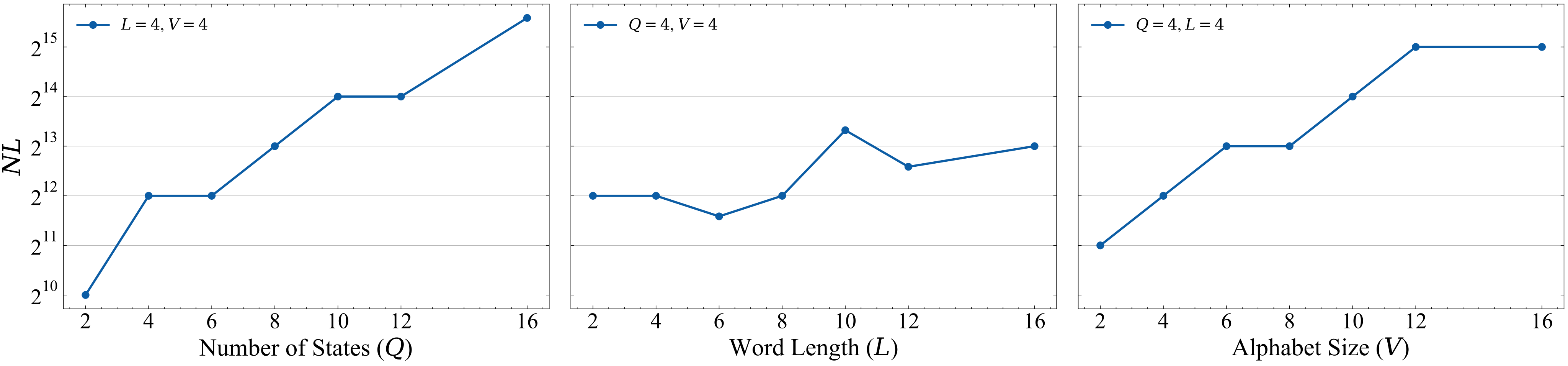
The task supplies an explicit finite-automaton transition table and input word, and asks for the visited-state history. It tests executing a described automaton, rather than inferring an unknown transition system solely from examples. Although the introduction to this experiment mentions MHLA, its reported model is the conventional four-layer Transformer described in Section G.2.
Figure 4: Data requirement for universal DFA simulation: We train a fixed sized Transformer (4-layers, 16 heads and 2048 hidden dimensions) to simulate a DFA given a transition table and input word. The vertical axis shows the number of tokens (expressed as word length times the number of examples ) required to obtain 99% next token accuracy.
Dataset
Each transition is encoded by a parenthesized state–symbol–next-state triplet. The model receives all transitions and the word, then predicts the history autoregressively with cross-entropy loss. The transition-table description uses five tokens per state/symbol pair, including parentheses.
Equation
Results
Figure 4 varies states, word length, or alphabet size while fixing the other two at four. It reports the smallest training-token budget reaching 99% next-token accuracy. The curves are suggestive of subexponential scaling over the tested range; they neither prove polynomial scaling nor establish 99% accuracy for complete histories.
47 references
Ahn et al. [2024]
Kwangjun Ahn, Xiang Cheng, Minhak Song, Chulhee Yun, Ali Jadbabaie, and Suvrit Sra.
Linear attention is (maybe) all you need (to understand transformer optimization), 2024.
URLhttps://arxiv.org/abs/2310.01082.
Akyürek et al. [2024]
Ekin Akyürek, Bailin Wang, Yoon Kim, and Jacob Andreas.
In-context language learning: Architectures and algorithms, 2024.
URLhttps://arxiv.org/abs/2401.12973.
Barceló et al. [2020]
Pablo Barceló, Egor V Kostylev, Mikael Monet, Jorge Pérez, Juan Reutter, and Juan-Pablo Silva.
The logical expressiveness of graph neural networks.
In ICLR, 2020.
Barceló et al. [2024]
Pablo Barceló, Alexander Kozachinskiy, Anthony Widjaja Lin, and Vladimir Podolskii.
Logical languages accepted by transformer encoders with hard attention.
2024.
Beck et al. [2024]
Maximilian Beck, Korbinian Pöppel, Markus Spanring, Andreas Auer, Oleksandra Prudnikova, Michael Kopp, Günter Klambauer, Johannes Brandstetter, and Sepp Hochreiter.
xLSTM: Extended long short-term memory.
Vancouver, Canada, December 2024.
Bietti et al. [2023]
Alberto Bietti, Vivien Cabannes, Diane Bouchacourt, Herve Jegou, and Leon Bottou.
Birth of a transformer: A memory viewpoint, 2023.
URLhttps://arxiv.org/abs/2306.00802.
Cabannes et al. [2024]
Vivien Cabannes, Berfin Simsek, and Alberto Bietti.
Learning associative memories with gradient descent, 2024.
URLhttps://arxiv.org/abs/2402.18724.
Chiang et al. [2023]
David Chiang, Peter Cholak, and Anand Pillay.
Tighter bounds on the expressivity of transformer encoders.
arXiv preprint arXiv:2301.10743, 2023.
Dao and Gu [2024]
Tri Dao and Albert Gu.
Transformers are ssms: Generalized models and efficient algorithms through structured state space duality, 2024.
URLhttps://arxiv.org/abs/2405.21060.
Deora et al. [2023]
Puneesh Deora, Rouzbeh Ghaderi, Hossein Taheri, and Christos Thrampoulidis.
On the optimization and generalization of multi-head attention, 2023.
URLhttps://arxiv.org/abs/2310.12680.
Edelman et al. [2022a]
Benjamin L. Edelman, Surbhi Goel, Sham Kakade, and Cyril Zhang.
Inductive biases and variable creation in self-attention mechanisms, 2022a.
URLhttps://arxiv.org/abs/2110.10090.
Edelman et al. [2022b]
Benjamin L Edelman, Surbhi Goel, Sham Kakade, and Cyril Zhang.
Inductive biases and variable creation in self-attention mechanisms.
In International Conference on Machine Learning, pages 5793–5831. PMLR, 2022b.
Feng et al. [2023]
Guhao Feng, Yuntian Gu, Bohang Zhang, Haotian Ye, Di He, and Liwei Wang.
Towards revealing the mystery behind chain of thought: a theoretical perspective.
arXiv preprint arXiv:2305.15408, 2023.
Fu et al. [2023]
Hengyu Fu, Tianyu Guo, Yu Bai, and Song Mei.
What can a single attention layer learn? a study through the random features lens, 2023.
URLhttps://arxiv.org/abs/2307.11353.
Hahn [2020]
Michael Hahn.
Theoretical limitations of self-attention in neural sequence models.
Transactions of the Association for Computational Linguistics, 8:156–171, 2020.
Hao et al. [2022]
Yiding Hao, Dana Angluin, and Robert Frank.
Formal language recognition by hard attention transformers: Perspectives from circuit complexity.
Transactions of the Association for Computational Linguistics, 10:800–810, 2022.
Jelassi et al. [2022]
Samy Jelassi, Michael E. Sander, and Yuanzhi Li.
Vision transformers provably learn spatial structure, 2022.
URLhttps://arxiv.org/abs/2210.09221.
Katharopoulos et al. [2020]
Angelos Katharopoulos, Apoorv Vyas, Nikolaos Pappas, and François Fleuret.
Transformers are rnns: Fast autoregressive transformers with linear attention, 2020.
URLhttps://arxiv.org/abs/2006.16236.
Kearns and Vazirani [1994]
Michael J. Kearns and Umesh Vazirani.
An Introduction to Computational Learning Theory.
The MIT Press, 08 1994.
ISBN 9780262276863.
doi: 10.7551/mitpress/3897.001.0001.
URLhttps://doi.org/10.7551/mitpress/3897.001.0001.
Li et al. [2024]
Zhiyuan Li, Hong Liu, Denny Zhou, and Tengyu Ma.
Chain of thought empowers transformers to solve inherently serial problems.
arXiv preprint arXiv:2402.12875, 2024.
Liu et al. [2022]
Bingbin Liu, Jordan T Ash, Surbhi Goel, Akshay Krishnamurthy, and Cyril Zhang.
Transformers learn shortcuts to automata.
arXiv preprint arXiv:2210.10749, 2022.
Merrill and Sabharwal [2023]
William Merrill and Ashish Sabharwal.
The parallelism tradeoff: Limitations of log-precision transformers.
Transactions of the Association for Computational Linguistics, 11:531–545, 2023.
Merrill et al. [2021]
William Merrill, Yoav Goldberg, and Noah A Smith.
On the power of saturated transformers: A view from circuit complexity.
arXiv preprint arXiv:2106.16213, 2021.
Merrill et al. [2022]
William Merrill, Ashish Sabharwal, and Noah A Smith.
Saturated transformers are constant-depth threshold circuits.
Transactions of the Association for Computational Linguistics, 10:843–856, 2022.
Oymak et al. [2023]
Samet Oymak, Ankit Singh Rawat, Mahdi Soltanolkotabi, and Christos Thrampoulidis.
On the role of attention in prompt-tuning, 2023.
URLhttps://arxiv.org/abs/2306.03435.
Pérez et al. [2019]
Jorge Pérez, Javier Marinković, and Pablo Barceló.
On the turing completeness of modern neural network architectures.
In ICLR, 2019.
Pérez et al. [2021]
Jorge Pérez, Pablo Barceló, and Javier Marinkovic.
Attention is turing complete.
The Journal of Machine Learning Research, 22(1):3463–3497, 2021.
Schlag et al. [2021]
Imanol Schlag, Kazuki Irie, and Jürgen Schmidhuber.
Linear Transformers are secretly fast weight programmers.
Virtual only, July 2021.
Strobl et al. [2024]
Lena Strobl, William Merrill, Gail Weiss, David Chiang, and Dana Angluin.
What formal languages can transformers express? a survey.
Transactions of the Association for Computational Linguistics, 12:543–561, 2024.
Sun et al. [2023]
Yutao Sun, Li Dong, Shaohan Huang, Shuming Ma, Yuqing Xia, Jilong Xue, Jianyong Wang, and Furu Wei.
Retentive network: A successor to transformer for large language models.
Preprint arXiv:2307.08621, 2023.
Tian et al. [2023]
Yuandong Tian, Yiping Wang, Beidi Chen, and Simon Du.
Scan and snap: Understanding training dynamics and token composition in 1-layer transformer, 2023.
URLhttps://arxiv.org/abs/2305.16380.
Touvron et al. [2023]
Hugo Touvron, Louis Martin, Kevin Stone, Peter Albert, Amjad Almahairi, Yasmine Babaei, Nikolay Bashlykov, Soumya Batra, Prajjwal Bhargava, Shruti Bhosale, et al.
Llama 2: Open foundation and fine-tuned chat models.
arXiv preprint arXiv:2307.09288, 2023.
Trauger and Tewari [2023]
Jacob Trauger and Ambuj Tewari.
Sequence length independent norm-based generalization bounds for transformers, 2023.
URLhttps://arxiv.org/abs/2310.13088.
Vaswani et al. [2017]
Ashish Vaswani, Noam Shazeer, Niki Parmar, Jakob Uszkoreit, Llion Jones, Aidan N Gomez, Łukasz Kaiser, and Illia Polosukhin.
Attention is all you need.
Advances in neural information processing systems, 30, 2017.
Wei et al. [2021]
Colin Wei, Yining Chen, and Tengyu Ma.
Statistically meaningful approximation: a case study on approximating turing machines with transformers.
CoRR, abs/2107.13163, 2021.
URLhttps://arxiv.org/abs/2107.13163.
Weiss et al. [2021]
Gail Weiss, Yoav Goldberg, and Eran Yahav.
Thinking like transformers.
In International Conference on Machine Learning, pages 11080–11090. PMLR, 2021.
Yang et al. [2024]
Songlin Yang, Bailin Wang, Yikang Shen, Rameswar Panda, and Yoon Kim.
Gated linear attention transformers with hardware-efficient training.
Vienna, Austria, July 2024.
Yang et al. [2025]
Songlin Yang, Bailin Wang, Yu Zhang, Yikang Shen, and Yoon Kim.
Parallelizing linear transformers with the delta rule over sequence length, 2025.
URLhttps://arxiv.org/abs/2406.06484.
Zhang et al. [2023]
Ruiqi Zhang, Spencer Frei, and Peter L. Bartlett.
Trained transformers learn linear models in-context, 2023.
URLhttps://arxiv.org/abs/2306.09927.
Zhang et al. [2024]
Yufeng Zhang, Boyi Liu, Qi Cai, Lingxiao Wang, and Zhaoran Wang.
An analysis of attention via the lens of exchangeability and latent variable models, 2024.
URLhttps://arxiv.org/abs/2212.14852.