MultiNash-PF searches for several locally stable joint trajectories in a constrained multi-agent game. A potential-game formulation turns equilibrium search into one constrained optimization problem. Implicit particle filtering locates promising trajectory groups, clustering provides initial guesses, and a nonlinear solver refines each group. In a two-agent obstacle example, recovering six modes takes 3.36 seconds versus 6.71 seconds for repeated random solver initialization. A small human–robot experiment demonstrates choosing between two precomputed passing modes; the method does not guarantee finding every equilibrium.
I Introduction
When two agents pass each other, yielding on either side may work, but incompatible choices can cause a conflict. A robot therefore benefits from considering several outcomes and identifying the other agent’s preference. The proposed pipeline aims to find multiple useful local equilibria efficiently. Its finite sampled search should be distinguished from complete enumeration of all possible behaviors or from knowing that a human will follow the assumed game model.
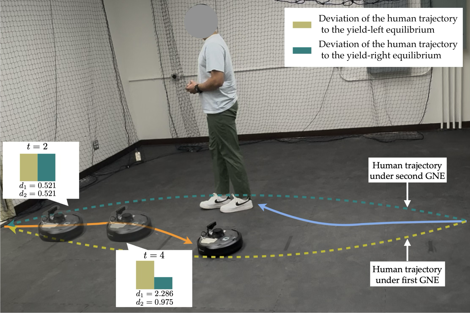
Fig. 1: Snapshot of an interaction between a robot and a human when they exchange positions. Using MultiNash-PF, the robot can compute both modes of interaction. At , the robot is uncertain about the preferred mode of the human since the human trajectory’s distance from both equilibria is almost the same. At , the human trajectory is closer to the yield-right GNE; therefore, the robot chooses the corresponding GNE and avoids collision with the human.
II Related Works
Game-theoretic planners compute interactive trajectories using best responses, local approximations, constrained solvers, or potential games [11]. A single optimization initialization usually returns only one local solution. Repeating random starts can recover more modes but often revisits the same solution. Bayesian trajectory inference and implicit particle filtering [31] motivate a more focused initialization strategy.
III Constrained Potential Trajectory Games
Each agent has continuously differentiable dynamics and a quadratic cost for tracking its reference trajectory and limiting control effort. Individual costs depend only on that agent’s states and controls; shared constraints couple the agents through collision avoidance and other bounds. This restricted cost/constraint structure is what enables the potential-game reduction. It does not represent arbitrary strategic preferences or general-sum games.
Equations 1–3
(1)
(2)
(3)
III-A Local Generalized Nash Equilibrium Trajectories
A local generalized Nash equilibrium is a feasible joint trajectory for which no individual agent can improve its cost by a sufficiently small feasible unilateral change. Because the costs are separable, their sum forms a potential whose local constrained minima are sufficient to produce such equilibria. The retained theorem and proof establish this direction, drawing on the cited potential-game result.
The reverse direction is not guaranteed: finding all local minima of this potential need not find all equilibria of the original game. In addition, the proposed sampled algorithm need not find every potential minimum. The paper acknowledges the first limitation; the demonstrated mode counts are empirical results for specified examples.
Equations 4–6
(4)
(5)
(6)
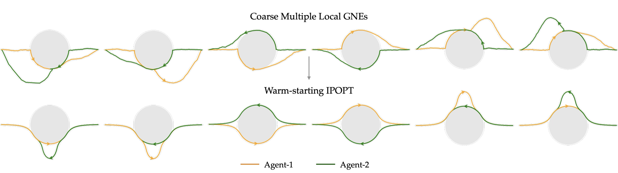
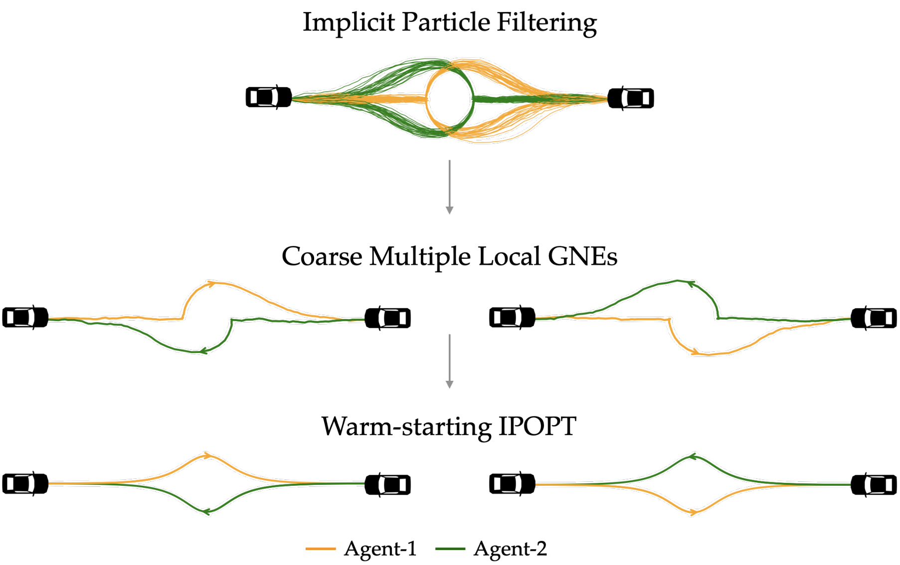
Fig. 2: When using MultiNash-PF on a difficult two agent trajectory game, we first employ an implicit particle filter to obtain coarse estimates of GNEs.
IV Identifying Local Nash Equilibria via Bayesian Inference
The trajectory optimization problem is recast as a virtual state-estimation problem. Reference states act as measurements, and a soft constraint-violation term favors feasible trajectories. Gaussian disturbance models connect high-posterior trajectories to low-cost solutions under the stated assumptions. This inference stage supplies approximate candidates; it does not replace the final constrained solver’s feasibility check.
Each particle describes a complete trajectory. Rather than sample indiscriminately, an implicit map steers samples toward high-probability regions. A bank of unscented Kalman filters supplies local Gaussian approximations to make that map tractable. The approach can reduce particle degeneracy and resampling, but local approximations and finite particles remain sources of missed modes.
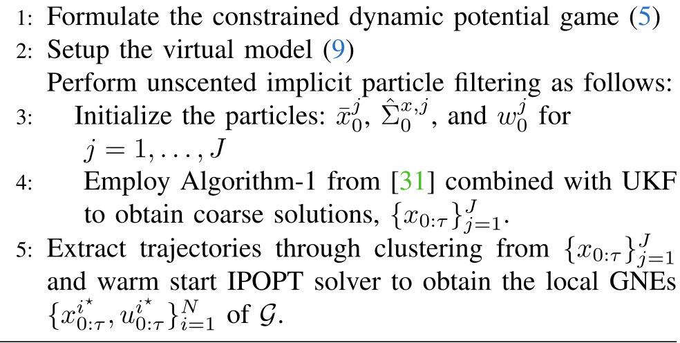
Trajectories are clustered using Fréchet distance, with hierarchical clustering or density-based clustering suggested. Each cluster’s mean initializes IPOPT [24], which refines a constrained local solution. Clustering thresholds and mode coverage affect how many distinct solutions are recovered. Algorithm 1 retains the original PDF’s line grouping and indentation.
Equations 7–10
(7)
(8)
(9)
(10)
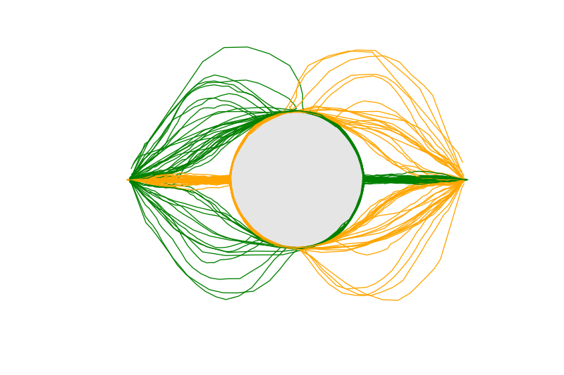
Fig. 3: MultiNash-PF identifies all the local GNE trajectories for a challenging two-agent trajectory game where two agents swapped positions while avoiding an obstacle. In this scenario, the obstacle radius is greater than the collision avoidance radius of the two agents, leading to the discovery of 6 distinct Nash equilibria. MultiNash-PF effectively obtains coarse estimates of local GNEs through implicit particle filtering, which are then refined using IPOPT to obtain local GNEs.Equations 11–12
(11)
(12)
Algorithm 1 MultiNash-PF: Multiple local GNEs based on particle filter
V Numerical Simulations
The simulations use two unicycle agents with position, heading, linear velocity, and angular velocity states. Inputs change the two velocities, and quadratic costs favor straight reference paths. With mutual collision avoidance alone, the experiment recovers left-passing and right-passing equilibria.
A second scenario adds a central obstacle of radius four metres, larger than the three-metre agent separation radius, plus control bounds. Fifty particles recover six reported modes: two pass on opposite sides of the obstacle, and four pass on the same side with different yielding orders. Spatially overlapping curves can still avoid collision because agents traverse them at different times. The evidence is limited to these two-agent scenarios.
Equations 13–14
(13)
(14)
Fig. 4: The Nash equilibrium trajectories found by MultiNash-PF when two unicycle agents change their positions. First, we use the implicit particle filter to discover the coarse estimates of two different equilibria, and then utilize them as a warm start for IPOPT to obtain the two Nash equilibrium trajectories.
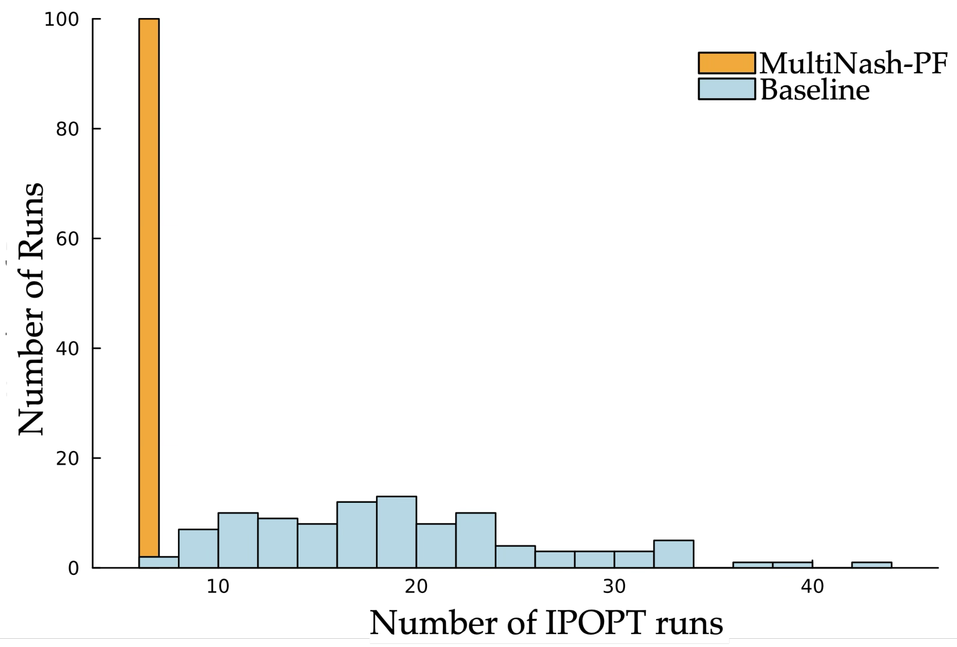
(a)Histogram of the number of IPOPT runs required to obtain all six equilibria.
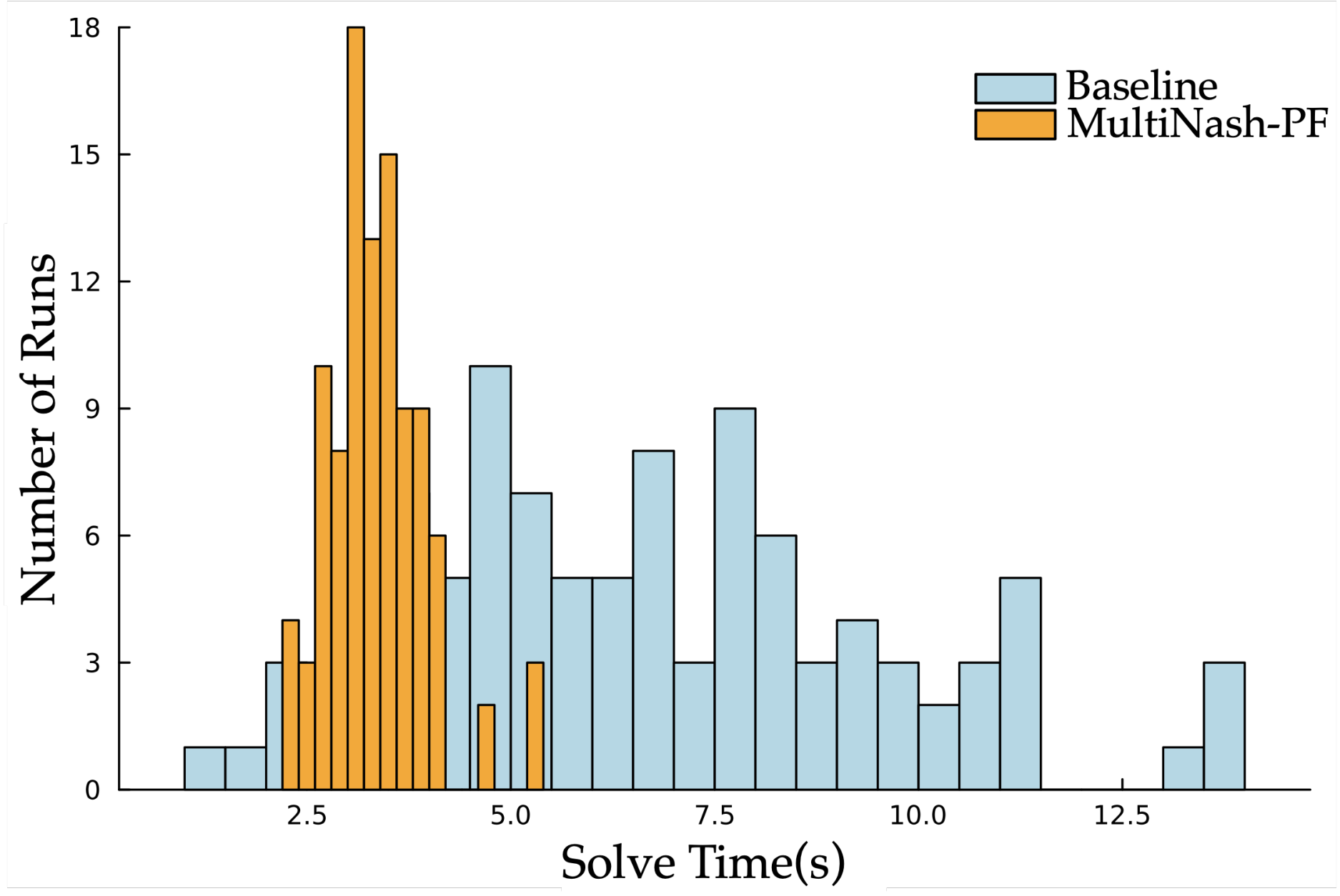
(b)Histogram of the solve time comparison of MultiNash-PF and the baseline.
Fig. 5: Comparison of MultiNash-PF with the baseline for the experiment shown in Fig. 3.
(a) For the baseline, the average number of IPOPT runs required to obtain all six different equilibria is , while for MultiNash-PF, this is always . MultiNash-PF requires 3 times fewer IPOPT runs.
(b) MultiNash-PF reduces the solve time by about compared to the baseline while giving a much lower variance on the solve time.
V- 1 Comparison with Baseline
Over one hundred Monte Carlo runs of the obstacle case, random initialization needs 18.64 ± 7.57 IPOPT solves to recover the six known modes, while the proposed method uses six refinement solves. Total measured time falls from 6.71 ± 2.83 seconds to 3.36 ± 0.59 seconds, approximately a 50% reduction. Filtering accounts for 0.37 ± 0.072 seconds and refinement for 2.99 ± 0.57 seconds. This comparison stops when six previously identified modes have been recovered; it is not a proof of exhaustive equilibrium discovery or a general scaling study.
VI Hardware Experiment
A TurtleBot 4 and one human exchange positions, with both modeled using unicycle dynamics and tracked by Vicon motion capture. The robot precomputes two passing equilibria, then replans with a five-second horizon and 0.1-second discretization during a ten-second interaction. It compares the observed human trajectory with the two candidate human paths using Fréchet distance and selects a mode once their distance difference exceeds a threshold.
In ten trials with the human instructed to choose left or right randomly, the robot identifies the mode, avoids collision, and reaches its goal. This supports the two-mode demonstration but supplies no broad human-subject evaluation, uncertainty calibration, or safety guarantee. The several-second multi-equilibrium search is performed in advance; these trials do not establish real-time recomputation of all modes at every control step.
VII Conclusion
The contribution is a practical initialization pipeline for discovering multiple local interaction modes before constrained refinement. Its strengths are lower repeated-solver cost in the tested example and a physical demonstration of mode adaptation. Coverage depends on sampling and clustering, the equilibrium reduction requires the specified game structure, and larger populations or more complex human behavior are not evaluated.
39 references
[1]
R. Alterman and A. Garland, “Convention in joint activity,” Cognitive Science, vol. 25, no. 4, pp. 611–657, 2001.
[2]
L. Peters, D. Fridovich-Keil, C. J. Tomlin, and Z. N. Sunberg, “Inference-based strategy alignment for general-sum differential games,” arXiv preprint arXiv:2002.04354[cs.RO], 2020.
[3]
J. Im, Y. Yu, D. Fridovich-Keil, and U. Topcu, “Coordination in noncooperative multiplayer matrix games via reduced rank correlated equilibria,” arXiv preprint arXiv:2403.10384[cs.GT], 2024.
[5]
G. Galati, S. Primatesta, S. Grammatico, S. Macrì, and A. Rizzo, “Game theoretical trajectory planning enhances social acceptability of robots by humans,” Scientific Reports, vol. 12, no. 1, p. 21976, 2022.
[6]
D. Fridovich-Keil, E. Ratner, L. Peters, A. D. Dragan, and C. J. Tomlin, “Efficient iterative linear-quadratic approximations for nonlinear multi-player general-sum differential games,” in 2020 IEEE International Conference on Robotics and Automation (ICRA), pp. 1475–1481, IEEE, 2020.
[7]
D. Sadigh, S. Sastry, S. A. Seshia, and A. D. Dragan, “Planning for autonomous cars that leverage effects on human actions.,” in Robotics: Science and systems, vol. 2, pp. 1–9, Ann Arbor, MI, USA, 2016.
[8]
M. Bhatt and N. Mehr, “Strategic decision-making in multi-agent domains: A weighted potential dynamic game approach,” arXiv preprint arXiv:2308.05876, 2023.
[9]
A. Dreves and M. Gerdts, “A generalized Nash equilibrium approach for optimal control problems of autonomous cars,” Optimal Control Applications and Methods, vol. 39, no. 1, pp. 326–342, 2018.
[10]
M. Wang, N. Mehr, A. Gaidon, and M. Schwager, “Game-theoretic planning for risk-aware interactive agents,” in 2020 IEEE/RSJ International Conference on Intelligent Robots and Systems (IROS), pp. 6998–7005, IEEE, 2020.
[11]
M. Bhatt, Y. Jia, and N. Mehr, “Efficient constrained multi-agent trajectory optimization using dynamic potential games,” in 2023 IEEE/RSJ International Conference on Intelligent Robots and Systems (IROS), pp. 7303–7310, IEEE, 2023.
[12]
Y. Jia, M. Bhatt, and N. Mehr, “Rapid: Autonomous multi-agent racing using constrained potential dynamic games,” in 2023 European Control Conference (ECC), pp. 1–8, IEEE, 2023.
[13]
S. Zazo, S. V. Macua, M. Sánchez-Fernández, and J. Zazo, “Dynamic potential games with constraints: Fundamentals and applications in communications,” IEEE Transactions on Signal Processing, vol. 64, no. 14, pp. 3806–3821, 2016.
[14]
I. Askari, X. Tu, S. Zeng, and H. Fang, “Model predictive inferential control of neural state-space models for autonomous vehicle motion planning,” arXiv preprint arXiv:2310.08045, 2023.
[16]
A. Liniger and J. Lygeros, “A noncooperative game approach to autonomous racing,” IEEE Transactions on Control Systems Technology, vol. 28, no. 3, pp. 884–897, 2019.
[17]
R. Spica, E. Cristofalo, Z. Wang, E. Montijano, and M. Schwager, “A real-time game theoretic planner for autonomous two-player drone racing,” IEEE Transactions on Robotics, vol. 36, no. 5, pp. 1389–1403, 2020.
[18]
M. Wang, Z. Wang, J. Talbot, J. C. Gerdes, and M. Schwager, “Game theoretic planning for self-driving cars in competitive scenarios.,” in Robotics: Science and Systems, 2019.
[19]
N. Mehr, M. Wang, M. Bhatt, and M. Schwager, “Maximum-entropy multi-agent dynamic games: Forward and inverse solutions,” IEEE transactions on robotics, vol. 39, no. 3, pp. 1801–1815, 2023.
[20]
S. Le Cleac’h, M. Schwager, and Z. Manchester, “Algames: a fast augmented lagrangian solver for constrained dynamic games,” Autonomous Robots, vol. 46, no. 1, pp. 201–215, 2022.
[21]
T. Kavuncu, A. Yaraneri, and N. Mehr, “Potential iLQR: A potential-minimizing controller for planning multi-agent interactive trajectories,” arXiv preprint arXiv:2107.04926, 2021.
[22]
Z. Williams, J. Chen, and N. Mehr, “Distributed potential ilqr: Scalable game-theoretic trajectory planning for multi-agent interactions,” in 2023 IEEE International Conference on Robotics and Automation (ICRA), pp. 01–07, 2023.
[23]
M. Bhatt, Y. Jia, and N. Mehr, “Strategic decision-making in multi-agent domains: A weighted constrained potential dynamic game approach,” IEEE Transactions on Robotics, 2025.
[24]
A. Wächter and L. T. Biegler, “On the implementation of an interior-point filter line-search algorithm for large-scale nonlinear programming,” Mathematical Programming, vol. 106, no. 1, pp. 25–57, 2006.
[26]
I. Askari, A. Vaziri, X. Tu, S. Zeng, and H. Fang, “Model predictive inferential control of neural state-space models for autonomous vehicle motion planning,” IEEE Transactions on Robotics, vol. 41, pp. 3202–3222, 2025.
[27]
I. Askari, S. Zeng, and H. Fang, “Nonlinear model predictive control based on constraint-aware particle filtering/smoothing,” in 2021 American Control Conference (ACC), pp. 3532–3537, IEEE, 2021.
[28]
I. Askari, B. Badnava, T. Woodruff, S. Zeng, and H. Fang, “Sampling-based nonlinear MPC of neural network dynamics with application to autonomous vehicle motion planning,” in 2022 American Control Conference (ACC), pp. 2084–2090, IEEE, 2022.
[31]
I. Askari, M. A. Haile, X. Tu, and H. Fang, “Implicit particle filtering via a bank of nonlinear Kalman filters,” Automatica, vol. 145, p. 110469, 2022.
[32]
I. Askari, A. Vaziri, X. Tu, S. Zeng, and H. Fang, “Model predictive inferential control of neural state-space models for autonomous vehicle motion planning,” IEEE Transactions on Robotics, 2025.
[33]
C. Daskalakis, P. W. Goldberg, and C. H. Papadimitriou, “The complexity of computing a Nash equilibrium,” Communications of the ACM, vol. 52, no. 2, pp. 89–97, 2009.
[35]
E. A. Wan and R. Van Der Merwe, “The unscented kalman filter for nonlinear estimation,” in Proceedings of the IEEE 2000 adaptive systems for signal processing, communications, and control symposium (Cat. No. 00EX373), pp. 153–158, Ieee, 2000.
[36]
F. Murtagh and P. Contreras, “Algorithms for hierarchical clustering: an overview,” Wiley Interdisciplinary Reviews: Data Mining and Knowledge Discovery, vol. 2, no. 1, pp. 86–97, 2012.
[37]
M. Ester, H.-P. Kriegel, J. Sander, X. Xu, et al., “A density-based algorithm for discovering clusters in large spatial databases with noise,” in kdd, vol. 96, pp. 226–231, 1996.