At a glance
This paper separates an agent’s observation model from its motion policy when predicting or imitating navigation. Viewing range, viewing angle, missed detections, and sensor direction affect which obstacles can influence an action. Synthetic experiments estimate these components one at a time; an eight-person game study supplies demonstrations for a diffusion policy that jointly moves and looks. Learned observation control reduces obstacle proximity relative to a fixed-rotation baseline, and a small car demonstrates transfer to a static-obstacle laboratory setting.
I INTRODUCTION
A trajectory that appears irrational under full visibility can be reasonable for someone who has not seen an obstacle. The proposed decomposition models both what an agent can observe and how it acts on those observations. Related imitation methods infer rewards, clone actions, or learn generative policies; here the observation interface is made explicit. Three experiments infer field-of-view parameters, detection probability, or policy while treating the remaining components as known. Consequently, the paper demonstrates conditional estimation rather than joint identification of every hidden perceptual and behavioral variable from unrestricted human motion.
II METHODOLOGY
II-A Problem Formulation
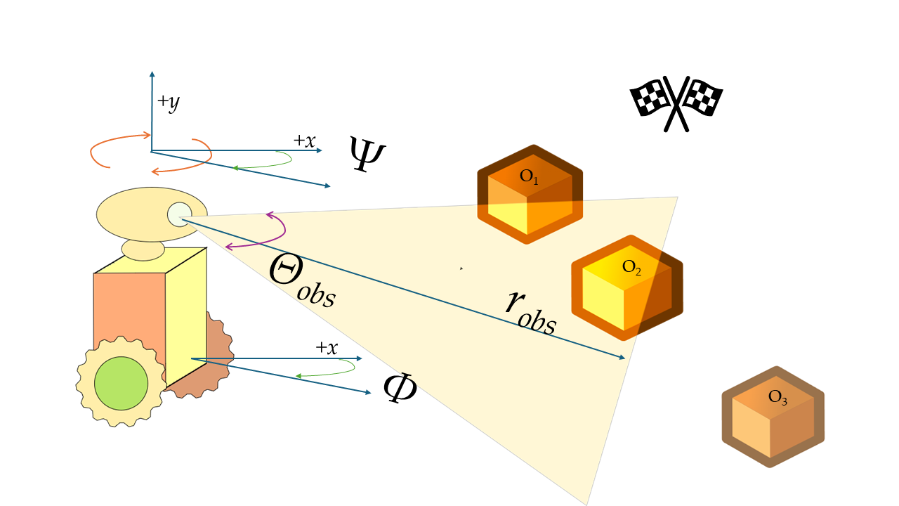
The formulation uses known deterministic state dynamics and a stochastic observation function parameterized by viewing geometry and detection probability. A policy maps an observation to an action. Demonstrations contain states and controls over time. In the running example, the base and visual sensor can turn independently; actions therefore include both movement and sensing direction. Although motivated through a partially observable Markov decision process, the presented policy is observation-conditioned and the paper does not derive a general belief-state inference algorithm. The modular experiments assume sufficient access to environment geometry and demonstrations to evaluate candidate observation models.
Equations 1–3
| (1) |
| (2) |
| (3) |
II-B Estimating the Observation Space
Assumption 1 fixes the policy and probability of detecting an obstacle. Candidate viewing ranges and angles are scored by trajectory likelihood, integrating over possible observations at each step. Equation 5 maximizes a sum of log likelihoods; the cross-entropy method [24] searches the parameter space without differentiating through perception and policy. The preceding prose writes dataset probability as a sum of trajectory probabilities, which is inconsistent with the independent-trajectory product associated with the stated log-likelihood objective. The original equations remain available for inspection; the empirical procedure is best read as the authors’ black-box likelihood search.
Equations 4–5
| (4) |
| (5) |
II-C Estimating the Probability of Observation
Assumption 2 fixes viewing geometry and policy, leaving a single unknown detection probability. Equation 6 applies the analogous likelihood objective, optimized with Bayesian optimization. This estimates a constant detection probability in the synthetic setting; it does not recover object-specific salience, attention history, or a realistic model of human perceptual errors.
Equation 6
| (6) |
II-D Estimating the Policy of the Agent
With viewing geometry known, policy learning becomes behavior cloning on the demonstrator’s restricted observations. A denoising diffusion policy predicts actions conditioned on state and observation. This avoids giving the learner obstacle information unavailable to its demonstrator. The method follows existing diffusion-policy machinery [21] rather than deriving a new denoising objective, and the separately estimated detection parameters are not shown to be jointly identified with the learned policy.
III Numerical Simulations
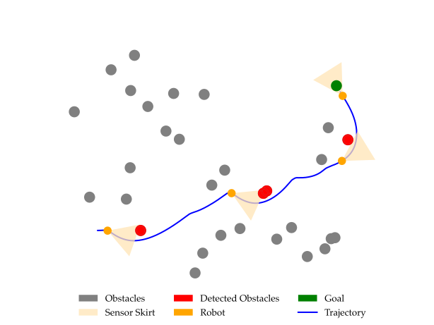
A unicycle with conical sensing follows a known attractor–repulsor navigation policy among randomly positioned obstacles. Each of four viewing-geometry conditions supplies 500 trajectories. Estimated range/angle pairs are close to their generating values: for example, (55, 0.392) becomes (57.037, 0.402). Mean normalized Fréchet distances range from 1.29 to 5.93 in the paper’s reported percentage-like scale, with standard deviations as large as 13.67. These are average path-shape errors, not worst-case guarantees. Four additional 500-trajectory datasets use detection probabilities 0.2, 0.4, 0.6, and 0.8; estimates are 0.2209, 0.4352, 0.6140, and 0.8294. Their corresponding mean normalized distances are 2.55–4.95. A diffusion policy learned from a separate 500-trajectory dataset obtains 3.47±9.31. Testing three unseen viewing geometries yields 7.65–9.79 mean distance over 100 trajectories per condition, with standard deviations of 15.66–20.50. Thus the generalization examples support average resemblance while showing substantial variability. The paper normalizes by start-to-goal distance but does not consistently label table entries as percentages.
Equation 7
| (7) |
| Scenario | Real | Estimated |
|---|---|---|
| 1 | (55, 0.392) | (57.037, 0.402) |
| 2 | (99, 0.785) | (100, 0.826) |
| 3 | (22, 0.523) | (23.063, 0.523) |
| 4 | (70, 0.262) | (71.146, 0.267) |
| Scenario | Normalized Fréchet Distance (Mean Std) |
|---|---|
| 1 | |
| 2 | |
| 3 | |
| 4 |
| Scenario | Actual () | Estimated () |
|---|---|---|
| 1 | 0.2 | 0.2209 |
| 2 | 0.4 | 0.4352 |
| 3 | 0.6 | 0.6140 |
| 4 | 0.8 | 0.8294 |
| Scenario | Normalized Fréchet Distance (Mean Std) |
|---|---|
| 1 | |
| 2 | |
| 3 | |
| 4 |
| Test () | Normalized Fréchet Distance (Mean Std) |
|---|---|
| (80,0.523) | |
| (70,0.785) | |
| (60,0.628) |
IV Imitating Human Behavior
The human study tests joint navigation and gaze-direction imitation in a controlled game. It provides evidence about behavior under an imposed visual restriction, not a direct measurement of natural human visual fields or gaze.
IV-A Godot Game Environment with Data Collection
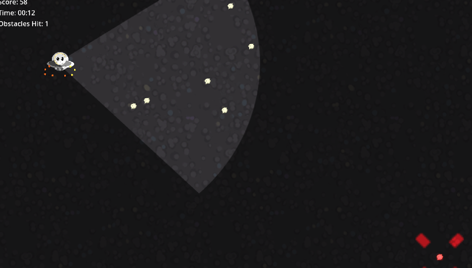
A Godot 4.3 environment collects trajectories while volunteers steer a point-mass agent around stationary and moving obstacles toward a fixed goal.
IV-A 1 Environment Design and Game Mechanics
Keyboard input moves the agent; mouse input independently rotates its viewing direction. Speed limits and obstacles create a tradeoff between reaching the goal quickly and collecting enough visual information. Start and goal locations are fixed within the collection environment.
IV-A 2 Limited Field of View
Only obstacles inside a fixed-range, fixed-angle viewing cone are visible. The goal remains visible throughout the trial. This deliberately simplifies navigation and means that goal localization is not part of the learned perception problem.
IV-A 3 Data Collection
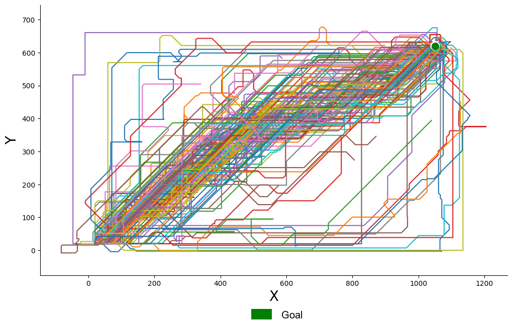
Eight consenting participants supply position and viewing-orientation trajectories, together with logged positions of all static and moving obstacles. The proximity analysis uses 150 human trajectories. The restricted interface and small participant group limit claims about general human navigation, and no participant-held-out evaluation is described.
IV-B Transformer-Based Diffusion for Navigation
A conditional U-Net uses transformer-style multi-head cross-attention to combine noisy actions with observation embeddings. Its outputs are planar displacement and a change in viewing direction. This permits the policy to select where to look while moving, rather than imposing a fixed sensor sweep.
IV-C Trajectory Generation and Validation
Evaluation compares generated and demonstrated paths in the original game, illustrates transfer to scaled laboratory layouts, and measures time spent close to obstacles.
IV-C 1 Original game environment
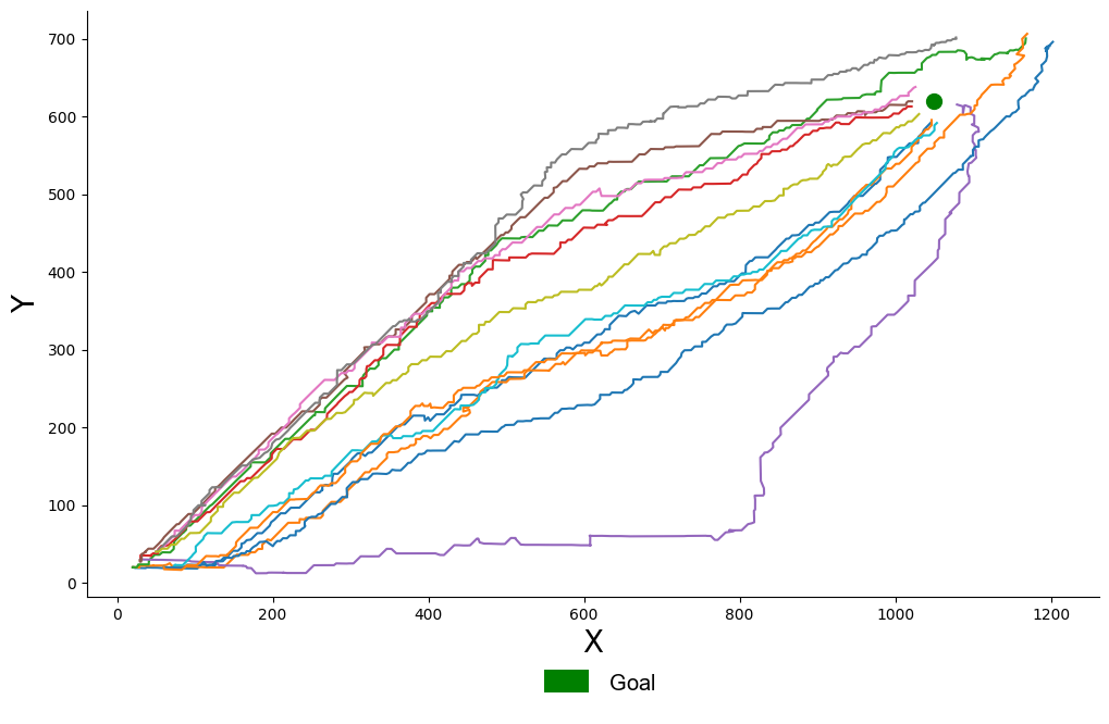
In the original environment, the reported mean normalized Fréchet distance is 11.3±0.06, with a minimum of 4.48. Figure 5 shows human and generated paths in the same layout. The metric assesses geometric path similarity; it does not by itself establish identical attention, intent, or collision behavior. The source does not explain the unusually small uncertainty term or provide a subject-level split.
IV-C 2 Scaled-Down Lab Environment
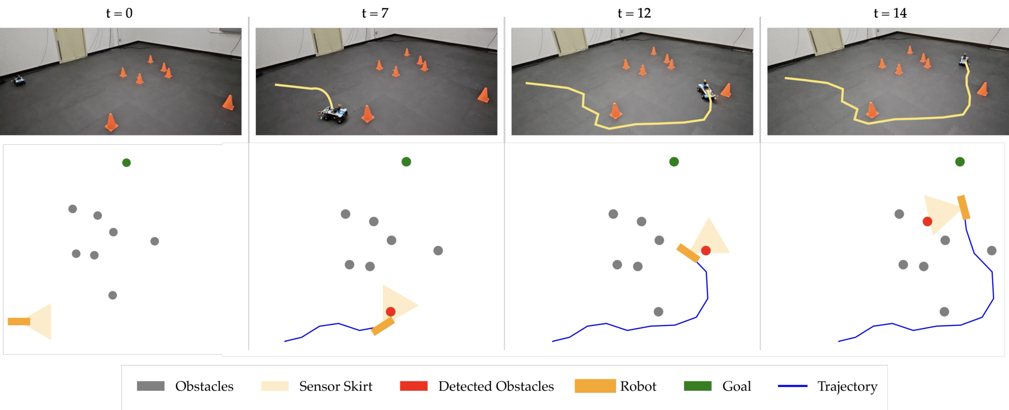
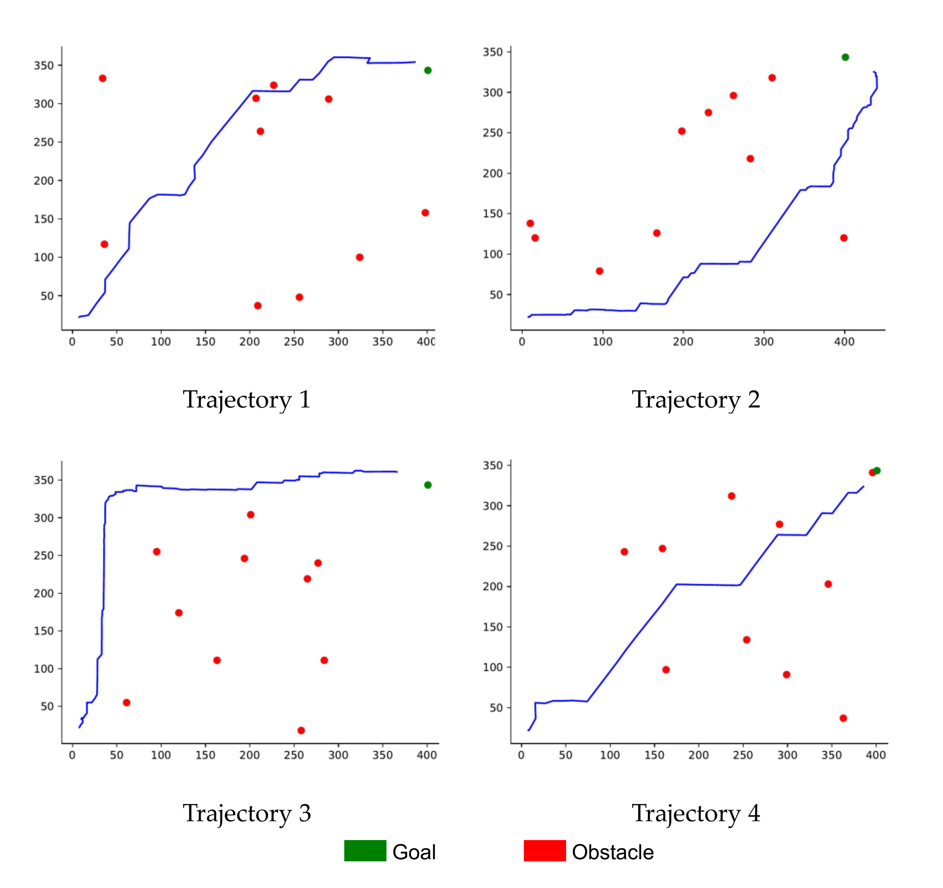
Four previously unseen obstacle layouts illustrate generated routes from the lower-left start to an upper-right goal. These examples demonstrate adaptation of route and sensor direction, but are qualitative examples without aggregate success, collision, or latency statistics.
IV-D Safety Analysis of Trajectories Data
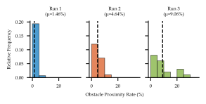
The safety proxy is the fraction of timesteps within 20 game units of any obstacle. Human demonstrations average 1.46%; twenty generated trajectories with learned observation control average 4.64%; twenty baseline trajectories with a fixed sensor angular velocity average 9.06%. Learned viewing reduces proximity by about half relative to this baseline but remains substantially above the human rate. Obstacles retain the collection environment’s movement patterns. The comparison supports the value of adaptive sensor direction under these conditions; proximity is not a collision rate or safety guarantee, and the baseline is not an unrestricted-view optimal planner.
V Hardware Experiment
The hardware demonstration uses a car with bicycle dynamics and independently controlled sensing orientation. Planar policy displacements are converted into speed and heading-error commands with tuned gains. Inference replaces a 100-step diffusion process with ten DDIM steps followed by ten DDPM steps; VICON supplies position and ROS carries commands. Figure 2 shows the car scanning and avoiding static obstacles while reaching its goal. This demonstrates execution with laboratory localization rather than autonomous perception in an uninstrumented environment; repeated-trial performance and measured control latency are not reported. The printed bicycle equations contain notation errors, including a sensor update with the same future-state term on both sides and an omitted timestep in the heading update. They are preserved as published, so the equations should not be copied as an unambiguous controller implementation.
Equations 8–9
| (8) |
| (9) |
VI CONCLUSIONS
Explicitly conditioning imitation on what the demonstrator can see helps explain behavior and supports coordinated movement and sensing. The strongest quantitative human-data result is reduced proximity against fixed sensor rotation. Limits include separately known components during parameter estimation, synthetic constant detection probability, eight game participants, fixed goal visibility and obstacle patterns, variable trajectory errors, and a small instrumented hardware demonstration. Joint identification, broader human studies, stronger sensing baselines, and repeated hardware trials remain open.