At a glance
The paper accelerates repeated motion-planning queries in a fixed graph of convex sets. Offline semidefinite programs construct quadratic lower bounds on remaining path cost; online short-horizon convex lookahead uses those bounds to choose successive regions, with backtracking when necessary. Numerical examples include a simulated seven-joint arm and a 190-vertex graph. The planner trades some path quality for much lower reported solver time, but is incomplete and does not guarantee globally optimal motion in the original free space.
1 Introduction
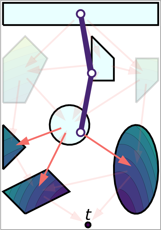
A graph of convex sets [24] represents discrete region choices together with continuous configurations or trajectory parameters. Existing shortest-path formulations [26] optimize both simultaneously, but repeated large mixed discrete–continuous problems can be too slow for an online planning loop.
The proposed approach amortizes work over many queries in an unchanged environment. Convex quadratic value bounds are cheap to store and permit parallel convex lookahead. These bounds guide an approximate policy; they are not a complete precomputed oracle for every optimal path.
1.1 Literature review
Roadmaps and sampling trees search over sampled configurations; GCS searches through continuous collision-free regions, potentially improving path quality while requiring expensive region construction. Classical all-pairs shortest paths and explicit model predictive control motivate precomputing cost-to-go information. Exact value functions can be expensive to compute and represent, so this work chooses inexpensive lower bounds and online lookahead rather than exact dynamic programming.
2 All-Pairs Shortest Paths in a Graph of Convex Sets
The formulation starts with ordinary graph paths, then adds continuous vertex states and convex transition constraints. Its central difficulty is that forbidding repeated vertices makes the optimal continuation depend on the history of visited regions.
2.1 All-Pairs Shortest Paths
The classical graph problem provides the comparison case: fixed nonnegative edge costs allow an optimal successor policy to reconstruct a shortest path from precomputed distances.
Graphs and paths.
A path is a sequence of distinct vertices connected by directed edges. The no-revisit convention matters later: a walk that returns to a convex region at a different continuous state is excluded even if it would reduce total cost.
Shortest Path Problem (SPP).
The ordinary shortest-path problem minimizes summed fixed edge costs. With nonnegative costs, an optimal subpath is itself optimal, supporting a history-independent cost-to-go and efficient dynamic programming.
Equation
All-Pairs Shortest Paths (APSP).
All-pairs shortest paths computes the remaining cost between every source and target vertex. Selecting the outgoing edge with minimum immediate cost plus remaining cost yields the next optimal vertex. A successor table or distance matrix can therefore encode many complete paths compactly.
Equations 1a–1b
| (1a) | ||||
| s.t. | (1b) | |||
2.2 Shortest-Path Problem in a Graph of Convex Sets
GCS replaces each isolated graph node with a convex domain for a continuous optimization variable, and couples neighboring domains through convex costs and constraints.
Graph of Convex Sets.
Each vertex carries a bounded convex set and a variable inside it. Each directed edge restricts the pair of adjacent variables to a convex transition set and assigns a nonnegative convex cost. Selecting a discrete path leaves a continuous convex optimization problem along that path.
The Shortest Path Problem in a Graph of Convex Sets.
The optimization jointly selects a simple vertex path and continuous variables satisfying the prescribed source, target, and transition conditions. Although a fixed path is tractable, selecting the best path is generally NP-hard. Strong mixed-integer convex relaxations and rounding often work well in practice.
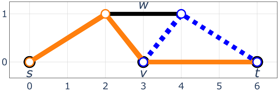
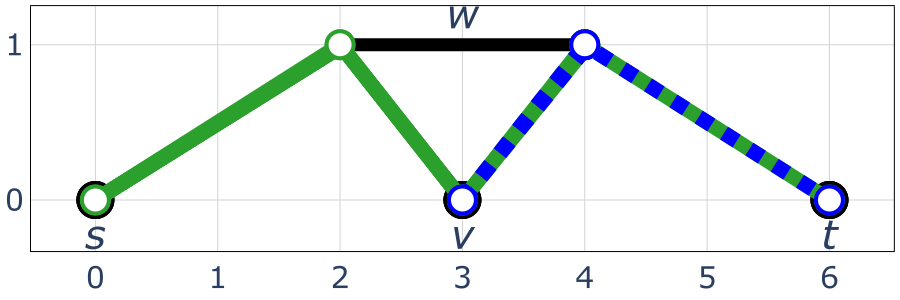
The four-vertex example explains why ordinary Bellman optimality does not transfer directly. A locally optimal continuation may pass through a vertex already visited earlier, invalidating the full simple path. Allowing revisits restores the memoryless principle in this example but changes the requested problem. Thus a value function indexed only by current and target states cannot encode every history-dependent optimal decision.
Equations 2a–2e
| (2a) | ||||||
| s.t. | (2b) | |||||
| (2c) | ||||||
| (2d) | ||||||
| (2e) | ||||||
2.3 All-Pairs Shortest Paths in a Graph of Convex Sets
The multi-query problem asks for paths across specified sets of source and target vertices and every relevant pair of continuous endpoint states. It contains the single-query problem and remains computationally hard.
2.4 Method outline
Offline vertex penalties discourage repeated regions while preserving valid cost lower bounds. Online rollout explicitly excludes previously visited vertices and evaluates several future steps at once to reduce the effect of coarse quadratic bounds. Both the history approximation and the restricted value-function family can introduce suboptimality.
3 Offline phase: synthesis of cost-to-go lower bounds
The derivation first assumes one source region and a fixed target point. It introduces an infinite-dimensional optimization over value functions, then restricts those functions and their certificates to obtain a finite semidefinite program. The appendix extends the construction to multiple sources and continuous or multiple targets.
3.1 Cost-to-go lower bounds via infinite-dimensional LP
The objective raises the average source value under a specified distribution of anticipated starting states. For every feasible transition, a Bellman-like inequality bounds the current value by edge cost, a nonnegative entry penalty for the next vertex, and its remaining value. The terminal value subtracts the sum of all vertex penalties, waiving each penalty once.
The lower-bound proof sums these inequalities along a simple optimal path. Intermediate values telescope; subtracting all penalties cancels every penalty actually accrued and additionally subtracts the nonnegative penalties for vertices never visited. The resulting value is therefore no greater than the true path cost. Those unused penalties also explain a possible relaxation gap: the construction can remain conservative even before choosing quadratic functions.
Equations 3a–5
| (3a) | ||||||
| s.t. | (3b) | |||||
| (3c) | ||||||
| (3d) | ||||||
| (3e) | ||||||
| (4) |
| (5) |
Example 1, continued.
In the four-vertex example, zero penalties give value 14, corresponding to a cheaper walk that revisits a vertex. Optimizing its penalty to 2 recovers the simple-path optimum 16. This example demonstrates possible tightness, not a general equality theorem. When every region is a singleton, the construction reduces to a standard finite shortest-path linear program; general regions require optimization over functions.
Equation 6
| (6) | ||||||
3.2 Numerical approximation via semidefinite programming
Quadratic nonnegativity can be certified through positive-semidefinite matrices. A multiplier certificate enforces nonnegativity on a constrained domain by subtracting a nonnegative combination of its defining inequalities. This S-procedure-style condition is sufficient and can be conservative; restricting value functions and certificates yields a tractable approximation rather than an exact solution of the functional program.
Equation
Defining cost-to-go lower bounds in ( 3b ).
Each lower bound is a convex quadratic with optimized coefficients and a positive-semidefinite curvature constraint. Penalty nonnegativity and the terminal constraint remain linear in the decision variables. The low-order representation keeps evaluation cheap but cannot express a general piecewise value function.
Enforcing the lower-bound constraint ( 3d ).
The numerical construction uses polyhedral or ellipsoidal region and transition descriptions and quadratic edge costs. These assumptions make the transition lower-bound certificate a linear matrix inequality. Nonquadratic costs, including Euclidean distance, are replaced by quadratic approximations, so the certificate must be interpreted for the chosen cost model.
The objective function ( 3a ).
Averaging a quadratic under a fixed source distribution is linear in its coefficients. Higher-degree sum-of-squares bounds could be more expressive but are reported too expensive here. Affine bounds are closely connected to the dual of the standard GCS convex relaxation and provide a cheaper, weaker comparison in the experiments.
4 Online phase: greedy multi-step lookahead policy
At each rollout step, enumerate feasible short vertex sequences that avoid previously visited vertices. Solve their continuous convex lookahead problems in parallel, using actual edge costs and the final quadratic value bound, then execute only the first planned transition. Entry penalties are omitted online because revisits are explicitly prohibited.
Once the target is reached, reoptimize all continuous variables along the selected vertex path. If lookahead becomes infeasible, backtrack to an earlier vertex with another outgoing option. This procedure is sound but incomplete: returned paths satisfy the modeled constraints, but it may fail to find a path that exists. Short-horizon feasibility does not guarantee recursive feasibility, and final continuous reoptimization does not make the discrete path globally optimal.
Equations 7a–7c
| (7a) | ||||
| s.t. | (7b) | |||
| (7c) | ||||
5 Experimental evaluation
All reported experiments are numerical, using a 4.5 GHz sixteen-core Ryzen 9 desktop, 64 GB memory, and Mosek 10.2.1. The evaluation separates a visual two-dimensional example, a simulated arm workload, and a larger graph ablation. Reported online timings use parallelized solver time.
5.1 Two-dimensional example
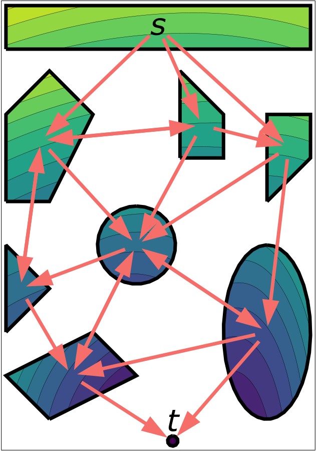
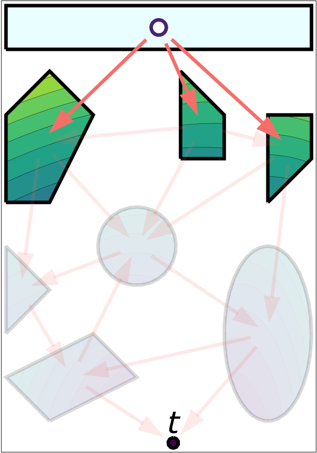
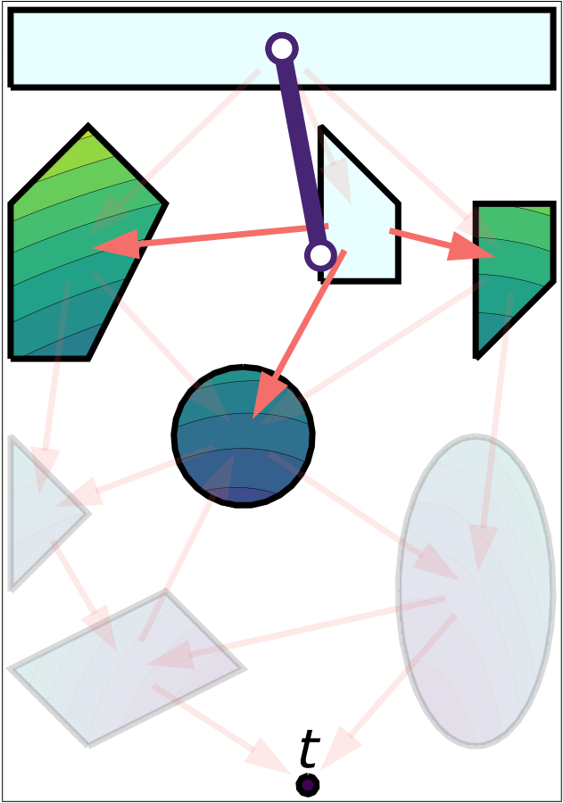
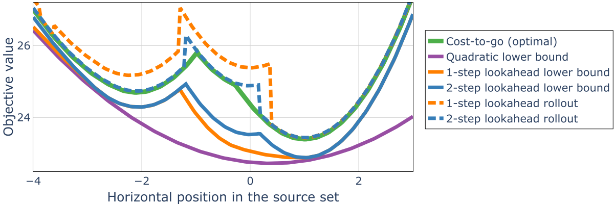
A nine-vertex, twenty-five-edge example uses squared Euclidean edge costs and a point target. Quadratic bounds visibly underestimate the more complex optimal value function. One- and two-step lookahead create more expressive piecewise bounds; two-step rollout is nearly always optimal in the plotted example even though its bound is not everywhere tight. This illustrates the mechanism rather than establishing a general approximation ratio.
5.2 Collision-free motion planning for a robot arm
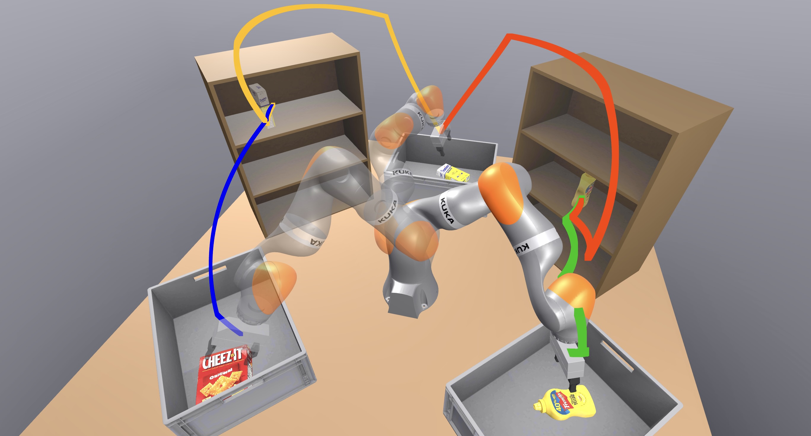
A simulated seven-joint KUKA iiwa moves virtual items between six shelves and three bins. IRIS-NP [29] and clique seeding construct a collision-free convex cover with 23 vertices and 68 edges. Vertices parameterize line segments with position-continuous joins. Twelve source regions and three target regions support 120 queries; bin-to-shelf paths reverse the computed shelf-to-bin solutions.
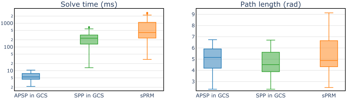
Generating the cover costs about 100 seconds, and the new value bounds add six seconds: Figure 5 reports 106 seconds total offline work for this method, compared with 100 seconds for GCS and 0.9 seconds for the 10,000-vertex shortcut roadmap. The six-second figure alone excludes the shared cover construction.
Online median solver time is 5 ms and maximum 11 ms. The method is reported 40 times faster on average than fresh GCS queries with paths 7% longer, and 110 times faster than shortcut PRM with paths 5% shorter. These are simulated planning results and parallel solver timings, not measured physical-robot control latency. Path quality also depends on the supplied convex cover; no global free-space optimality claim is made.
5.3 Scalability and ablation on lower bounds and lookahead horizon
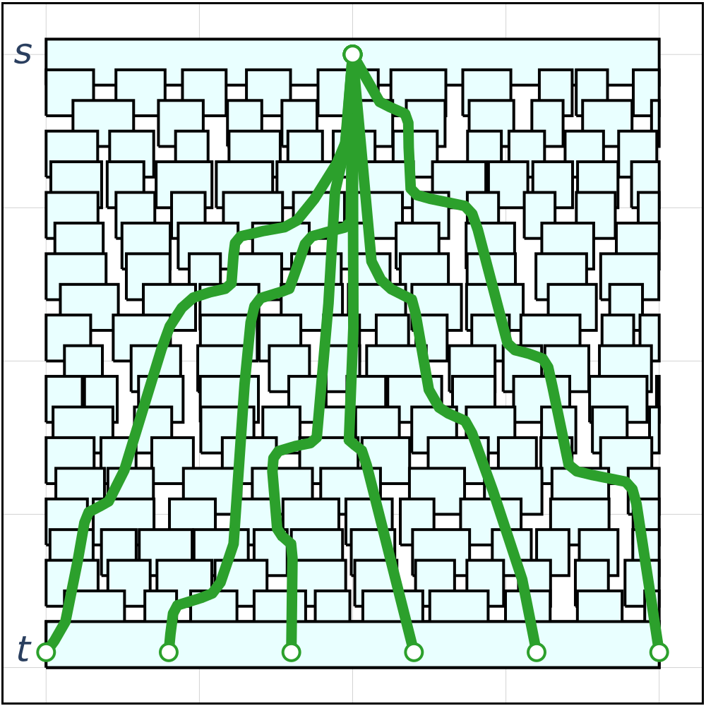
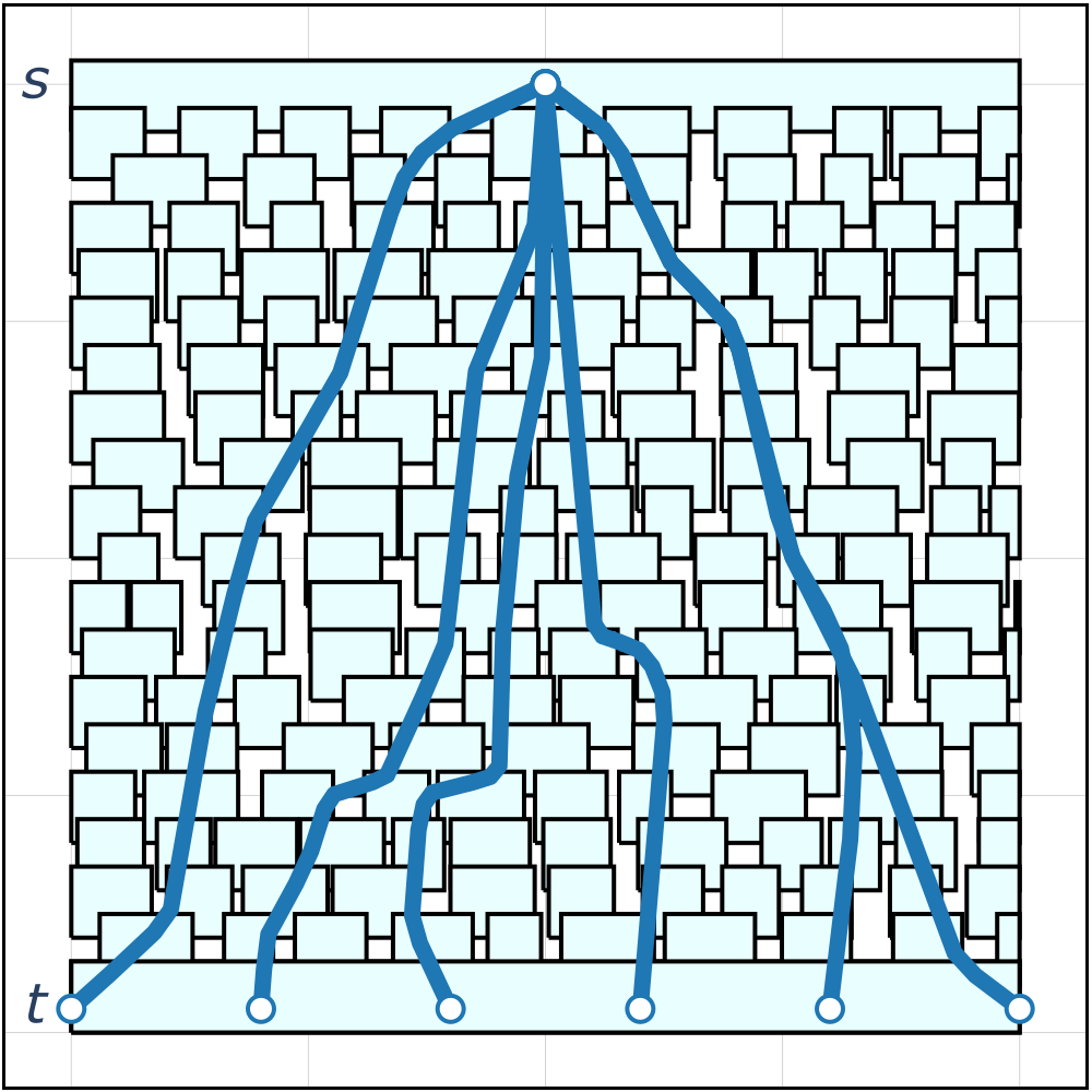
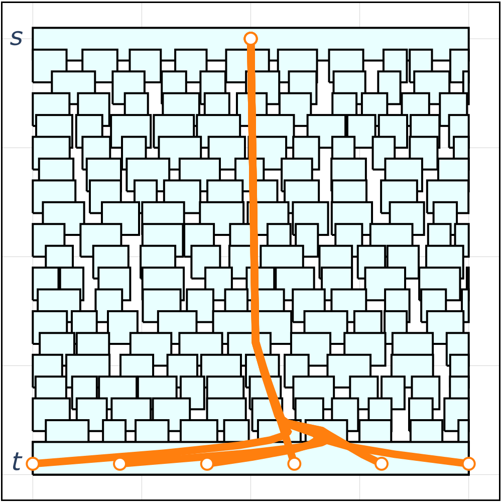
The larger environment has 190 vertices and 540 edges. Vertex variables specify cubic Bézier control points, adjacent curves join with continuous first derivatives, and the objective sums squared control-point distances. Exact mixed-integer solutions supply reference costs for 120 endpoint queries.
Quadratic bounds with two- and three-step lookahead yield median gaps of 9.4% and 8.8% in 4 and 5 ms, with no failures in the tested queries. Affine bounds with three steps yield an 80.2% median gap and 9.9% failures; nine steps improve the gap to 7.0% but take 388 ms. Rollouts stop after 10,000 iterations, so failure rates reflect that finite budget.
Table 1 reports a 6.9% median gap and 716 ms median time for the standard GCS relaxation-based planner; its 75th-percentile time is 1,051 ms. This distinguishes the table statistics from prose describing time above 1,000 ms. Observing no failures for selected quadratic settings does not make the incomplete algorithm complete.
| Solution method | Optimality gap, % | Solve time, ms | Failure rate, % |
| Quadratic , 1-step | 20.0 (62.1) | 3 (3) | 0.0 |
| Quadratic , 2-step | 9.4 (22.3) | 4 (4) | 0.0 |
| Quadratic , 3-step | 8.8 (15.7) | 5 (6) | 0.0 |
| Affine , 1-step | 157.1 (N/A) | 2 (657) | 27.2 |
| Affine , 2-step | 142.4 (418.8) | 3 (914) | 14.0 |
| Affine , 3-step | 80.2 (348.3) | 5 (808) | 9.9 |
| Affine , 8-step | 11.9 (37.4) | 169 (1996) | 3.3 |
| Affine , 9-step | 7.0 (26.2) | 388 (2454) | 0.0 |
| SPP in GCS | 6.9 (12.0) | 716 (1051) | 0.0 |
6 Conclusion and future work
The results support amortizing static-environment planning through quadratic cost bounds and short convex lookahead. Remaining limits include expensive convex-cover construction, approximate costs and value functions, history dependence, and incomplete online search. Moving obstacles, grasp-dependent geometry, and alternative search policies are future work. Adding nonconvex online constraints could accommodate changes but would alter the convex-solver advantage tested here.
Appendix 0.A Extensions and variations
Multiple source regions contribute additional average-value terms to the objective. A continuous target region is handled by value functions of both current and target states, with corresponding transition and terminal constraints. Target-dependent nonnegative penalties can tighten the bounds, and separate programs for multiple target vertices can run in parallel.
The online policy likewise receives the target vertex and point. The appendix also proposes penalties for traversing both directions of a two-cycle, waived once at the target, and sketches extension to longer cycles. These variations retain the lower-bound construction’s intent; they do not supply a general completeness or exact-optimality guarantee.
Equations
| s.t. | |||