Overview
The paper studies how explicit concept schemas can help interpret unconventional visual representations of familiar abstractions.
At a glance
Deep Schema Grounding uses a language model to decompose a named abstract concept into dependent components, then queries a vision-language model to ground those components in an image before answering questions. The Visual Abstractions Benchmark contains 540 questions over 180 images and twelve concepts. With GPT-4o, the method improves multiple-choice exact-match accuracy from 66.4% to 73.0%. It is an inference-time prompting framework, not a newly trained vision model, and it remains limited by ambiguous schemas and visual grounding errors.
1 Introduction
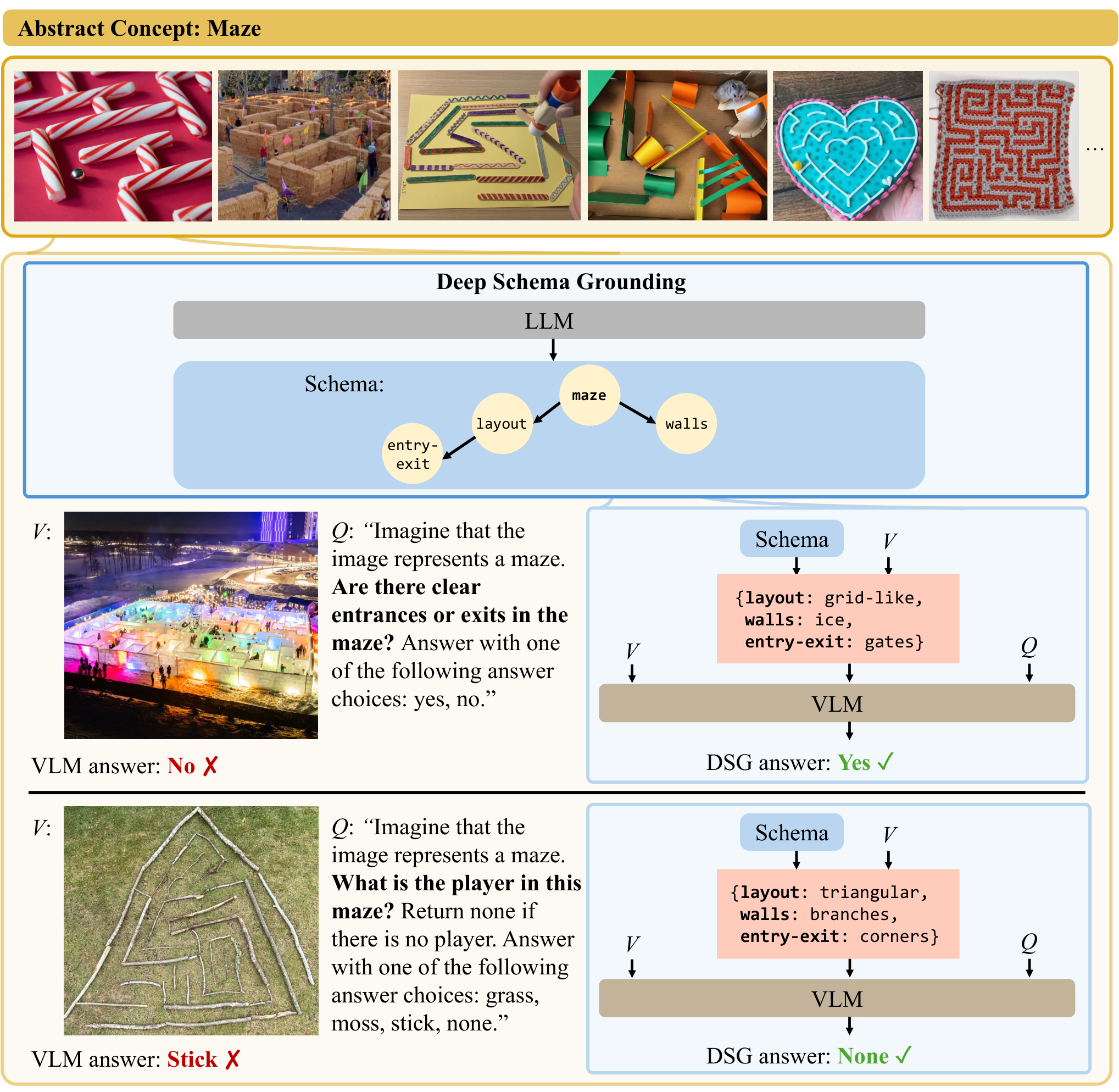
A maze can be made from drawn lines, food, or household objects. Recognizing the material alone does not identify its role as walls, layout, or entry and exit. The proposed framework supplies a structured decomposition of an already named concept and uses its dependencies to guide visual interpretation. It aims to improve reasoning across different instantiations; discovering the intended concept from an unlabeled image is outside the evaluated task.
2 Related Works
The work connects visual question answering, cognitive accounts of concepts, and hierarchical visual reasoning.
Vision-language grounding and reasoning benchmarks.
Existing benchmarks examine objects, relations, commonsense questions, and scene descriptions. This benchmark focuses on visual instantiations of abstract concepts, where low-level entities must be interpreted according to a higher-level pattern.
Concept representations in minds and machines.
The schema view draws on cognitive theories treating concepts as structured explanatory knowledge, including Schank and Abelson’s scripts and plans. Here, that inspiration becomes a dependency graph used to guide model queries; the experiments do not establish a mechanistic match to human cognition.
Hierarchical grounding of visual concepts.
Prior methods use intermediate reasoning, class descriptions, hierarchies, and executable programs. This method instead grounds a language-generated concept graph through repeated visual-model queries. Its inference remains model-based natural-language interpretation, rather than a symbolic engine that guarantees logically correct results.
3 Deep Schema Grounding
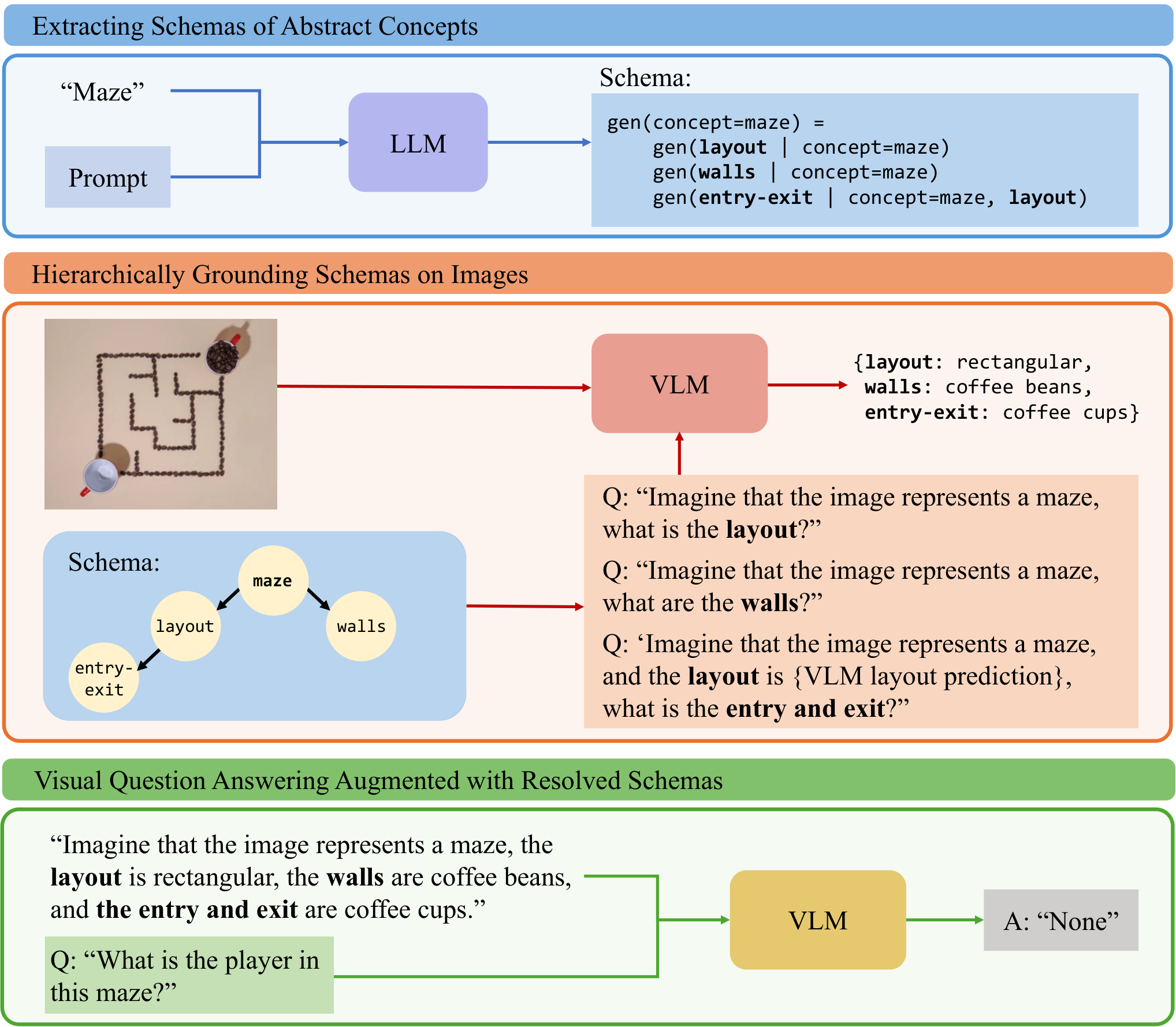
The input is an image and a question that explicitly reveals its intended abstract concept to every method. The pipeline extracts a schema, grounds its components in dependency order, and supplies the resolved schema to the final answering model. No task-specific parameter training is performed.
3.1 Visual Abstraction Schema
A schema is a concise program-like description of a directed acyclic graph. Nodes denote components such as maze layout, walls, and entry/exit; edges determine which earlier interpretations condition a later one. The schema is intended to generalize across materials and scenes, but its claimed universality is an intended property, not formally verified.
3.2 Extracting Schemas of Abstract Concepts
A language model receives a simple schema-generation instruction and one example based on academia. It proposes a decomposition from the concept’s name without seeing the individual target image. The appendix preserves the exact prompt and all twelve resulting schemas, including the instruction to use at most four necessary visually mappable components.
3.3 Hierarchically Grounding Schemas on Images
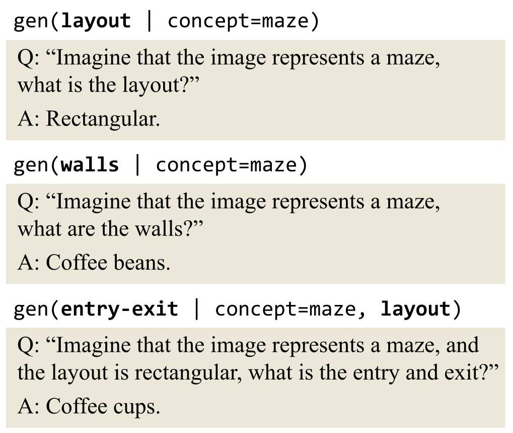
The vision-language model first describes components without prerequisites, then grounds dependent components using those earlier descriptions. For a maze, the identified layout can inform the interpretation of entries and exits. Outputs are short language descriptions rather than verified object masks or geometric constraints. Incorrect early descriptions can therefore influence later grounding.
3.4 Visual Question-Answering Augmented with Grounded Schemas
The final model receives the original image and question, component mappings, and the grounding conversation history. This gives it richer image-derived context than the concept name alone. The approach trades extra model queries and context for more explicit reasoning; the paper does not supply a measured latency or monetary-cost comparison.
4 Visual Abstractions Benchmark
The Visual Abstractions Benchmark contains fifteen images per concept, twelve concepts, and three questions per image: 180 images and 540 question–image pairs. It is a small, manually curated test set, with additional free-response evaluation.
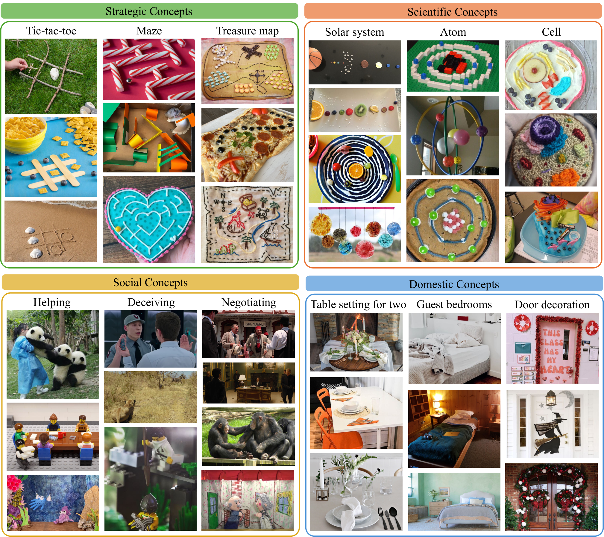
Abstract concepts.
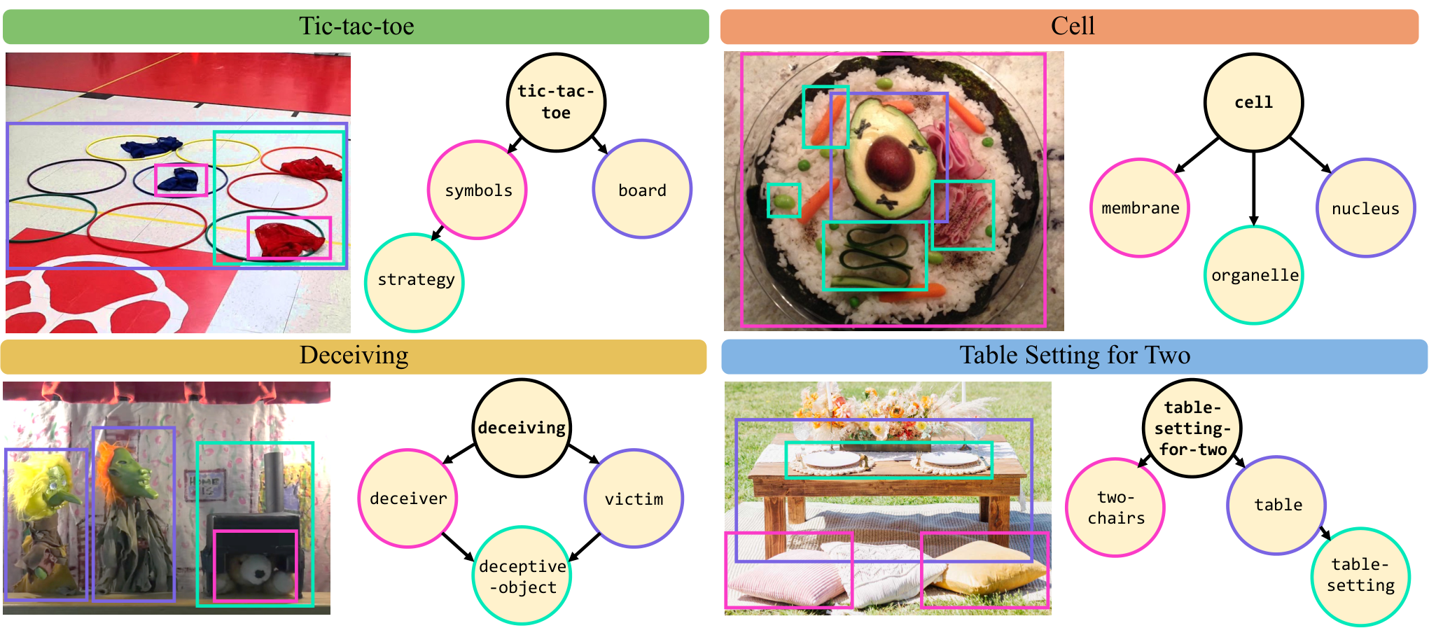
Four concept groups are represented: strategic games such as mazes and tic-tac-toe; physical constructions illustrating scientific ideas such as atoms and cells; social situations such as helping or deceiving; and household goals such as setting a table for two. These groups require different forms of relational interpretation and are not interchangeable difficulty levels.
Images and question-answers.
Images come from the internet and are chosen for varied real-world instantiations. Questions cover binary choices, counts, and more general content. In the main evaluation, all question categories—including those called open-ended—use multiple-choice answers scored against the modal response of five annotators. The separate free-response variant uses different metrics.
5 Results
Baselines include visual models and language models that call visual tools. Every method receives the intended concept. Reported main results average five runs on the same benchmark; these repetitions measure run variability, not performance across five independent datasets.
| All | Counting | Binary | Open | |
| ViperGPT (Surís et al., 2023) | ||||
| VisProg (Gupta & Kembhavi, 2023) | ||||
| LLaVA (Liu et al., 2024) | ||||
| InstructBLIP (Dai et al., 2024) | ||||
| GPT-4o (OpenAI, 2024) | ||||
| DSG (ours) | ||||
| Human |
| Strategic | Scientific | Social | Domestic | |
| GPT-4o (OpenAI, 2024) | ||||
| DSG (ours) |
VLMs benefit from decomposing abstract concepts into primitive-level components.
GPT-4o accuracy rises from 66.4% to 73.0%, a 6.6-percentage-point gain. Counting rises from 60.4% to 70.4%, binary questions from 65.5% to 69.0%, and the open-content multiple-choice category from 69.3% to 77.6%. Gains occur in all four concept groups, with the largest in strategic concepts. A randomly chosen human annotator agrees with the modal label 84.6% of the time, showing both remaining model headroom and imperfect annotator agreement; this is not an independently adjudicated upper bound. The older GPT-4v also improves from 65.3% to 70.7% under the framework.
Explicit hierarchical grounding of schemas is better than implicit and sequential grounding.
Adding a schema in one prompt reaches 68.1%; sequential explicit grounding reaches 69.3%; hierarchical grounding without full conversation history reaches 70.1%; the full pipeline reaches 73.0%. These ablations support the combined design on average, but individual categories do not improve monotonically: sequential grounding has higher counting accuracy than the full method. The comparisons do not isolate structured reasoning from the additional inference work in a cost-matched experiment.
DSG improves other (open-source) VLMs, too.
With LLaVA as the visual model, accuracy increases from 41.5% to 44.4%, or about 7% relative. Counting remains unchanged at 34.4%. The method can help more than one model, but cannot compensate fully for a base model’s weak counting or perception.
| All | Counting | Binary | Open | |
| LLaVA (Liu et al., 2024) | ||||
| DSG (ours) |
| Strategic | Scientific | Social | Domestic | |
| LLaVA (Liu et al., 2024) | ||||
| DSG (ours) |
6 Discussion
Generated schemas can be biased, ambiguous, or unsuitable for particular images. Precise spatial components are especially difficult: naming an unobstructed maze path does not equip the visual model to verify that path. The flexible language interface avoids a fixed vocabulary but provides no formal grounding guarantee. Better layouts, component grounding, and more efficient inference remain open problems; the method is not a general solution to abstraction or spatial reasoning.
7 Conclusion
Explicit concept decomposition and dependency-aware visual grounding improve the tested question-answering systems. The main contribution is a reusable inference procedure and benchmark, with evidence of benefits across several concepts and models while substantial errors remain.
Acknowledgments
The authors acknowledge feedback and support from university, government, and industry research programs, plus individual fellowship support.
Supplementary for: What Makes a Maze Look Like a Maze?
The supplement adds evaluation metrics and ablations, qualitative grounding examples, benchmark construction details, the full prompts and schemas, and a human assessment of schema quality.
Appendix A Additional Results
Additional results examine answer ambiguity, free responses, query structure, image access, and schema complexity.
A.1 Graded Accuracy Comparison
The graded metric awards the fraction of five annotators who agree with a prediction, rather than requiring agreement with the modal answer. GPT-4o scores 0.622 and the proposed method 0.684. This preserves the main trend while acknowledging label disagreement; it measures alignment with this annotator set, not objective correctness independent of interpretation.
| All | Counting | Binary | Open | |
| ViperGPT (Surís et al., 2023) | ||||
| VisProg (Gupta & Kembhavi, 2023) | ||||
| LLaVA (Liu et al., 2024) | ||||
| InstructBLIP (Dai et al., 2024) | ||||
| GPT-4o (OpenAI, 2024) | ||||
| DSG (ours) | ||||
| Human |
A.2 Comparison on Free Response Generation
Free-response BERTScore increases from 0.900 to 0.908, a small change in text similarity rather than an accuracy percentage. Using the GPT-4 answer-evaluation protocol, overall scores rise from 36.67 to 37.78. Counting and open-response scores improve, while binary scores fall from 55.24 to 49.52. Model-judged answers and similarity metrics have different limitations from exact-match evaluation.
| All | Counting | Binary | Open | |
| GPT-4o (OpenAI, 2024) | ||||
| DSG (ours) |
| All | Counting | Binary | Open | |
| GPT-4o | ||||
| DSG (ours) |
A.3 Results on Single-round vs. Multi-round Reasoning
One-query prompts containing schema components or the full hierarchy obtain 66.7% and 68.1%, compared with 73.0% for explicit multi-round grounding. The result supports separate grounding steps for the tested models, while leaving their additional query cost and whether other single-query prompts could close the gap unresolved.
A.4 Language-only Baselines
Removing image access entirely gives 39.7% accuracy. Supplying a previously image-grounded schema to the final language-only answer step raises this to 52.2%. The latter is not a purely text-only pipeline: its schema already contains visual information. Full visual access and grounding together remain better.
A.5 Schema Complexity Ablation
Examples with three, five, seven, or nine components produce overall accuracies of 73.0%, 69.1%, 68.5%, and 67.6%. The more detailed examples yield average generated schema lengths of 3.00, 4.66, 5.75, and 7.00 components. Longer schemas can introduce harder or less general components; the evidence does not show that future stronger models will necessarily benefit from adding detail. All four original example programs are retained with their source indentation.
With 3 components:
gen(concept=academia) =
    gen(faculty | concept=academia)
    gen(students | concept=academia)
    gen(research-output | concept=academia, faculty, students)
With 5 components:
gen(concept=academia) =
gen(faculty | concept=academia)
gen(students | concept=academia)
gen(courses | concept=academia, faculty, students)
gen(research-output | concept=academia, faculty, students, courses)
gen(funding | concept=academia, research-output)With 7 components:
gen(concept=academia) =
gen(faculty | concept=academia)
gen(students | concept=academia)
gen(departments | concept=academia, faculty, students)
gen(courses | concept=academia, departments, faculty, students)
gen(research-output | concept=academia, departments, faculty, students)
gen(funding | concept=academia, research-output, departments)
gen(infrastructure | concept=academia, funding, departments, courses)With 9 components:
gen(concept=academia) =
gen(faculty | concept=academia)
gen(students | concept=academia)
gen(departments | concept=academia, faculty, students)
gen(courses | concept=academia, departments, faculty, students)
gen(research-output | concept=academia, departments, faculty, students)
gen(funding | concept=academia, research-output, departments)
gen(infrastructure | concept=academia, funding, departments, courses)
gen(administration | concept=academia, infrastructure, departments, faculty, students)
gen(community-engagement | concept=academia, research-output, administration, students, faculty)| All | Counting | Binary | Open | |
| DSG w/ 3 comp. | ||||
| DSG w/ 5 comp. | ||||
| DSG w/ 7 comp. | ||||
| DSG w/ 9 comp. |
| Generated comp. # | |
| 3 comp. | |
| 5 comp. | |
| 7 comp. | |
| 9 comp. |
A.6 Qualitative Examples
The retained examples show grounded schemas across concept groups, with incorrect component interpretations highlighted in red. They illustrate how errors can persist despite a sensible high-level decomposition and should be read alongside the quantitative averages.
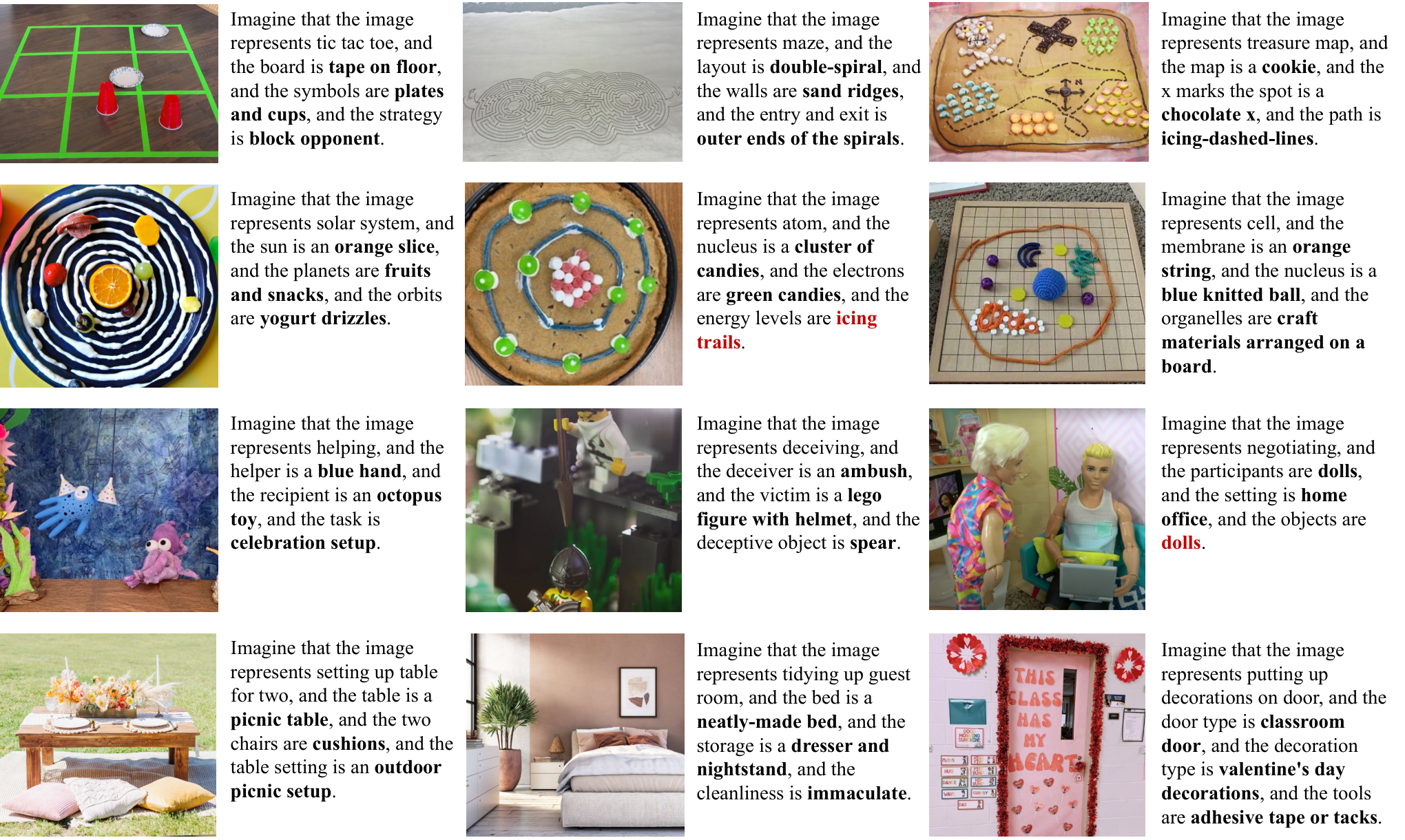
A.7 Hierarchical Grounding Example
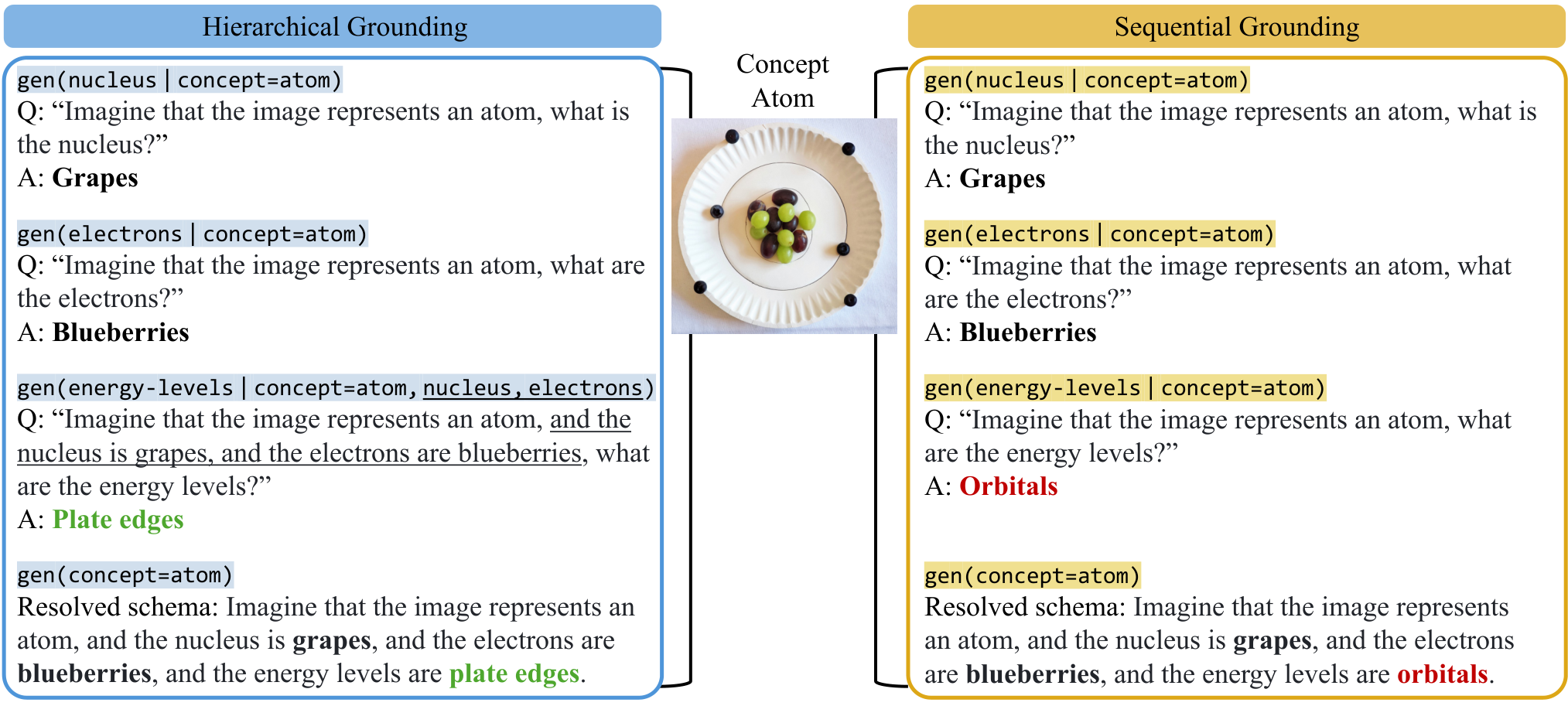
An atom example contrasts hierarchical grounding with a sequential variant. Conditioning energy-level interpretation on previously grounded nucleus and electron descriptions produces a better interpretation in that example. This is qualitative support for dependency ordering, not a separate broad accuracy estimate.
A.8 Computing Resources
Closed-model experiments use the OpenAI interface. Open models and visual-tool components run inference on one A40 accelerator. No model training is required by the framework, but multiple calls per example still contribute inference cost.
Appendix B Visual Abstractions Benchmark
The benchmark appendix documents images, questions, selection criteria, annotations, and release organization.
B.1 Benchmark Examples
The complete retained montage provides question–image pairs across all concept and question categories, complementing the main overview of the twelve concepts.
B.2 Benchmark Construction
Researchers manually search for diverse physical instantiations of each concept and select faithful, high-quality images. They write broadly applicable questions and send the resulting pairs for annotation. This selection process is not procedurally reproducible and can shape which kinds of abstraction the benchmark tests.
B.3 Annotation
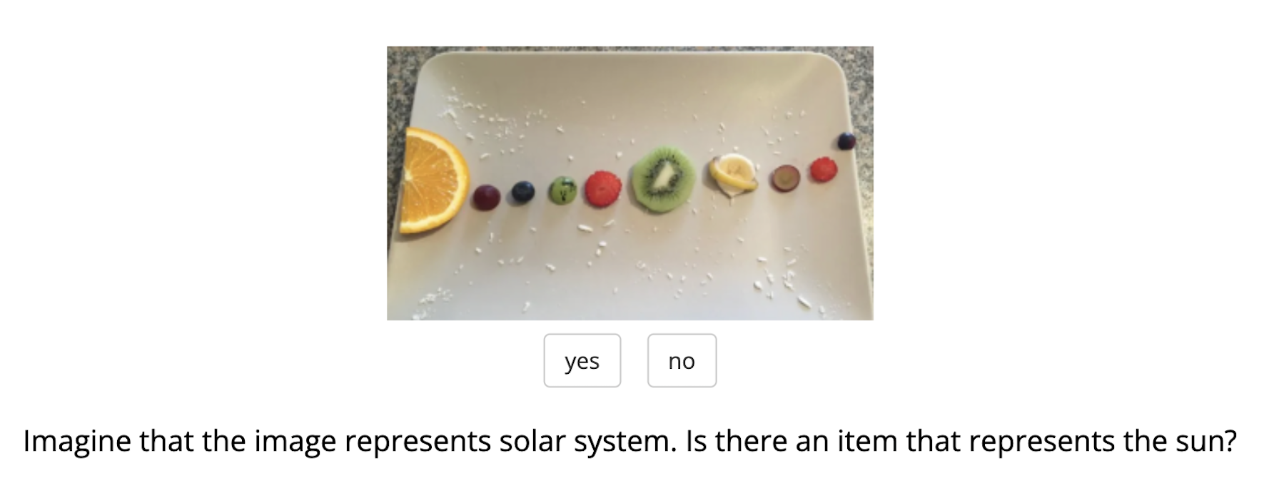
Five Prolific annotators label each question–image pair through the illustrated interface, with compensation stated as twelve US dollars per hour. Their modal response defines the primary evaluation label; disagreement motivates the graded supplementary metric.
B.4 Release
The released benchmark groups images by concept. The paper reports manual auditing of the release. This is the benchmark evaluated here, rather than an automatically sampled distribution of all possible visual abstractions.
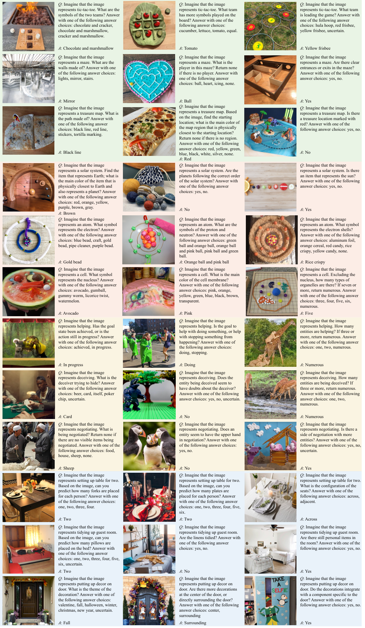
Appendix C LLM-Generated Schemas
The final appendix makes the schema-generation prompt, all twelve extracted schemas, and the schema-quality study available for inspection.
C.1 Prompt
The exact original prompt asks for a simple program-like concept schema, supplies an academia example, requests the same format without explanation, and limits the output to four or fewer necessary components that can map to image objects. Its examples and formatting are preserved below.
Can you give me a program representing the schema for a concept? For example,
gen(concept=academia) =
    gen(faculty | concept=academia)
    gen(students | concept=academia)
    gen(research-output | concept=academia, faculty, students)
Please do the same for gen(concept=[abstract-concept]) in the same format without explanation. Keep the program simple with four or less components. Use only the most necessary parts of the schema that can be mapped to objects in an image.
C.2 All Schemas
All original schemas are retained by strategic, scientific, social, and domestic category. Their component names and conditional dependencies define the structure actually supplied to the grounding procedure, making omissions and potentially ambiguous concepts visible.
gen(concept=tic-tac-toe) =
    gen(board | concept=tic-tac-toe)
    gen(symbols | concept=tic-tac-toe)
    gen(strategy | concept=tic-tac-toe, symbols)

gen(concept=maze) =
    gen(layout | concept=maze)
    gen(walls | concept=maze)
    gen(entry-exit | concept=maze, layout)

gen(concept=treasure-map) =
    gen(map | concept=treasure-map)
    gen(x-marks-the-spot | concept=treasure-map)
    gen(path | concept=treasure-map, map)
gen(concept=solar-system) =
gen(sun | concept=solar-system)
gen(planets | concept=solar-system)
gen(orbits | concept=solar-system, sun, planets)
gen(concept=atom) =
gen(nucleus | concept=atom)
gen(electrons | concept=atom)
gen(energy-levels | concept=atom, nucleus, electrons)
gen(concept=cell) =
gen(membrane | concept=cell)
gen(nucleus | concept=cell)
gen(organelles | concept=cell)gen(concept=helping) =
gen(helper | concept=helping)
gen(recipient | concept=helping)
gen(task | concept=helping, helper, recipient)
gen(concept=deceiving) =
gen(deceiver | concept=deceiving)
gen(victim | concept=deceiving)
gen(deceptive-object | concept=deceiving, deceiver, victim)
gen(concept=negotiating) =
gen(participants | concept=negotiating)
gen(setting | concept=negotiating)
gen(objects | concept=negotiating, participants)gen(concept=setting-up-table-for-two) =
gen(table | concept=setting-up-table-for-two)
gen(two-chairs | concept=setting-up-table-for-two)
gen(table-setting | concept=setting-up-table-for-two, table)
gen(concept=tidying-up-guest-room) =
gen(bed | concept=tidying-up-guest-room)
gen(storage | concept=tidying-up-guest-room)
gen(cleanliness | concept=tidying-up-guest-room, bed, storage)
gen(concept=putting-up-decorations-on-door) =
gen(decoration-type | concept=putting-up-decorations-on-door)
gen(door-type | concept=putting-up-decorations-on-door)
gen(tools | concept=putting-up-decorations-on-door, decoration-type)C.3 Human Study of Schema Quality
Twenty participants judge twelve schemas on representativeness, components to keep, and components to add, producing 720 answers. Mean representativeness is 5.74 out of seven; participants retain 2.59 of the three components on average and suggest 1.59 additions. Negotiating receives the lowest mean representativeness and component-retention scores. These judgments support reasonable initial schemas while showing incompleteness; they do not verify every grounding or prove universal concept definitions.
Here you are given a concept, maze, and the core components underlying it: layout, walls, entry-exit. How well do these core components represent this concept on a scale of 1-7?
Here you are given a concept, maze, and the core components underlying it: layout, walls, entry-exit. How many components out of the ones listed accurately represent part of this concept?
Here you are given a concept, maze, and the core components underlying it: layout, walls, entry-exit. How many more components, if any, would you add to accurately represent this concept?
| Representativeness (1-7) | # comp. to keep | # comp. to add | |
| Participant responses |