At a glance
Robust Robot Walker trains a Unitree A1 quadruped to cross small bars, pits, and poles using proprioception at deployment. Simulation supplies privileged contact forces, velocity, friction, and trap labels to train a contact representation and a recurrent estimator. A second stage gradually replaces privileged information with estimates.
The method combines dense goal-tracking rewards with constant, artificial goal commands for teleoperation. It reaches 93.4% success on a mixed simulated trap course and demonstrates physical recovery from several trap types. The controller reacts after contact rather than visually anticipating hazards. Its approximate omnidirectional interface cannot independently command speed magnitude, and highly deformable traps remain difficult.
Task overview
The task is reactive traversal of bars, pits, and poles using the robot’s own state rather than camera input.
I INTRODUCTION
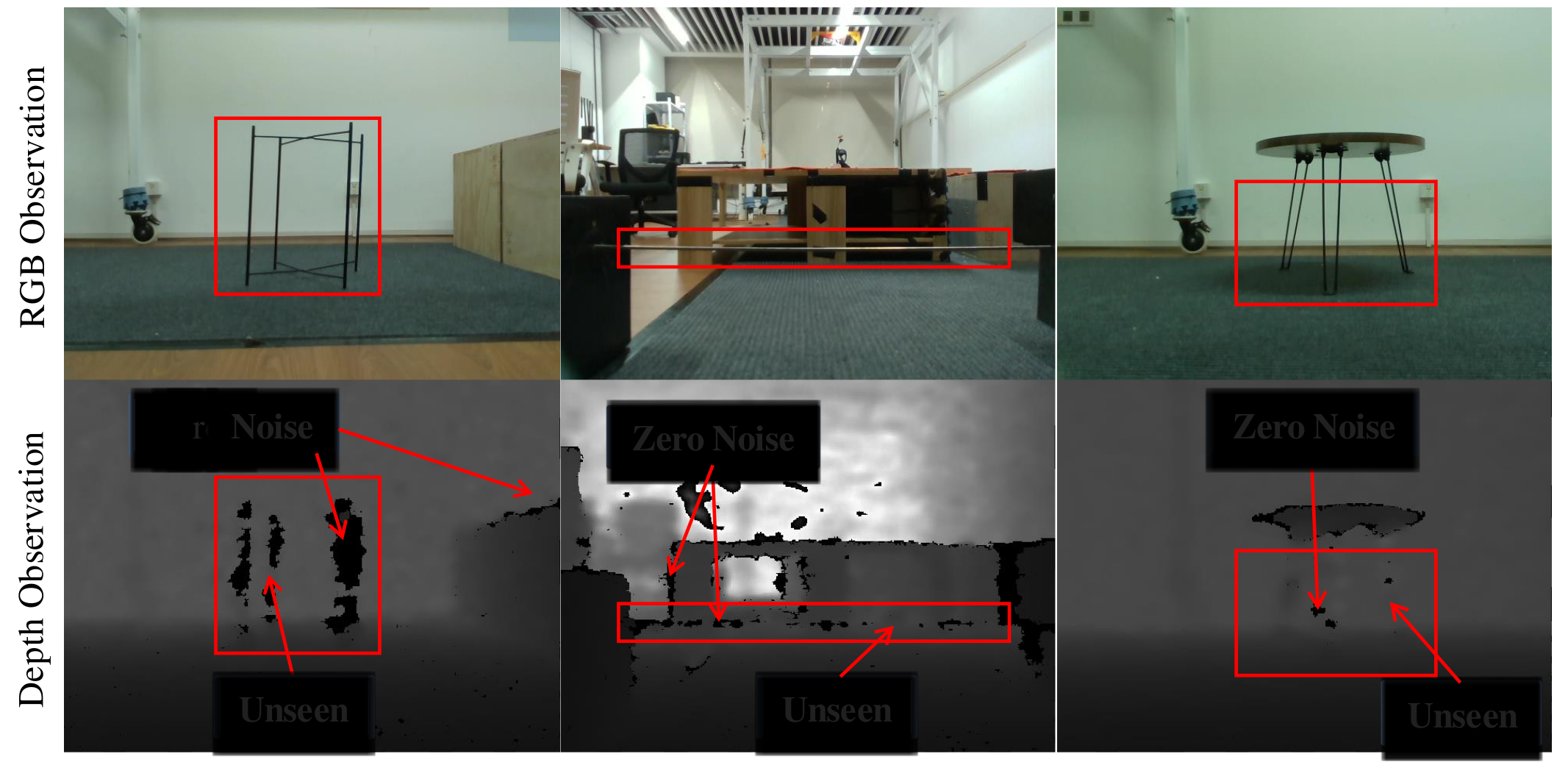
Thin or occluded hazards can be unreliable in depth images and may lie below or behind the camera. The proposed response is to infer contact consequences from the robot’s own motion and joint signals. Figure 2 illustrates depth-sensing failures; it does not imply that all external perception is ineffective.
The key components are a learned contact-force latent, trap-class supervision during training, probability-annealed replacement of privileged state, and dense goal-tracking rewards. Artificial goal vectors turn the trained goal policy into a joystick-controlled movement policy without motion capture or external localization.
II RELATED WORKS
The method builds on reinforcement-learning locomotion and learned contact estimation, combining them for small hazards that the robot encounters before it can react.
II-A Learning-Based Locomotion
Prior learned controllers cover uneven terrain, stairs, parkour, and manipulation with legs. Goal-driven locomotion and agile blind locomotion motivate the task formulation here. The contribution targets trap recovery and deployment commands, rather than proposing reinforcement learning for locomotion itself.
II-B Collision Detection
Collision handling includes detection, localization, force identification, classification, and reaction. Model-based observers infer contact from dynamics; model-free methods learn explicit contact states or implicit representations. The comparison with Boolean collision prediction motivates a continuous contact-force latent, though its transfer benefit is assessed within this training system.
III METHOD
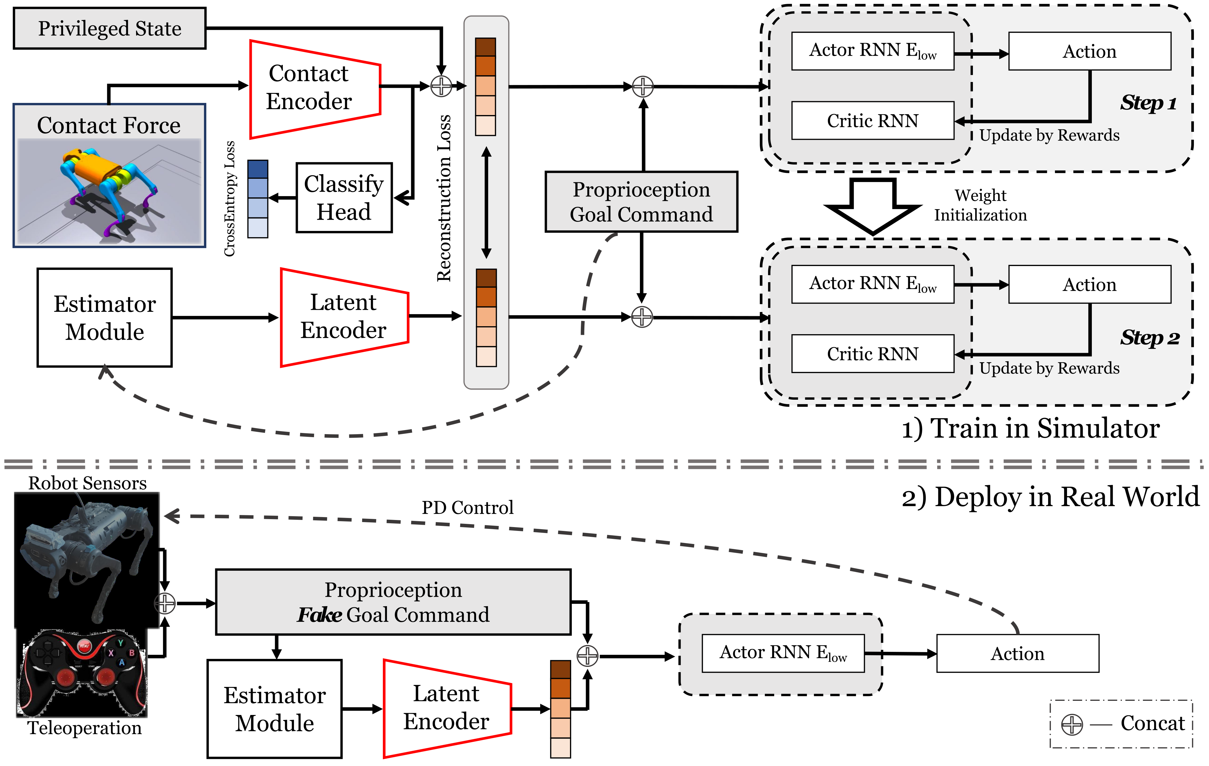
Training first exposes the policy to privileged simulation signals, then adapts it to a recurrent state estimate. Deployment retains only proprioception, recurrent memory, and operator commands.
III-A Task Definition
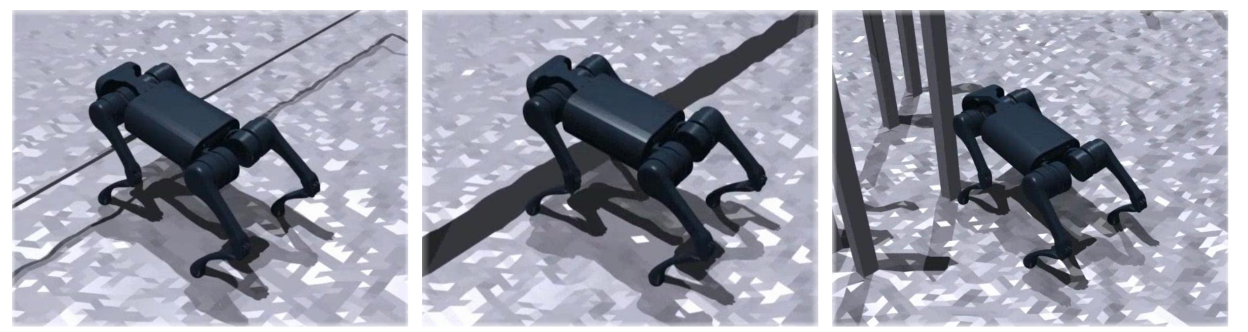
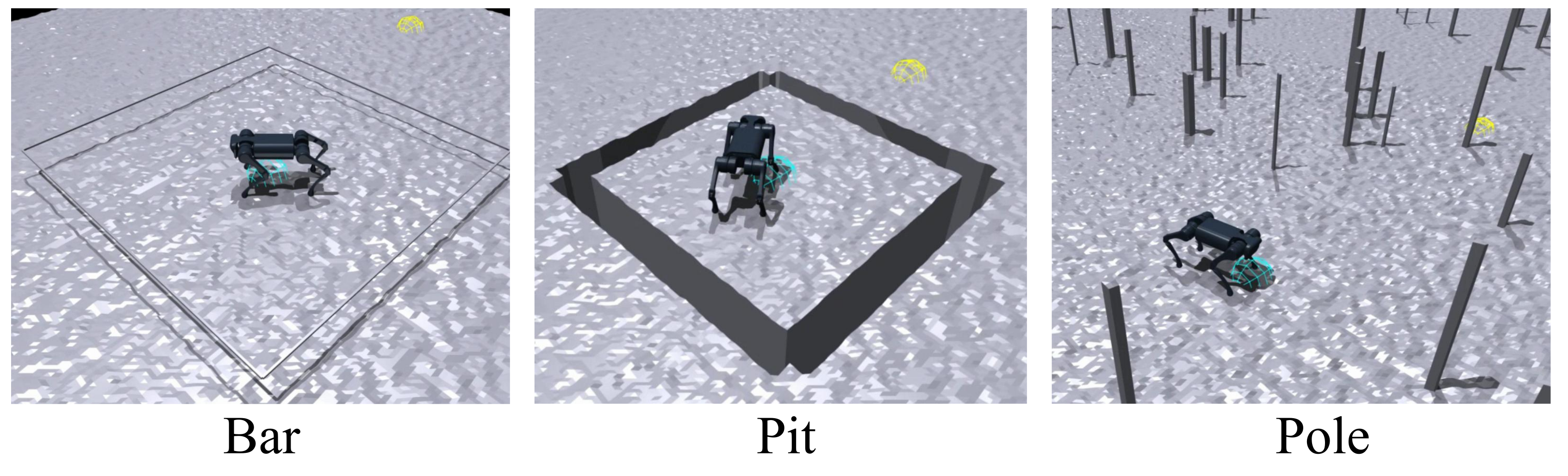
Bars are horizontal obstacles below head height, pits are depressions that catch a foot, and poles are thin upright obstacles. The robot must pass them under constant commands while adapting its own motion. Both thin and thicker obstacles appear in the evaluation; the thicker ones also test behavioral generalization even when a camera could detect them.
III-B Reinforcement Learning Setting
PPO controls twelve desired joint positions every 0.02 seconds. Proprioception contains gravity direction, base angular velocity, joint positions and velocities, and the previous action. Training additionally provides base linear velocity, ground friction, and clipped/normalized contact forces for the robot links.
A training command specifies a goal displacement in the robot frame and remaining episode time. The world-frame goal stays fixed while its relative displacement updates with robot motion; vertical displacement is zero. Within 0.2 m, the displacement is set to zero to train stopping. Deployment replaces this evolving localization-dependent command with constant artificial values.
III-C Reward Function
The task reward increases densely as distance to the goal shrinks. A heading term encourages facing the goal, simplifying trap learning mainly to forward or slightly angled approaches. Near the goal, negative-weight finish terms penalize joint deviation from the default pose and residual linear/angular speed.
Regularization discourages stalling and excessive motion while encouraging stable, smooth gait; an adversarial motion prior adds a style reward. Table III retains every formula and weight. The velocity-limit term is a training incentive, not a hard safety constraint. Its source expression uses signed yaw velocity rather than absolute yaw speed; the formula is preserved as printed.
Equations 1–6
| (1) |
| (2) |
| (3) |
| (4) |
| (5) |
| (6) |

III-D Training and Deployment
Stage one encodes simulated contact forces into a latent, concatenates explicit velocity/friction state, and trains the policy with those privileged quantities. A trap-classification head shapes the contact representation. A recurrent estimator simultaneously learns to reconstruct the privileged latent from proprioception and commands.
Stage two initializes the estimator and low-level recurrent policy from stage one, then uses probability annealing to transition from privileged inputs to predicted state. Equations 7–11 retain the losses and selection rule. Training uses 4,096 parallel robots and shortens episodes from twenty to eight seconds. The main text specifies fifty rollout steps, whereas Table VII lists twenty-four; the discrepancy remains unresolved in the source.
At deployment, a joystick supplies a constant goal direction, distance, and remaining-time value. A small displacement just above 0.2 m produces mostly translation; a larger lateral displacement produces turning. The policy can stop and switch commands without resets. This gives approximate directional and turning control, not independent tracking of arbitrary forward, lateral, and angular speeds.
Equations 7–11
| (7) |
| (8) | ||||
| (9) | ||||
| (10) | ||||
| (11) |
IV EXPERIMENTS
Experiments combine long simulated courses, contact-input ablations, twenty-trial physical comparisons per test setting, and simulation analyses of commands and representations.
IV-A Experiment Setup
Isaac Gym trains 4,096 agents on one RTX 3090: 12,000 iterations on plane terrain followed by 30,000 trap-terrain iterations for the two training stages as described. Both simulation and hardware run the policy at 50 Hz. The A1 uses a Jetson Xavier NX, ROS teleoperation messages, and joint PD control with Kp = 40 and Kd = 0.5.
| Method | Success Rate | Average Pass Time (s) | Average Travel Distance (m) | |||||||||
|---|---|---|---|---|---|---|---|---|---|---|---|---|
| Mix | Bar | Pit | Pole | Mix | Bar | Pit | Pole | Mix | Bar | Pit | Pole | |
| Ours | 0.934 | 0.941 | 0.902 | 0.702 | 119.03 | 130.65 | 111.91 | 156.40 | 56.37 | 55.54 | 56.22 | 44.06 |
| w/o goal command | 0.000 | 0.000 | 0.000 | 0.279 | 300.00 | 300.00 | 300.00 | 254.17 | 3.41 | 3.81 | 11.32 | 24.15 |
| Ours w/ Boolean | 0.779 | 0.718 | 0.656 | 0.658 | 144.66 | 169.59 | 161.17 | 167.21 | 52.40 | 50.12 | 49.28 | 41.65 |
| RMA | 0.000 | 0.000 | 0.000 | 0.067 | 300.00 | 300.00 | 300.00 | 291.99 | 5.27 | 7.45 | 10.21 | 17.17 |
| MoB | 0.000 | 0.000 | 0.000 | 0.000 | 300.00 | 300.00 | 300.00 | 300.00 | 2.90 | 4.13 | 4.42 | 6.57 |
| HIMLoco | 0.000 | 0.000 | 0.000 | 0.000 | 300.00 | 300.00 | 300.00 | 300.00 | 3.61 | 4.16 | 16.73 | 16.15 |
| Method | Success Rate | Average Pass Time (s) | Average Travel Distance (m) | |||||||||
|---|---|---|---|---|---|---|---|---|---|---|---|---|
| Mix | Bar | Pit | Pole | Mix | Bar | Pit | Pole | Mix | Bar | Pit | Pole | |
| BHTCF (Ours) | 0.934 | 0.941 | 0.902 | 0.702 | 119.03 | 130.65 | 111.91 | 156.40 | 56.37 | 55.54 | 56.22 | 44.06 |
| BTCF | 0.918 | 0.925 | 0.901 | 0.704 | 122.58 | 138.98 | 111.99 | 158.91 | 56.21 | 55.10 | 55.97 | 41.59 |
| TCF | 0.828 | 0.815 | 0.820 | 0.618 | 144.47 | 163.72 | 134.32 | 176.16 | 53.03 | 48.44 | 52.62 | 37.77 |
| TC | 0.904 | 0.929 | 0.902 | 0.687 | 120.88 | 125.19 | 113.36 | 159.21 | 55.58 | 54.89 | 54.96 | 41.54 |
| BTC | 0.901 | 0.902 | 0.899 | 0.729 | 123.59 | 136.90 | 112.15 | 153.41 | 55.70 | 53.18 | 54.17 | 46.03 |
| T | 0.864 | 0.919 | 0.850 | 0.692 | 128.97 | 128.28 | 122.87 | 159.60 | 53.97 | 53.44 | 53.23 | 41.87 |
| Prop (None) | 0.819 | 0.874 | 0.796 | 0.655 | 142.84 | 148.01 | 139.03 | 164.72 | 52.10 | 50.02 | 49.85 | 39.40 |
IV-B Tiny Trap Benchmark
The mixed benchmark is a 5×60 m runway containing ten bars, fifty poles, and ten pits. Bar height and pit width range from 0.05–0.20 m. Separate single-trap courses triple the number of their respective obstacles. Each test uses 1,000 robots and the deployment-style artificial goal commands.
Success means reaching within 0.2 m of the target in 300 seconds. Falling, rolling, or remaining stuck counts as failure. Failed trials contribute the full 300 seconds to mean pass time, so that metric is not successful-traversal time alone. The source also averages traveled distance over all robots.
IV-C Simulation Experiments
The full method scores 93.4%, 94.1%, 90.2%, and 70.2% success on mixed, bar, pit, and pole courses. Boolean contact inputs reduce those values to 77.9%, 71.8%, 65.6%, and 65.8%. The velocity-command variant fails the first three long courses but reaches 27.9% on poles.
RMA, MoB, and HIMLoco perform poorly on this benchmark. RMA and HIMLoco are retrained on trap terrain while retaining their original rewards and random-velocity command settings, which the authors acknowledge may disadvantage them. These results compare the complete configured systems rather than isolating contact representation alone.
Using all links gives the best mixed-course score, compared with 81.9% for the proprioception-only training ablation. The ablation is not monotonic across every task: base/thigh/calf inputs reach 72.9% on poles, exceeding the full set’s 70.2%, and thigh/calf inputs tie the full method on pits. Table II supports useful contact information without proving each added link always improves performance.
IV-D Real-world Experiments
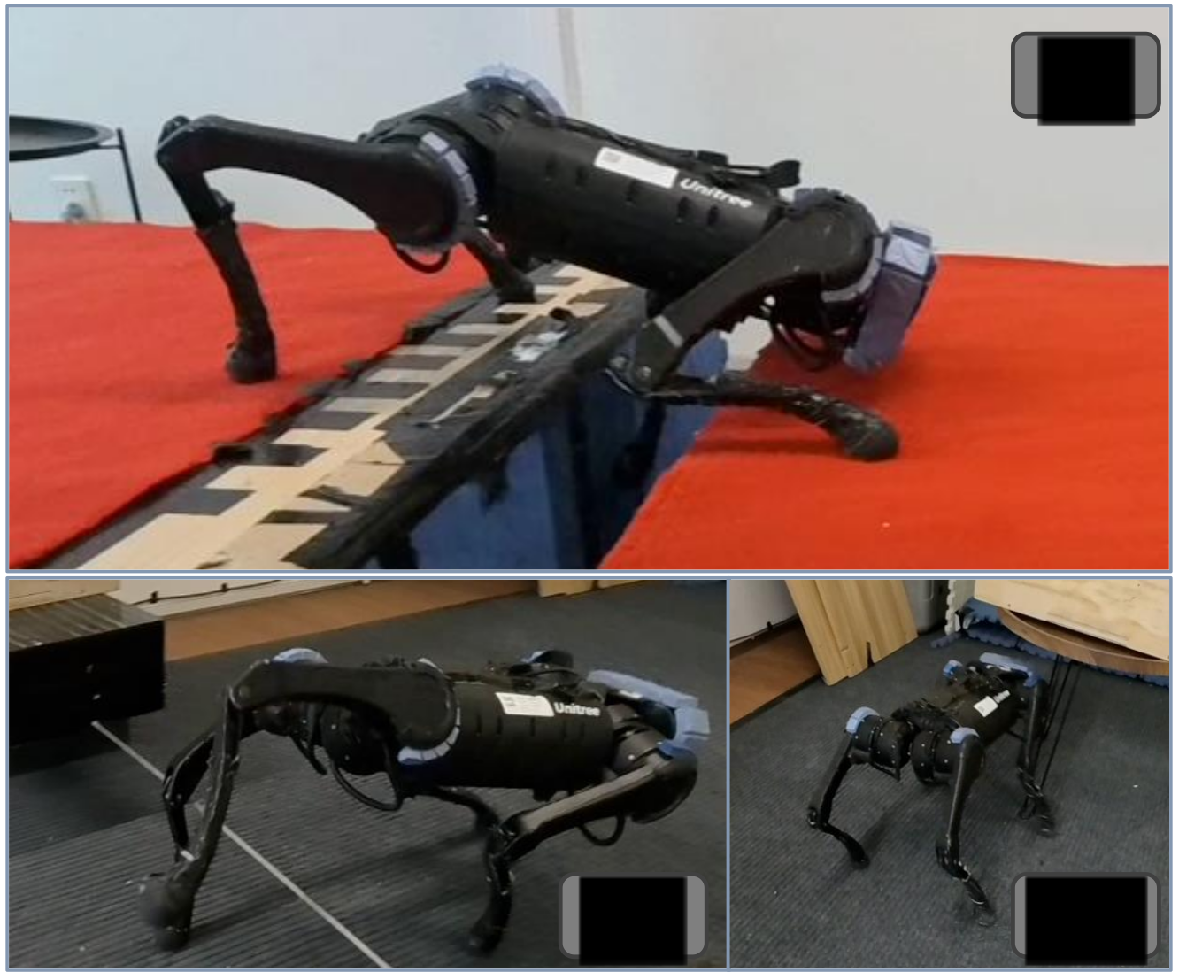
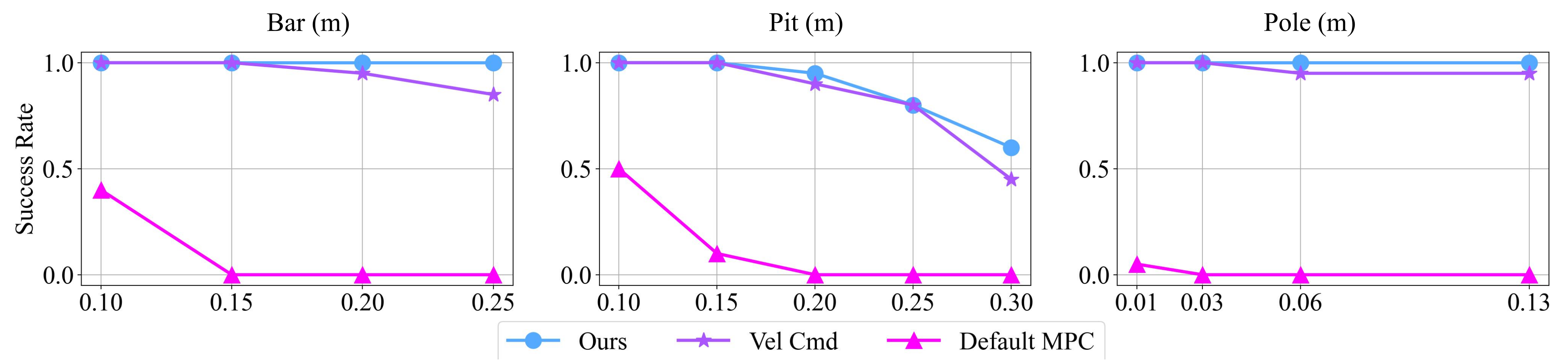
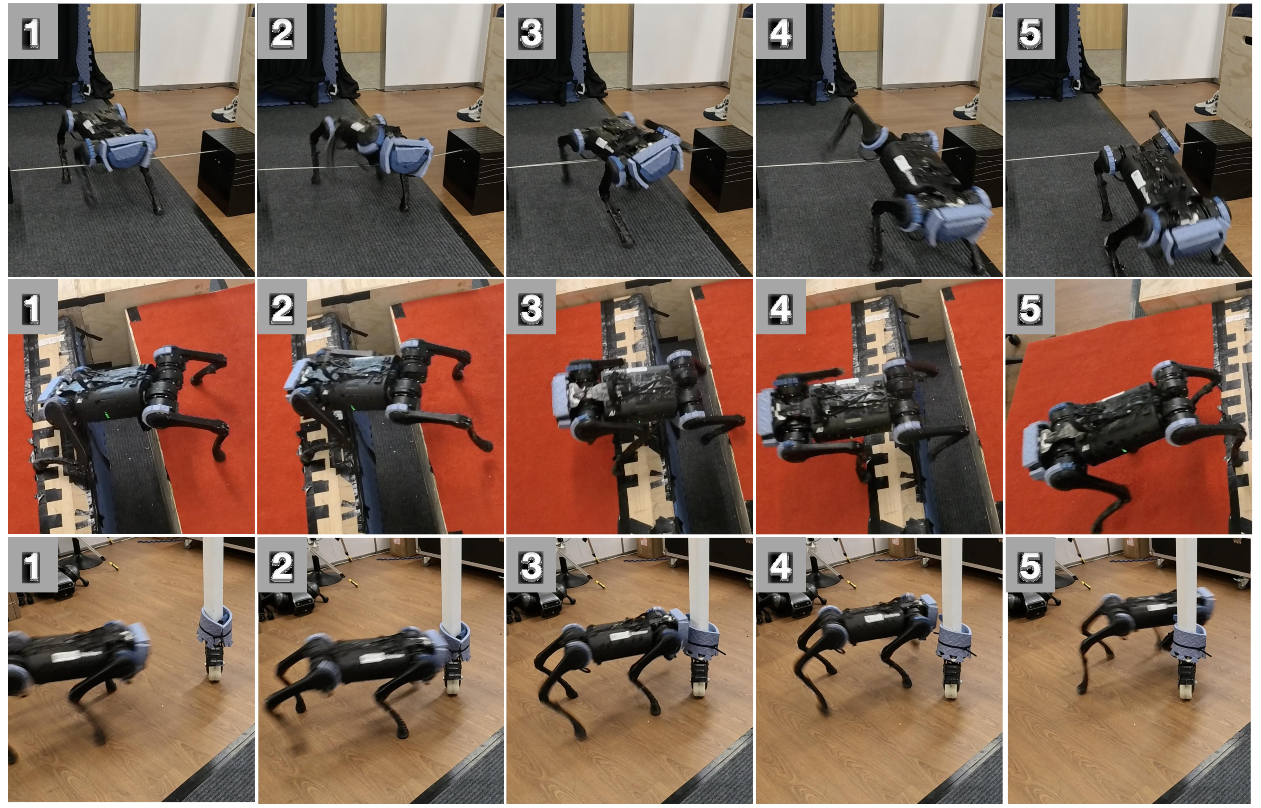
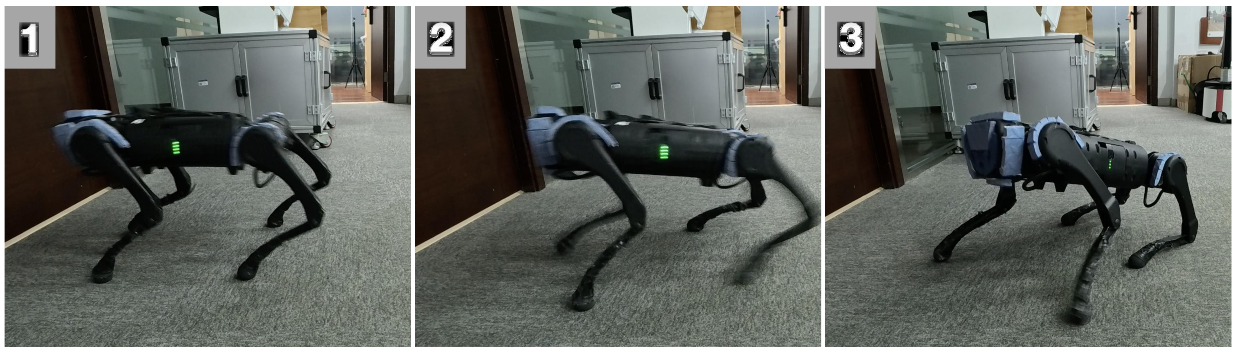
Physical behavior includes backing and lifting legs over bars, redistributing support or kicking free from pits, and sidestepping poles. Each plotted setting uses twenty repeated trials. Figure 6 compares the proposed method, a forward-velocity variant, and the default MPC controller; the proposed method performs best overall, while the velocity variant is much closer than on the long simulated courses.
Performance declines on the largest tested bar and pit settings. Figure 7 retains successful sequences, and Figure 9 retains a failure of the Boolean-contact policy after stopping and reversing on flat ground. The authors interpret that failure as a simulation-to-real mismatch in a sparse contact representation; the continuous-force encoder reduces the observed problem, without establishing that transfer errors disappear.
IV-E Additional Experiments
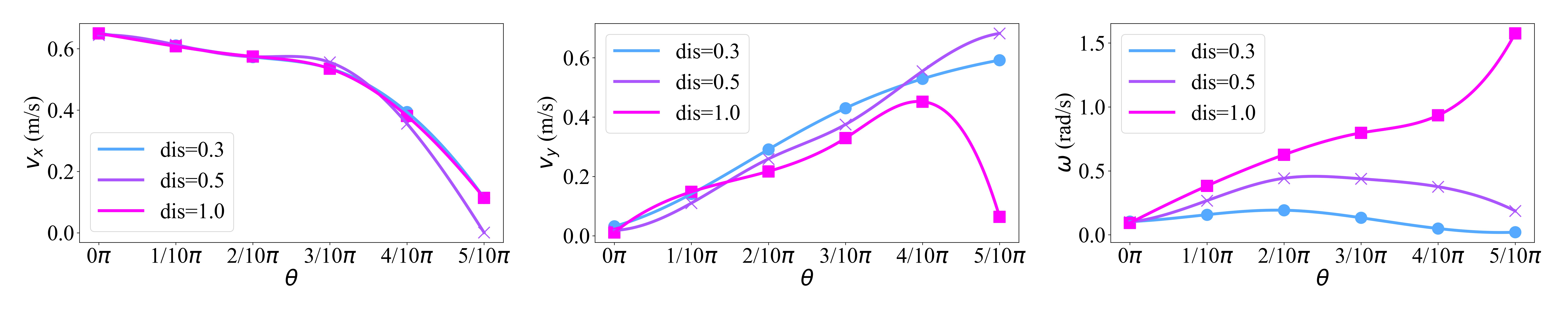
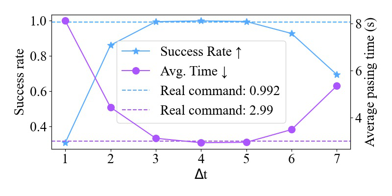
Simulation sweeps show that a constant remaining-time command of about three to five seconds works best for crossing one 0.2 m bar. Extreme values degrade performance. Sweeping goal distance and direction changes translation and turning, but the resulting speed magnitude remains constrained by the reward design.
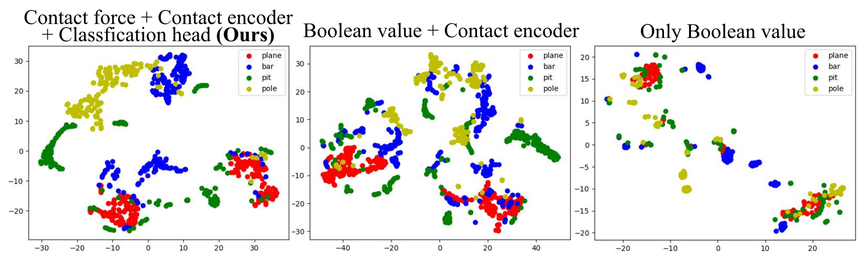
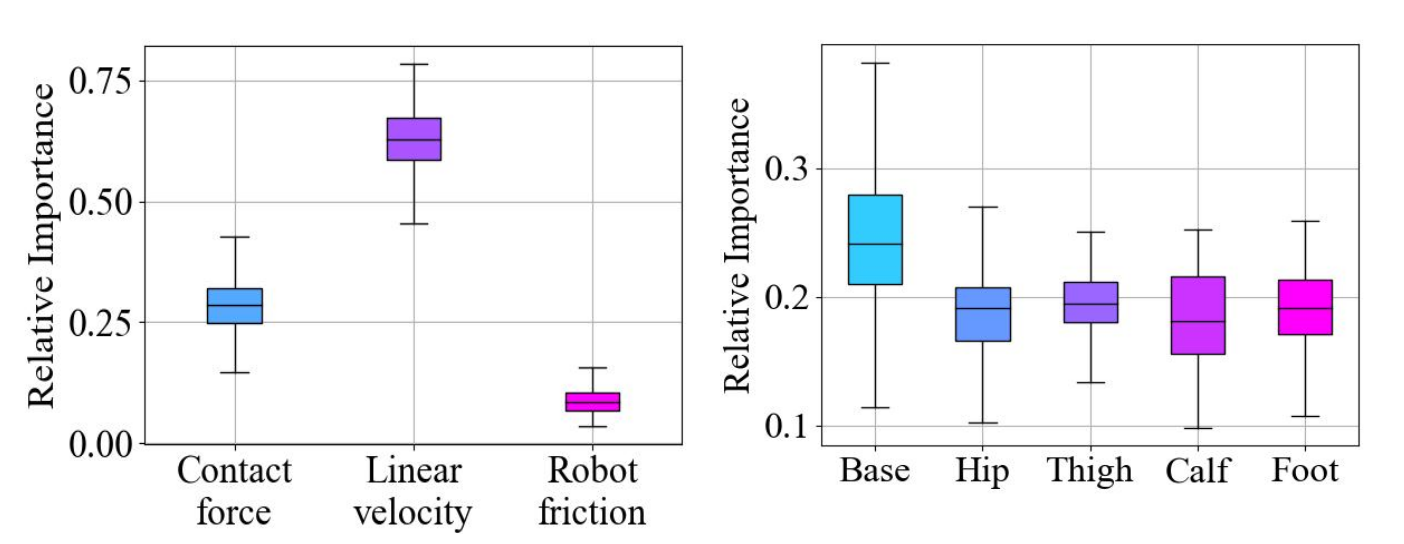
t-SNE plots make the continuous-force/classification representation look more separated and continuous than the Boolean variants. They are qualitative visualizations, not an independent test of contact-estimation accuracy. A normalized Jacobian analysis assigns roughly one quarter of grouped input sensitivity to contact information and finds the base link largest within the contact group. Sensitivity depends on input scaling and is not a causal ablation.
V CONCLUSION
The paper demonstrates contact-informed recovery over several small traps with a proprioceptive policy and a simple teleoperation interface. Practical limits include reacting only after contact, limited control of speed magnitude, training’s emphasis on forward-facing crossings, and difficulty with highly deformable obstacles such as rubber bands. Velocity-control changes and real-world finetuning are proposed future work.
APPENDIX
Appendices A–G provide reward formulas, recurrent network sizes, randomized dynamics and observation noise, terrain curriculum, optimization settings, sensitivity equations, and physical/low-light demonstrations.
| Type | Item | Formula | Weight |
| Task | Get goal | 5.0 | |
| Heading | |||
| Finish vel | -1.0 | ||
| Finish pos | -1.0 | ||
| Alive | 1 | ||
| Regularization | Stall | ||
| Vel limit | |||
| Joint vel | |||
| Joint acc | |||
| Ang vel stability | |||
| Feet in air | |||
| Balance | |||
| Style | AMP | 0.1 |
V-A Reward Functions
Table III specifies the full weighted reward. Stall and finish terms discourage unwanted immobility or motion; joint and angular-velocity terms regularize smoothness; air-time and balance terms shape gait. The heading formula differs slightly from Equation 2 by omitting the numerator’s epsilon, and both printed versions are retained.
The style reference contains 19-dimensional state transitions generated by an MPC controller: joint positions, base height, linear velocity, and angular velocity. Two hundred velocity commands run for two seconds each. A least-squares discriminator with a gradient penalty distinguishes reference from policy transitions, and its score yields Equation 12’s style reward.
Equations 12
| (12) |
V-B Network Architectures
Actor and critic are LSTMs with hidden layers [512, 256]. The estimator is an LSTM with [256, 256], followed by a [256, 256] latent MLP. The contact encoder uses [32, 16]. Table IV retains each network’s input and output; privileged critic/contact inputs are training signals rather than deployed sensors.
V-C Dynamic Randomization
Randomization covers base mass, center-of-mass offsets, friction, initial joints and velocity, motor strength, and proprioception latency. Table V prints a base-mass range of 0–3 kg without clearly identifying whether it is an offset, and a latency range of 0.2–0.4 seconds; these values are retained without reinterpretation.
Table VI adds observation noise to velocity, gravity, and joint signals. The paper attributes improved transfer to these variations, but does not isolate each randomization source’s effect.
| Parameters | Range | Unit |
|---|---|---|
| Base mass | [0, 3] | |
| Mass position of X axis | [-0.2, 0.2] | |
| Mass position of Y axis | [-0.1, 0.1] | |
| Mass position of Z axis | [-0.05, 0.05] | |
| Friction | [0, 2] | - |
| Initial joint positions | [0.5, 1.5]nominal value | |
| Initial base velocity | [-1.0, 1.0] (all directions) | |
| Motor strength | [0.9, 1.1]nominal value | - |
| Proprioception latency | [0.2, 0.4] |
| Observation | Gaussian Noise Amplitude | Unit |
|---|---|---|
| Linear velocity | 0.05 | |
| Angular velocity | 0.2 | |
| Gravity | 0.05 | |
| Joint position | 0.01 | |
| Joint velocity | 1.5 |
V-D Trap Terrain Setting in Simulation
A 10×10 terrain grid allocates three columns to bars, two to pits, three to poles, and two to planes, with ten difficulty levels. Circular bars and pits prevent bypassing the obstacle. Bar heights grow from 0.05–0.25 m, pit widths from 0.05–0.30 m, and pole counts from ten to sixty; bar/pole widths vary from 0.025–0.10 m. Perlin-noise amplitudes range from 0.05–0.15 m.
V-E Training Hyperparameters
Table VII retains PPO settings, including learning rate 0.001, clipping 0.2, discount 0.99, GAE parameter 0.95, and four minibatches. Its twenty-four rollout steps differ from the main text’s fifty. Contact forces are clipped to 0–100 N before the reported normalization. Table VIII gives t-SNE initialization, perplexity thirty, and learning rate two hundred.
| Hyperparameter | Value |
|---|---|
| clip min std | 0.05 |
| clip param | 0.2 |
| desired kl | 0.01 |
| entropy coef | 0.01 |
| gamma | 0.99 |
| lam | 0.95 |
| learning rate | 0.001 |
| max grad norm | 1 |
| num mini batch | 4 |
| num steps per env | 24 |
| Hyperparameter | Value |
|---|---|
| init | ‘random’ |
| perplexity | 30 |
| learning rate | 200 |
V-F Importance Analysis
The analysis differentiates actions with respect to inputs, takes absolute derivatives, scales each input by its specified range, sums across actions, then averages and normalizes by input group. Equations 13–18 retain the calculation. The final denominator uses an N-indexed sum although the text defines k comparison groups; the original expression remains unchanged. These normalized derivatives measure local model sensitivity under the chosen scaling.
Equations 13–18
| (13) |
| (14) |
| (15) |
| (16) |
| (17) |
| (18) |
V-G Real-world Experiment Settings and Additional Results
Physical traps include 6 mm and 20 mm bars, 8 mm table-leg poles, larger poles/sticks, and gaps between 40 mm-high wooden boxes. The photographed objects and all low-light crossing sequences are retained. The demonstration dimensions differ slightly from Figure 6’s rounded plotted pole-width range.
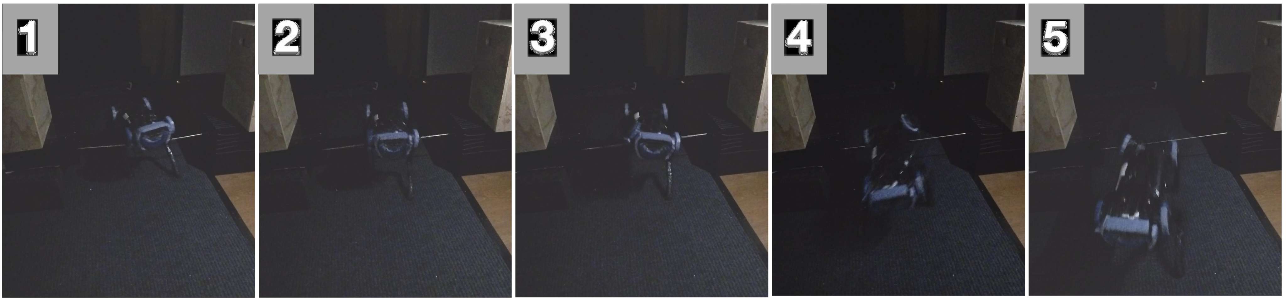
The robot also crosses bars, pits, and poles in low light without visual input. These sequences illustrate the sensor choice’s usefulness in darkness; the appendix does not report a separate low-light trial count or aggregate success rate.